Gromov-Wasserstein Distance based Object Matching: Asymptotic Inference

Christoph Alexander Weitkamp Note: Institute for Mathematical Stochastics, University of Göttingen, Goldschmidtstraße 7, 37077 Göttingen Katharina Proksch Note: Faculty of Electrical Engineering, Mathematics & Computer Science, University of Twente, Hallenweg 19, 7522NH Enschede Carla Tameling ^†^†footnotemark: Axel Munk ^†^†footnotemark: Note: Max Planck Institute for Biophysical Chemistry, Am Faßberg 11, 37077 Göttingen

Abstract

In this paper, we aim to provide a statistical theory for object matching based on the Gromov-Wasserstein distance. To this end, we model general objects as metric measure spaces. Based on this, we propose a simple and efficiently computable asymptotic statistical test for pose invariant object discrimination. This is based on an empirical version of a $\beta$ -trimmed lower bound of the Gromov-Wasserstein distance. We derive for $\beta\in[0,1/2)$ distributional limits of this test statistic. To this end, we introduce a novel $U$ -type process indexed in $\beta$ and show its weak convergence. Finally, the theory developed is investigated in Monte Carlo simulations and applied to structural protein comparisons.

Keywords Gromov-Wasserstein distance, metric measures spaces, U-processes, distributional limits, protein matching

MSC 2010 subject classification Primary: 62E20, 62G20, 65C60 Secondary: 60E05

1 Introduction

Over the last decades, the acquisition of geometrically complex data in various fields of application has increased drastically. For the digital organization and analysis of such data it is important to have meaningful notions of similarity between datasets as well as between shapes. This most certainly holds true for the area of 3-D object matching, which has many relevant applications, for example in computer vision (Viola and Jones 2001; Torralba et al. 2003), mechanical engineering (Au and Yuen 1999; El-Mehalawi and Miller 2003) or molecular biology Nussinov and Wolfson 1991; Sandak et al. 1995; Krissinel and Henrick 2004. In most of these applications, an important challenge is to distinguish between shapes while regarding identical objects in different spatial orientations as equal. A prominent example is the comparison of 3-D protein structures, which is important for understanding structural, functional and evolutionary relationships among proteins Kolodny et al. 2005; Srivastava et al. 2016. Most known protein structures are published as coordinate files, where for every atom a 3-D coordinate is estimated based on an indirect observation of the protein’s electron density (see Rhodes 2010 for further details), and stored e.g. in the protein database PDB Berman et al. 2000. These coordinate files lack any kind of orientation and any meaningful comparison has to take this into account. Figure 1 (created with PyMOL Schrödinger, LLC 2015) shows two cartoon representations of the backbone of the protein structure 5D0U in two different poses. These two representations obtained from the same coordinate file highlight the difficulty to identify them from noisy measurements.

Refer to caption — Figure 1: Illustration of the proteins to be compared: Cartoon representation of the DEAH-box RNA-helicase Prp43 from chaetomium thermophilum bound to ADP (PDB ID: 5D0U Tauchert et al. 2016) in two different poses. The DEAH-box helicase Prp43 unwinds double stranded RNA and rearranges RNA/protein complexes. It has essential roles in pre-mRNA splicing and ribosome biogenesis Arenas and Abelson 1997; Lebaron et al. 2005.

Consequently, many approaches to pose invariant shape matching, classification and recognition have been suggested and studied in the literature. The majority of these methods computes and compares certain invariants or signatures in order to decide whether the considered objects are equal up to a previously defined notion of invariance. In the literature, these methods are often called feature (or signature) based methods, see Cárdenas et al. 2005 for a comprehensive survey. Some examples for features are the shape distributions (Osada et al. 2002), that are connected to the distributions of lengths, areas and volumes of an object, the shape contexts (Belongie et al. 2002), that rely in a sense on a local distribution of inter-point distances of the considered object, and reduced size functions (d’Amico et al. 2008), which count the connected components of certain lower level sets.
As noted by Mémoli 2007; Mémoli 2011, several signatures describe different aspects of a metric between objects. In these and subsequent papers, the author develops a unifying view point by representing an object as metric measure space $\left(\mathcal{X},d_{\mathcal{X}},\mu_{\mathcal{X}}\right)$ , where $\left(\mathcal{X},d_{\mathcal{X}}\right)$ is a compact metric space and $\mu_{\mathcal{X}}$ denotes a Borel probability measure on $\mathcal{X}$ . The additional probability measure, whose support is assumed to be $\mathcal{X}$ , can be thought of as signaling the importance of different regions of the modeled object. Based on the original work of Gromov 1999, Mémoli 2011 introduced the Gromov-Wasserstein distance of order $p\in[1,\infty)$ between two (compact) metric measure spaces $\left(\mathcal{X},d_{\mathcal{X}},\mu_{\mathcal{X}}\right)$ and $\left(\mathcal{Y},d_{\mathcal{Y}},\mu_{\mathcal{Y}}\right)$ which will be fundamental to this paper. We allow ourselves to rename it to Gromov-Kantorovich distance to give credit to Kantorovich’s initial work Kantorovich 1942 underlying this concept (see Vershik 2013). It is defined as

{\mathcal{GK}_{p}}(\mathcal{X},\mathcal{Y})=\inf_{\pi\in\mathcal{M}(\mu_{\mathcal{X}},\mu_{\mathcal{Y}})}J_{p}(\pi),

(1)

where

\displaystyle J_{p}(\pi)\coloneqq

\displaystyle\frac{1}{2}\left(\int_{\mathcal{X}\times\mathcal{Y}}\int_{\mathcal{X}\times\mathcal{Y}}\!\left|d_{\mathcal{X}}(x,x^{\prime})-d_{\mathcal{Y}}(y,y^{\prime})\right|^{p}\,\pi(dx\times dy)\,\pi(dx^{\prime}\times dy^{\prime})\right)^{\frac{1}{p}}.

Here, $\mathcal{M}(\mu_{\mathcal{X}},\mu_{\mathcal{Y}})$ stands for the set of all couplings of $\mu_{\mathcal{X}}$ and $\mu_{\mathcal{Y}}$ , i.e., the set of all measures $\pi$ on the product space $\mathcal{X}\times\mathcal{Y}$ such that

\pi\left(A\times\mathcal{Y}\right)=\mu_{\mathcal{X}}\left(A\right)~\mathrm{and}~\pi\left(\mathcal{X}\times B\right)=\mu_{\mathcal{Y}}\left(B\right)

for all measurable sets $A\subset\mathcal{X}$ and $B\subset\mathcal{Y}$ . In Section 5 of Mémoli 2011 it is ensured that the Gromov-Kantorovich distance ${\mathcal{GK}_{p}}$ is suitable for pose invariant object matching by proving that it is a metric on the collection of all isomorphism classes of metric measure spaces.¹¹ 1 Two metric measure spaces $\left(\mathcal{X},d_{\mathcal{X}},\mu_{\mathcal{X}}\right)$ and $\left(\mathcal{Y},d_{\mathcal{Y}},\mu_{\mathcal{Y}}\right)$ are isomorphic (denoted as $\left(\mathcal{X},d_{\mathcal{X}},\mu_{\mathcal{X}}\right)\cong\left(\mathcal{Y},d_{\mathcal{Y}},\mu_{\mathcal{Y}}\right)$ ) if and only if there exists an isometry $\phi:\mathcal{X}\to\mathcal{Y}$ such that $\phi\#\mu_{\mathcal{X}}=\mu_{\mathcal{Y}}$ . Here, $\phi\#\mu_{\mathcal{X}}$ denotes the pushforward measure. Hence, objects are considered to be the same if they can be transformed into each other without changing the distances between their points and such that the corresponding measures are preserved. For example, if the distance is Euclidean, this leads to identifying objects up to translations, rotations and reflections Lomont 2014.

The definition of the Gromov-Kantorovich distance extends the Gromov-Hausdorff distance, which is a metric between compact metric spaces Mémoli and Sapiro 2004; Mémoli and Sapiro 2005; Mémoli 2007. The additional measure structure of metric measure spaces allows to replace the Hausdorff distance component in the definition of the Gromov-Hausdorff distance by a relaxed notion of proximity, namely the Kantorovich distance (Kantorovich 1942). This distance is fundamental to a variety of mathematical developments and is also known in different communities as the Wasserstein distance Vaserstein 1969, Kantorovich-Rubinstein distance (Kantorovich and Rubinstein 1958), Mallows distance (Mallows 1972) or as the Earth Mover’s distance (Rubner et al. 2000). The Kantorovich distance of order $p$ ( $p\geq 1$ ) between two probability measures $\mu_{\mathcal{X}}$ and $\nu_{\mathcal{X}}$ on the compact metric space $\left(\mathcal{X},d_{\mathcal{X}}\right)$ is defined as

{\mathcal{K}_{p}}(\mu_{\mathcal{X}},\nu_{\mathcal{X}})=\left\{\inf_{\pi\in\mathcal{M}(\mu_{\mathcal{X}},\nu_{\mathcal{X}})}\int_{\mathcal{X}\times\mathcal{X}}\!\,d^{p}_{\mathcal{X}}(x,y)\,d\pi(x,y)\right\}^{\frac{1}{p}},

(2)

where $\mathcal{M}(\mu_{\mathcal{X}},\nu_{\mathcal{X}})$ denotes the set of all couplings of $\mu_{\mathcal{X}}$ and $\nu_{\mathcal{X}}$ . Let $\mathcal{P}(\mathcal{X})$ be the space of all probability measures on $\mathcal{X}$ . Then, as compact metric spaces are in particular Polish, the Kantorovich distance defines a metric on

\mathcal{P}_{p}\left(\mathcal{X}\right)=\bigg\{\mu\in\mathcal{P}(\mathcal{X})~\bigg|~\int_{\mathcal{X}}d^{p}_{\mathcal{X}}(x_{0},x)\,d\mu(x)<\infty,~x_{0}\in\mathcal{X}~\mathrm{arbitrary}\bigg\}

and it metrizes weak convergence together with convergence of moments of order $p$ (Villani 2008).

Due to its measure preserving metric invariance, the Gromov-Kantorovich distance is conceptually well suited for pose invariant object discrimination. Heuristically speaking, the Gromov-Kantorovich point of view suggests to regard a data cloud as a metric measure space by itself, which takes into account its internal metric structure (encoded in its pairwise distances), and provides a transportation between metric spaces without loss of mass. In particular, it does not rely on the embedding in an external space. For the above described protein comparison problem, the coordinate system in which the atoms are represented does not matter. Hence, the Gromov-Kantorovich distance is only influenced by the internal relations between the backbone atoms - which matches the physical understanding of structural similarity in this context. However, the practical usage of the Gromov-Kantorovich approach is severely hindered by its computational complexity: For two finite metric measure spaces $\mathcal{X}=\left\{x_{1},\dots,x_{n}\right\}$ and $\mathcal{Y}=\left\{y_{1},\dots,y_{m}\right\}$ with metrics $d_{\mathcal{X}}$ and $d_{\mathcal{Y}}$ and probability measures $\mu_{\mathcal{X}}$ and $\mu_{\mathcal{Y}}$ , respectively, the computation of ${\mathcal{GK}_{p}}\left(\mathcal{X},\mathcal{Y}\right)$ boils down to solving a (non-convex) quadratic program (Mémoli 2011, Sec. 7). This is in general NP-hard (Pardalos and Vavasis 1991). To circumvent the precise determination of the Gromov-Kantorovich distance, it has been suggested to approximate it via gradient descent Mémoli 2011 or to relax the corresponding optimization problem. For example, Solomon et al. 2016 proposed the entropic Gromov-Kantorovich distance, which has been applied to find correspondences between word embedding spaces, an important task for machine translation Alvarez-Melis and Jaakkola 2018. In this paper, we take a different route and investigate the potential of a lower bound for $\mathcal{GK}_{p}$ , which is on the one hand extremely simple to compute in $O(n^{2})$ elementary operations and on the other hand statistically accessible and useful for inference tasks, in particular for object discrimination when the data are randomly sampled or the data set is massive and subsampling becomes necessary. As this bound quantifies the optimal transport distance between the distributions of pairwise distances (see Section 1.1), we believe that our analysis is of quite general statistical interest beyond the described scenario.

1.1 The Proposed Approach

Given two metric measure spaces, denoted as $\left(\mathcal{X},d_{\mathcal{X}},\mu_{\mathcal{X}}\right)$ and $\left(\mathcal{Y},d_{\mathcal{Y}},\mu_{\mathcal{Y}}\right)$ , we aim to construct an (asymptotic) test for the hypothesis that these spaces are isomorphic, viz.

\displaystyle H_{0}:~\left(\mathcal{X},d_{\mathcal{X}},\mu_{\mathcal{X}}\right)\cong\left(\mathcal{Y},d_{\mathcal{Y}},\mu_{\mathcal{Y}}\right),

(3)

against the alternative

\displaystyle H_{1}:~\left(\mathcal{X},d_{\mathcal{X}},\mu_{\mathcal{X}}\right)\ncong\left(\mathcal{Y},d_{\mathcal{Y}},\mu_{\mathcal{Y}}\right).

(4)

This test will be based on an efficiently computable empirical version of a lower bound of the Gromov-Kantorovich distance.

Let $\mu^{U}$ be the probability measure of the random variable $d_{\mathcal{X}}(X,X^{\prime})$ , where $X,X^{\prime}\overset{i.i.d.}{\sim}\mu_{\mathcal{X}}$ , and let $\mu^{V}$ be the one of $d_{\mathcal{Y}}(Y,Y^{\prime})$ , with $Y,Y^{\prime}\overset{i.i.d.}{\sim}\mu_{\mathcal{Y}}$ . Then, we call $\mu^{U}$ and $\mu^{V}$ the distribution of the (pairwise) distances of $\left(\mathcal{X},d_{\mathcal{X}},\mu_{\mathcal{X}}\right)$ and $\left(\mathcal{Y},d_{\mathcal{Y}},\mu_{\mathcal{Y}}\right)$ , respectively. Fundamental to our approach is the fact that the Gromov-Kantorovich distance between two metric measure spaces $\left(\mathcal{X},d_{\mathcal{X}},\mu_{\mathcal{X}}\right)$ and $\left(\mathcal{Y},d_{\mathcal{Y}},\mu_{\mathcal{Y}}\right)$ of order $p\in[1,\infty)$ is lower bounded by

{\mathcal{GK}_{p}}(\mathcal{X},\mathcal{Y})\geq\frac{1}{2}\!\left(DoD_{p}\left(\mathcal{X},\mathcal{Y}\right)\right)^{\frac{1}{p}}\coloneqq\frac{1}{2}\left(\int_{0}^{1}\!\left|U^{-1}(t)-V^{-1}(t)\right|^{p}dt\right)^{\frac{1}{p}},

(5)

where $U^{-1}$ and $V^{-1}$ are the quantile functions of $\mu^{U}$ and $\mu^{V}$ , respectively Mémoli 2011. If the right hand side of (5) is positive, so is ${\mathcal{GK}_{p}}$ and it is thus possible to base a statistical test for $H_{0}$ on an empirical version of this quantity. Furthermore, the above lower bound possesses several theoretical and practical features that make it worthy of study:

1.) Reformulating (5) yields that the Gromov-Kantorovich distance between two metric measure spaces is lower bounded by the Kantorovich distance of the respective distributions of distances (one dimensional quantities), i.e.,

DoD_{p}(\mathcal{X},\mathcal{Y})=\mathcal{K}_{p}^{p}\left(\mu^{U},\mu^{V}\right)=\inf_{\pi\in\mathcal{M}\left(\mu^{U},\mu^{V}\right)}\int_{\mathbb{R}\times\mathbb{R}}\!\,|x-y|^{p}\,d\pi(x,y).

Interestingly, there is another reformulation of $DoD_{p}$ in terms of an optimal transport problem between the product measures $\mu_{\mathcal{X}}\otimes\mu_{\mathcal{X}}$ and $\mu_{\mathcal{Y}}\otimes\mu_{\mathcal{Y}}$ . It is shown in (Chowdhury and Mémoli 2019, Thm. 24) that

DoD_{p}\left(\mathcal{X},\mathcal{Y}\right)\!=\!\inf_{\pi\in\widetilde{\mathcal{M}}}\,\int_{\mathcal{X}\times\mathcal{X}\times\mathcal{Y}\times\mathcal{Y}}\left|d_{\mathcal{X}}(x,x^{\prime})-d_{\mathcal{Y}}(y,y^{\prime})\right|^{p}d\pi(x,x^{\prime}y,y^{\prime}),

(6)

where $\widetilde{\mathcal{M}}\coloneqq\mathcal{M}(\mu_{\mathcal{X}}\otimes\mu_{\mathcal{X}},\mu_{\mathcal{Y}}\otimes\mu_{\mathcal{Y}})$ . This representation emphasizes the relation between $DoD_{p}$ and the Gromov-Kantorovich distance defined in (1), as clearly $\pi\otimes\pi\in\widetilde{\mathcal{M}}$ for all $\pi\in\mathcal{M}(\mu_{\mathcal{X}},\mu_{\mathcal{Y}})$ .

2.) Although it is known that the distribution of distances does not uniquely characterize a metric measure space Mémoli 2011, it was proposed as a feature itself for feature based object matching and was shown to work well in practice in various examples Osada et al. 2002; Brinkman and Olver 2012; Berrendero et al. 2016; Gellert et al. 2019. In fact, Gellert et al. 2019 applied several lower bounds of the Gromov-Kantorovich distance stated in Mémoli 2011 for the comparison of the isosurfaces of various proteins. The authors empirically found that $DoD_{p}$ defined in (5) has high discriminative abilities for this task.

3.) Generally, $DoD_{p}$ is a simple and natural measure to compare distance matrices. Such distance matrices underlie many methods of data analysis, e.g. various multidimensional scaling techniques (see Dokmanic et al. 2015).

4.) The representation (5) admits an empirical version which is computable in effectively $O\left((m\vee n)^{2}\right)$ operations, if the computation of one distance is considered as $O(1)$ . To this end, let $X_{1},\dots,X_{n}\overset{i.i.d.}{\sim}\mu_{\mathcal{X}}$ and $Y_{1},\dots,Y_{m}\overset{i.i.d.}{\sim}\mu_{\mathcal{Y}}$ be two independent samples and let $\mathcal{X}_{n}=\left\{X_{1},\dots,X_{n}\right\}$ and $\mathcal{Y}_{m}=\left\{Y_{1},\dots,Y_{m}\right\}$ . The sample analog to (5) is to be defined with respect to the empirical measures and we obtain as empirical counterpart to (5) the DoD-statistic as

\widehat{{DoD}}_{p}=\widehat{{DoD}}_{p}\left(\mathcal{X}_{n},\mathcal{Y}_{m}\right)\coloneqq\int_{0}^{1}\!\left|U^{-1}_{n}(t)-V^{-1}_{m}(t)\right|^{p}\,dt,

(7)

where, for $t\in\mathbb{R}$ , $U_{n}$ is defined as the empirical c.d.f. of all pairwise distances of the sample $\mathcal{X}_{n}$ ,

U_{n}(t)\coloneqq\frac{2}{n(n-1)}\sum_{1\leq i<j\leq n}\mathds{1}_{\left\{d_{\mathcal{X}}(X_{i},X_{j})\leq t\right\}}.

(8)

Analogously, we define for the sample $\mathcal{Y}_{n}$

V_{m}(t)\coloneqq\frac{2}{m(m-1)}\sum_{1\leq k<l\leq m}\mathds{1}_{\left\{d_{\mathcal{Y}}(Y_{k},Y_{l})\leq t\right\}}.

(9)

Besides, $U^{-1}_{n}$ and $V^{-1}_{m}$ denote the corresponding empirical quantile functions. We stress that the evaluation of $\widehat{{DoD}}_{p}$ boils down to the calculation of a sum and no formal integration is required. For $n=m$ it holds

\widehat{{DoD}}_{p}=\frac{2}{n(n-1)}\sum_{i=1}^{n(n-1)/2}\left|d^{\mathcal{X}}_{(i)}-d^{\mathcal{Y}}_{(i)}\right|^{p},

where $d^{\mathcal{X}}_{(i)}$ denotes the $i$ -th order statistic of the sample $\left\{d_{\mathcal{X}}(X_{i},X_{j})\right\}_{1\leq i<j\leq n}$ and $d^{\mathcal{Y}}_{(i)}$ is defined analogously. For $n\neq m$ we obtain that

\widehat{{DoD}}_{p}=\sum_{i=1}^{\frac{n(n-1)}{2}}\sum_{j=1}^{\frac{m(m-1)}{2}}\lambda_{ij}\left|d^{\mathcal{X}}_{(i)}-d^{\mathcal{Y}}_{(j)}\right|^{p},

where

\lambda_{ij}=\left(\frac{i}{n}\wedge\frac{j}{m}-\frac{i-1}{n}\vee\frac{j-1}{m}\right)\mathds{1}_{\left\{{i}{m}\wedge{j}{n}>{(i-1)}{m}\vee{(j-1)}{n}\right\}}.

Here, and in the following, $a\wedge b$ denotes the minimum and $a\vee b$ the maximum of two real numbers $a$ and $b$ .

1.2 Main Results

The main contributions of the paper are various upper bounds and distributional limits for the statistic defined in (7) (as well as trimmed variants). Based on these, we design an asymptotic test that compares two distributions of distances and thus obtain an asymptotic test for the hypothesis $H_{0}$ defined in (3). In the course of this, we focus, for ease of notation, on the case $p=2$ , i.e., we derive for $\beta\in[0,1/2)$ the limit behavior of the statistic

\widehat{DoD}_{(\beta)}\coloneqq\int_{\beta}^{1-\beta}\!\left(U_{n}^{-1}(t)-V_{m}^{-1}(t)\right)^{2}\,dt

under the hypothesis (3) as well as under the alternative in (4). The introduced trimming parameter $\beta$ can be used to robustify the proposed method Czado and Munk 1998; Alvarez-Esteban et al. 2008. Most of our findings can easily be transferred to the case of $p\in[1,\infty)$ , which is readdressed in Section 2.3. Next, we briefly summarize the setting in which we are working and introduce the conditions required.

Setting 1.1.

Let $\left(\mathcal{X},d_{\mathcal{X}},\mu_{\mathcal{X}}\right)$ and $\left(\mathcal{Y},d_{\mathcal{Y}},\mu_{\mathcal{Y}}\right)$ be two metric measure spaces and let $\mu^{U}$ and $\mu^{V}$ denote the distributions of (pairwise) distances of the spaces $\left(\mathcal{X},d_{\mathcal{X}},\mu_{\mathcal{X}}\right)$ and $\left(\mathcal{Y},d_{\mathcal{Y}},\mu_{\mathcal{Y}}\right)$ , respectively. Let $U$ denote the c.d.f. of $\mu^{U}$ , assume that $U$ is differentiable with derivative $u$ and let $U^{-1}$ be the quantile function of $U$ . Let $V$ , $V^{-1}$ and $v$ be defined analogously. Further, let the samples $X_{1},\dots,X_{n}\overset{i.i.d.}{\sim}\mu_{\mathcal{X}}$ and $Y_{1},\dots,Y_{m}\overset{i.i.d.}{\sim}\mu_{\mathcal{Y}}$ be independent of each other and let $U^{-1}_{n}$ and $V^{-1}_{m}$ denote the empirical quantile functions of $U_{n}$ defined in (8) and $V_{m}$ defined in (9).

Since the statistic $\widehat{DoD}_{(\beta)}$ is based on empirical quantile functions, or more precisely empirical $U$ -quantile functions, we have to ensure that the corresponding $U$ -distribution functions are well-behaved. In the course of this, we distinguish the cases $\beta\in(0,1/2)$ and $\beta=0$ . The subsequent condition guarantees that the inversion functional $\phi_{inv}:F\mapsto F^{-1}$ is Hadamard differentiable as a map from the set of restricted distribution functions into the space of all bounded functions on $[\beta,1-\beta]$ , in the following denoted as $\ell^{\infty}[\beta,1-\beta]$ .

Condition 1.2.

Let $\beta\in(0,1/2)$ and let $U$ be continuously differentiable on an interval

[C_{1},C_{2}]=[U^{-1}(\beta)-\epsilon,U^{-1}(1-\beta)+\epsilon]

for some $\epsilon>0$ with strictly positive derivative $u$ and let the analogue assumption hold for $V$ and its derivative $v$ .

When the densities of $\mu^{U}$ and $\mu^{V}$ vanish at the boundaries of their support, which commonly happens (see 2.1), we can no longer rely on Hadamard differentiability to derive the limit distribution of $\widehat{DoD}_{(\beta)}$ under $H_{0}$ for $\beta=0$ . In order to deal with this case we require stronger assumptions. The following ones resemble those of Mason 1984.

Condition 1.3.

Let $U$ be continuously differentiable on its support. Further, assume there exist constants $-1<\gamma_{1},\gamma_{2}<\infty$ and $c_{U}>0$ such that

\left|(U^{-1})^{\prime}(t)\right|\leq c_{U}t^{\gamma_{1}}(1-t)^{\gamma_{2}}

for $t\in(0,1)$ and let the analogue assumptions hold for $V$ and $(V^{-1})^{\prime}$ .

Both, 1.2 and 1.3 are comprehensively discussed in Section 2.1 and various illustrative examples are given there.

With the main assumptions stated we can now specify the results derived under the hypothesis $H_{0}$ and afterwards those under the alternative $H_{1}$ . Under $H_{0}$ we have that the distributions of distances of the considered metric measure spaces, $\mu^{U}$ and $\mu^{V}$ , are equal, i.e., $U(t)=V(t)$ for $t\in\mathbb{R}$ . Given 1.2 we find that for $\beta\in(0,1/2)$ (resp. given 1.3 for $\beta=0$ ) and $n,m\to\infty$

\displaystyle\frac{nm}{n+m}\widehat{DoD}_{(\beta)}\rightsquigarrow\Xi=\Xi(\beta)\coloneqq\int_{\beta}^{1-\beta}\!\left(\mathbb{G}(t)\right)^{2}\,dt,

(10)

where $\mathbb{G}$ is a centered Gaussian process with covariance depending on $U$ (under $H_{0}$ we have $U=V$ ) in an explicit but complicated way, see 2.4. Further, “ $\rightsquigarrow$ ” denotes weak convergence in the sense of Hoffman-Jørgensen (see van der Vaart and Wellner 1996). Additionally, we establish in Section 2 a simple concentration bound for $\widehat{DoD}_{(\beta)}$ and demonstrate that for $\beta\in(0,1/2)$ and $\alpha\in(0,1)$ the corresponding $\alpha$ -quantile of $\Xi$ , which is required for testing, can be obtained by a bootstrap scheme, see Section 3.

Next, we summarize our findings under $H_{1}$ . As we work with a lower bound, the limit behavior under the alternative is a little more complex. Under the additional assumption that

DoD_{(\beta)}\coloneqq\int_{\beta}^{1-\beta}\!\left(U^{-1}(t)-V^{-1}(t)\right)^{2}\,dt>0,

we can prove (cf. ) that given 1.2 it holds for $n,m\to\infty$ and $\beta\in(0,1/2)$ (resp. given 1.3 for $\beta=0$ ) that

\sqrt{\frac{nm}{n+m}}\left(\widehat{DoD}_{(\beta)}-DoD_{(\beta)}\right)\rightsquigarrow N(0,\sigma_{U,V,\lambda}^{2}),

(11)

where $N(0,\sigma_{U,V,\lambda}^{2})$ denotes a normal distribution with mean 0 and variance $\sigma_{U,V,\lambda}^{2}$ depending on $U$ , $V$ , $\beta$ and $\lambda=\lim_{n,m\to\infty}\frac{n}{m+n}$ .

1.3 Applications

From our theory it follows that for $\beta\in[0,1/2)$ a (robust) asymptotic level- $\alpha$ -test for $H_{0}$ against $H_{1}$ is given by rejecting $H_{0}$ in (3) if

\frac{nm}{n+m}\widehat{DoD}_{(\beta)}>\xi_{1-\alpha},

(12)

where $\xi_{1-\alpha}$ denotes the $(1-\alpha)$ -quantile of $\Xi$ . The simulations in Section 4 demonstrate that, although it is based on a lower bound of the Gromov-Kantorovich distance $\mathcal{GK}_{p}$ between the metric measure spaces, the proposed test (as well as its bootstrap version) represents a powerful method to detect deviations between metric measure spaces in the sense of (3). This has many possible applications.

Exemplarily, in Section 5, we model proteins as such metric measure spaces by assuming that the coordinate files are samples from (unknown) distributions (see Rhodes 2010) and apply the theory developed to compare the protein structures depicted in Figure 2. Our major findings can be summarized as follows:

5D0U vs 5JPT: 5D0U and 5JPT are two structures of the same protein extracted from different organisms. Consequently, their secondary structure elements can almost be aligned perfectly (see Figure 2, left). Only small parts of the structures are slightly shifted and do not overlap in the alignment. Applying (12) for this comparison generally yields no discrimination between these two protein structures, as $DoD_{(\beta)}$ is robust with respect to these kinds of differences. This robustness indeed makes the proposed method particularly suitable for protein structure comparison.

5D0U vs 6FAA: 5D0U and 6FAA are structures from closely related proteins and thus they are rather similar. Their alignment (Figure 2, right) shows minor differences in the orientation of some secondary structure elements and that 5D0U contains an $\alpha$ -helix that is not present in 6FAA. We find that $DoD_{(\beta)}$ is highly sensitive to such a deviation from $H_{0}$ , as the proposed procedure discriminates very well between both structures already for small sample sizes.

Besides of testing, we mention that our theory also justifies subsampling (possibly in combination with bootstrapping) as an effective scheme to reduce the computational costs of $O\left((m\vee n)^{2}\right)$ further to evaluate $\widehat{DoD}_{(\beta)}$ for large scale applications.

1.4 Related Work

First, we note that $U_{n}$ and $V_{m}$ can be viewed as empirical c.d.f.’s of the $N\coloneqq n(n-1)/2$ and $M\coloneqq m(m-1)/2$ random variables $d_{\mathcal{X}}(X_{i},X_{j})$ , $1\leq i<j\leq n$ , and $d_{\mathcal{Y}}(Y_{k},Y_{l})$ , $1\leq k<l\leq m$ , respectively. Hence, (7) can be viewed as the one dimensional empirical Kantorovich distance with $N$ and $M$ data, respectively. There is a long standing interest in distributional limits for the one dimensional empirical Kantorovich distance (Munk and Czado 1998; del Barrio et al. 1999; del Barrio et al. 2005; Bobkov and Ledoux 2016; Sommerfeld and Munk 2018; Tameling et al. 2019) as well as for empirical Kantorovich type distances with more general cost functions Berthet et al. 2017; Berthet and Fort 2019. Apparently, the major difficulty in our setting arises from the dependency of the random variables $\{d_{\mathcal{X}}(X_{i},X_{j})\}$ and the random variables $\{d_{\mathcal{Y}}(Y_{k},Y_{l})\}$ , respectively. Compared to the techniques available for stationary and $\alpha$ -dependent sequences Dede 2009; Dedecker et al. 2017, the statistic $\widehat{DoD}_{(\beta)}$ admits an intrinsic structure related to $U$ - and $U$ -quantile processes Nolan and Pollard 1987; Nolan and Pollard 1988; Arcones and Giné 1993; Arcones and Giné 1994; Wendler 2012. Note that for $\beta>0$ we could have used the results of Wendler 2012 to derive the asymptotics of $\widehat{DoD}_{(\beta)}$ as well, as they provide almost sure approximations of the empirical $U$ -quantile processes $\mathbb{U}_{n}^{-1}\coloneqq\sqrt{n}\left(U_{n}^{-1}-U^{-1}\right)$ and $\mathbb{V}_{m}^{-1}\coloneqq\sqrt{m}\left(V_{m}^{-1}-V^{-1}\right)$ in $\ell^{\infty}[\beta,1-\beta]$ , however at the expense of slightly stronger smoothness requirements on $U$ and $V$ . In contrast, the case $\beta=0$ is much more involved as the processes $\mathbb{U}_{n}^{-1}$ and $\mathbb{V}_{m}^{-1}$ do in general not converge in $\ell^{\infty}(0,1)$ under 1.3 and the technique in Wendler 2012 fails. Under the hypothesis, we circumvent this difficulty by targeting our statistic for $\beta=0$ directly, viewed as a process indexed in $\beta$ . Under the alternative, we show the Hadamard differentiability of the inversion functional $\phi_{inv}$ onto the space $\ell^{1}(0,1)$ and verify that this is sufficient to derive (11).
Notice that tests based on distance matrices appear naturally in several applications, see, e.g., the recent works Baringhaus and Franz 2004; Sejdinovic et al. 2013; Montero-Manso and Vilar 2019, where the two sample homogeneity problem, i.e., testing whether two probability measures $\mu,\nu\in\mathcal{P}(\mathbb{R}^{d})$ are equal, is considered for high dimensions. Most similar in spirit to our work is Brécheteau 2019 who also considers an asymptotic statistical test for the hypothesis defined in (3). However, the latter method is based on a nearest neighbor-type approach and subsampling, which relates to a different lower bound of the Gromov-Kantorovich distance. Moreover, the subsampling scheme is such that asymptotically all distances considered are independent, while we explicitly deal with the dependency structures present in the entire sample of the $n(n-1)/2$ distances. In Section 4.3 and Section 5.1 we empirically demonstrate that this leads to an increase of power and compare our test with the one proposed by Brécheteau 2019 in more detail.

Due to its exponential computational complexity the practical potential of the Gromov-Kantorovich distance has rarely been explored. Notable exceptions are very recent. We mention Liebscher 2018, who suggested a poly-time algorithm for a Gromov-Hausdorff type metric on the space of phylogenetic trees, Chowdhury and Needham 2019, who applied the Gromov-Kantorovich distance to develop new tools for network analysis, and Gellert et al. 2019, who used and empirically compared several lower bounds for the Gromov-Kantorovich distance for clustering of various redoxins, including our lower bound in (5). In fact, to reduce the computational complexity they employed a bootstrap scheme related to the one investigated in this paper and reported empirically good results. Finally, we mention that permutation based testing for $U$ -statistics (see e.g. Berrett et al. 2020) is an interesting alternative to our bootstrap test and worth to be investigated further in our context.

1.5 Organization of the Paper

Section 2 states the main results and is concerned with the derivation of (10), a simple finite sample bound for the expectation of $\widehat{DoD}_{(\beta)}$ as well as the proof of (11). In Section 3 we propose for $\beta\in(0,1/2)$ a bootstrapping scheme to approximate the quantiles of $\Xi$ defined in (10). Afterwards in Section 4 we investigate the speed of convergence of $\widehat{DoD}_{(\beta)}$ to its limit distribution under $H_{0}$ as well as its behavior under the alternative in a Monte Carlo study. In this section we further study the introduced bootstrap approximation and investigate what kind of differences are detectable employing $\widehat{DoD}_{(\beta)}$ by means of various examples. We apply the proposed test for the discrimination of 3-D protein structures in Section 5 and compare our results to the ones obtained by the method of Brécheteau 2019. Our simulations and data analysis of the example introduced previously (see Figure 2) suggest that the proposed $\widehat{DoD}_{(\beta)}$ based test outperforms the one proposed by Brécheteau 2019 for protein structure comparisons.
As the proofs of our main results are quite technical and involved, the key ideas are stated in Appendix A and the full proofs are given in Part I of the supplement Weitkamp et al. 2019. Part II of the supplement Weitkamp et al. 2019 contains several technical auxiliary results that seem to be folklore, but have not been written down explicitly in the literature, to the best of our knowledge.

Notation Throughout this paper, $\mathscr{B}(\mathbb{R})$ denotes the Borel sets on $\mathbb{R}$ and “ $\Rightarrow$ ” stands for the classical weak convergence of measures (see Billingsley 1979). Let $T$ be an arbitrary set. Then, the space $\ell^{\infty}(T)$ denotes the usual space of all uniformly bounded, $\mathbb{R}$ -valued functions on $T$ and $\ell^{p}(T)$ , $p\in[1,\infty)$ , the space of all $p$ -integrable, $\mathbb{R}$ -valued functions on $T$ . Given an interval $[a,b]$ , let $D[a,b]$ be the càdlàg functions on $[a,b]$ (see Billingsley 2013) and $\mathbb{D}_{2}\subset D[a,b]$ the set of distribution functions of measures concentrated on $(a,b]$ .

2 Limit Distributions

For the investigation of the limit behavior of the proposed test statistic, we have to distinguish two cases.

$\bm{DoD_{(0)}=0}$ : Then, it holds $\mu^{U}=\mu^{V}$ , see 2.4.

$\bm{DoD_{(0)}>0}$ : Here, we have $\mu^{U}\neq\mu^{V}$ , see .

These cases do not correspond exactly to the hypothesis $H_{0}$ and the alternative $H_{1}$ . Under $H_{0}$ it always holds that the distributions of distances of the considered metric measure spaces are equal. Therefore, the limit distribution of $\widehat{DoD}_{(\beta)}$ in this case is essential for proving that the test induced by (12) asymptotically is a level $\alpha$ test. However, as already mentioned in Section 1.1 the distributions of distances do not characterize isomorphic metric measure spaces uniquely, i.e., $\mu^{U}=\mu^{V}$ can happen in some rare cases under $H_{1}$ , as well. Consequently, to analyze the test’s asymptotic power we assume that the distributions of distances of the considered metric measure spaces do not coincide, i.e., $DoD_{(0)}>0$ .

2.1 Conditions on the distributions of distances

Before we come to the limit distributions of the test statistic $\widehat{DoD}_{(\beta)}$ under $H_{0}$ and $H_{1}$ , we discuss 1.2 and 1.3. We ensure that these conditions comprise reasonable assumptions on metric measure spaces that are indeed met in some standard examples.

Example 2.1.

1.

Let $\mathcal{X}$ be the unit square in $\mathbb{R}^{2}$ , $d_{\mathcal{X}}(x,y)=||x-y||_{\infty}$ for $x,y\in\mathbb{R}^{2}$ and let $\mu_{\mathcal{X}}$ the uniform distribution on $\mathcal{X}$ . Let $X,X^{\prime}\overset{i.i.d.}{\sim}\mu_{\mathcal{X}}$ . Then, a straight forward calculation shows that the density $u_{1}$ of $d_{\mathcal{X}}(X,X^{\prime})$ is given as

$u_{1}(s)=\begin{cases}4s^{3}-12s^{2}+8s,&\mathrm{if}~0\leq s\leq 1\\ 0,&\mathrm{else}.\end{cases}$

For an illustration of $u_{1}$ see Figure 3 (a). Obviously, $u_{1}$ is strictly positive and continuous on $(0,1)$ and thus 1.2 is fulfilled for any $\beta\in(0,1/2)$ in the present setting. Furthermore, we find in this framework that for $t\in(0,1)$

$U_{1}^{-1}(t)=-\sqrt{-\sqrt{t}+1}+1.$ (13)

Since

$\left|(U_{1}^{-1})^{\prime}(t)\right|=\frac{1}{4\sqrt{1-\sqrt{t}}\sqrt{t}}\leq t^{-\frac{1}{2}}(1-t)^{-\frac{1}{2}}$

for $t\in(0,1)$ , the requirements of 1.3 are satisfied.

Let $\mathcal{X}$ be a disc in $\mathbb{R}^{2}$ with diameter one, $d_{\mathcal{X}}$ the Euclidean distance and $\mu_{\mathcal{X}}$ the uniform distribution on $\mathcal{X}$ . Let $X,X^{\prime}\overset{i.i.d.}{\sim}\mu_{\mathcal{X}}$ . Then, the density $u_{2}$ of $d_{\mathcal{X}}(X,X^{\prime})$ (see Moltchanov 2012, shown in Figure 3 (a)) is given as

u_{2}(s)=\begin{cases}\begin{aligned} 8s\left(\frac{2}{\pi}\arccos(s)-\frac{2s}{\pi}\sqrt{1-s^{2}}\right),\end{aligned}&\mathrm{if}~0\leq s\leq 1\\ 0,&\mathrm{else}.\end{cases}

Once again, we can easily verify 1.2 for any $\beta\in(0,1/2)$ in this setting. Additionally, we find by an application of Lemma 2.3 below with $\epsilon=1/4$ , $\eta=2$ and $c_{\mathcal{X}}=\frac{16}{\pi}$ that also 1.3 is met.

Let $\mathcal{X}=[0,1]^{2}\cup\left([5,6]\times[0,1]\right)$ be the union of two horizontally translated unit squares in $\mathbb{R}^{2}$ . Once again, let $d_{\mathcal{X}}$ be the distance induced by the supremum norm and let $\mu_{\mathcal{X}}$ be the uniform distribution on $\mathcal{X}$ . Let $X,X^{\prime}\overset{i.i.d.}{\sim}\mu_{\mathcal{X}}$ . Then, the density $u_{3}$ of $d_{\mathcal{X}}(X,X^{\prime})$ (see Figure 3 (b)) is given as

u_{3}(s)=\begin{cases}2s^{3}-6s^{2}+4s,&\mathrm{if}~0\leq s\leq 1\\ \frac{1}{2}s-2,&\mathrm{if}~4\leq s<5\\ 3-\frac{1}{2}s,&\mathrm{if}~5\leq s\leq 6\\ 0,&\mathrm{else}.\end{cases}

We obtain that $\mathbb{P}(d_{\mathcal{X}}(X,X^{\prime})\in[0,1])=\mathbb{P}(d_{\mathcal{X}}(X,X^{\prime})\in[4,5])=0.5$ , hence there exists no $\beta\in(0,1/2)$ such that $u_{3}$ is strictly positive on $[C_{1},C_{2}]=[U^{-1}(\beta)-\epsilon,U^{-1}(1-\beta)+\epsilon]$ , i.e., 1.2 cannot be satisfied in this setting. This is due to the fact that the set $\mathcal{X}$ is disconnected such that the diameters of both connected parts are smaller than the gap in between. In such a case the cumulative distribution function of $d_{\mathcal{X}}(X,X^{\prime})$ is not strictly increasing and thus 1.2 cannot hold. The same arguments show that neither does 1.3.

Remark 2.2.

In the above examples we have restricted ourselves to $\mathcal{X}\subset\mathbb{R}^{2}$ for the ease of readability. Clearly, the same arguments (with more tedious calculations) can be applied to general $\mathcal{X}\subset\mathbb{R}^{d}$ , $d\geq 2$ .

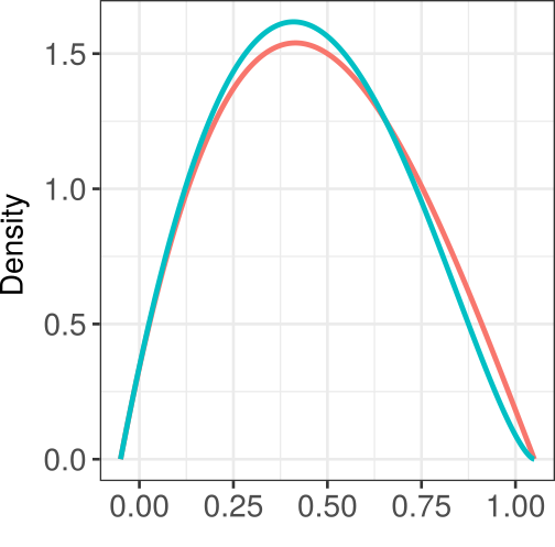
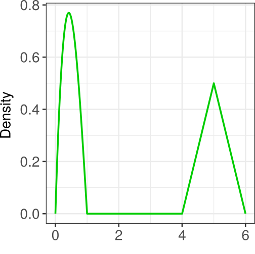
In many applications it is natural to model the objects at hand as compact subsets of $\mathbb{R}^{2}$ or $\mathbb{R}^{3}$ and to equip them with the Euclidean metric and the uniform distribution on the respective sets. Hence, the distributions of distances of these metric measure spaces deserve special attention. Before we can state the next result, which provides simpler conditions than 1.2 and 1.3 in this setting, we have to introduce some notation.
Let $A\subset\mathbb{R}^{d}$ , $d\geq 2$ be a bounded Borel set and let $\lambda^{d}$ denote the Lebesgue measure in $\mathbb{R}^{d}$ . Let $\mathbb{S}_{d-1}$ stand for the unit sphere in $\mathbb{R}^{d}$ . Then, $y\in\mathbb{R}^{d}$ is determined by its polar coordinates $(t,v)$ , where $t=\left\|y\right\|_{2}$ and $v\in\mathbb{S}_{d-1}$ is the unit length vector $y/t$ . Thus, we define the covariance function (Stoyan et al. 2008, Sec. 3.1) for $y=tv\in\mathbb{R}^{d}$ as

K_{A}(t,v)=K_{A}(y)=\lambda^{d}\left(A\cap(A-y)\right),

where $A-y=\left\{a-y:a\in A\right\}$ , and introduce the isotropized set covariance function (Stoyan et al. 2008, Sec. 3.1)

k_{A}(t)=\frac{1}{(\lambda^{d}(A))^{2}}\int_{\mathbb{S}_{d-1}}\!K_{A}(t,v)\,dv.

Furthermore, we define the diameter of a metric space $\left(\mathcal{X},d_{\mathcal{X}}\right)$ as $\mathrm{diam}\left(\mathcal{X}\right)=\sup\{d_{\mathcal{X}}(x_{1},x_{2}):x_{1},x_{2}\in\mathcal{X}\}$ .

Lemma 2.3.

Let $\mathcal{X}\subset\mathbb{R}^{d}$ , $d\geq 2$ , be a compact Borel set, $d_{\mathcal{X}}$ the Euclidean metric and $\mu_{\mathcal{X}}$ the uniform distribution on $\mathcal{X}$ . Let $\mathrm{diam}\left(\mathcal{X}\right)=D$ .

(i)

If $k_{\mathcal{X}}$ is strictly positive on $[0,D)$ , then the induced metric measure space $\left(\mathcal{X},d_{\mathcal{X}},\mu_{\mathcal{X}}\right)$ meets the requirements of 1.2 for any $\beta\in(0,1/2)$ .
(ii)
If additionally there exists $\epsilon>0$ and $\eta>0$ such that
1. 1.
  
  the function $k_{\mathcal{X}}$ is monotonically decreasing on $(D-\epsilon,D)$ ;
2. 2.
  
  we have $k_{\mathcal{X}}(t)\geq c_{\mathcal{X}}(D-t)^{\eta}$ for $t\in(D-\epsilon,D)$ , where $c_{\mathcal{X}}$ denotes a finite, positive constant,
then $\left(\mathcal{X},d_{\mathcal{X}},\mu_{\mathcal{X}}\right)$ also fulfills the requirements of 1.3.

The full proof of the above lemma is deferred to Section B.1 of Weitkamp et al. 2019.

2.2 The Case $DoD_{(0)}=0$

Throughout this subsection we assume that the distribution of distances of the two considered metric measure spaces $\left(\mathcal{X},d_{\mathcal{X}},\mu_{\mathcal{X}}\right)$ and $\left(\mathcal{Y},d_{\mathcal{Y}},\mu_{\mathcal{Y}}\right)$ are equal, i.e., that $\mu^{U}=\mu^{V}$ . Assume that $X_{1},\dots,X_{n}\overset{i.i.d.}{\sim}\mu_{\mathcal{X}}$ and $Y_{1},\dots,Y_{m}\overset{i.i.d.}{\sim}\mu_{\mathcal{Y}}$ are two independent samples. The next theorem states that $\widehat{DoD}_{(\beta)}$ , based on these samples, converges, appropriately scaled, in distribution to the integral of a squared Gaussian process. The case $\beta\in(0,1/2)$ is considered in part $(i)$ , whereas the case $\beta=0$ is considered in part $(ii)$ .

Theorem 2.4.

Assume 1.1 and suppose that $\mu^{U}=\mu^{V}$ .

(i)

Let 1.2 be met and let $m,n\to\infty$ such that ${n}/({n+m})\to\lambda\in\left(0,1\right)$ . Then, it follows

\displaystyle\frac{nm}{n+m}\int_{\beta}^{1-\beta}\!\left(U_{n}^{-1}(t)-V_{m}^{-1}(t)\right)^{2}\,dt\rightsquigarrow\Xi\coloneqq\int_{\beta}^{1-\beta}\!\mathbb{G}^{2}(t)\,dt,

where $\mathbb{G}$ is a centered Gaussian process with covariance

\mathrm{Cov}\left(\mathbb{G}(t),\mathbb{G}(t^{\prime})\right)\!=\!\frac{4}{(u\circ U^{-1}(t))(u\circ U^{-1}(t^{\prime}))}\Gamma_{d_{\mathcal{X}}}(U^{-1}(t),U^{-1}(t^{\prime})).\\

(14)

Here,

	$\displaystyle\Gamma_{d_{\mathcal{X}}}\left(t,t^{\prime}\right)=\int\!\int\!\mathds{1}_{\left\{d_{\mathcal{X}}(x,y)\leq t\right\}}\,d\mu_{\mathcal{X}}(y)\int\!\mathds{1}_{\left\{d_{\mathcal{X}}(x,y)\leq t^{\prime}\right\}}\,d\mu_{\mathcal{X}}(y)\,d\mu_{\mathcal{X}}(x)$
	$\displaystyle-\int\!\int\mathds{1}_{\left\{d_{\mathcal{X}}(x,y)\leq t\right\}}\,d\mu_{\mathcal{X}}(y)\,d\mu_{\mathcal{X}}(x)\int\!\int\!\mathds{1}_{\left\{d_{\mathcal{X}}(x,y)\leq t^{\prime}\right\}}\,d\mu_{\mathcal{X}}(y)\,d\mu_{\mathcal{X}}(x).$

(ii)

If we assume 1.3 instead of 1.2, then the analogous statement holds for the untrimmed version, i.e., for $\beta=0$ .

The main ideas for the proof of 2.4 are illustrated in Appendix A and the full proof can be found in the supplementary material (Weitkamp et al. 2019, Sec. B.2).

Example 2.5.

Recall 2.1, i.e., $\mathcal{X}$ is the unit square in $\mathbb{R}^{2}$ , $d_{\mathcal{X}}$ is the distance induced by the supremum norm and $\mu_{\mathcal{X}}$ is the uniform distribution on $\mathcal{X}$ . Let $X,X^{\prime}\overset{i.i.d.}{\sim}\mu_{\mathcal{X}}$ . From (13), we obtain

U_{1}(t)=\mathbb{P}\left(\left\|X-X^{\prime}\right\|_{\infty}\leq t\right)=\begin{cases}0,&\mathrm{if}~t\leq 0\\ \left(2t-t^{2}\right)^{2},&\mathrm{if}~0\leq t\leq 1\\ 1,&t\geq 1.\end{cases}

Hence, in order to obtain an explicit expression of the covariance structure in the present setting, it remains to determine the first term of $\Gamma_{d_{\mathcal{X}}}$

	$\displaystyle\Gamma_{d_{\mathcal{X}},1}(t,t^{\prime})$	$\displaystyle\coloneqq\int\!\int\!\mathds{1}_{\left\{d_{\mathcal{X}}(x,y)\leq t\right\}}\,d\mu_{\mathcal{X}}(y)\int\!\mathds{1}_{\left\{d_{\mathcal{X}}(x,y)\leq t^{\prime}\right\}}\,d\mu_{\mathcal{X}}(y)\,d\mu_{\mathcal{X}}(x)$
		$\displaystyle=\begin{cases}\left(-\frac{1}{3}t^{\prime 3}-t^{\prime 2}t-2t^{\prime}t^{2}+4t^{\prime}t\right)^{2},&\mathrm{if}~t^{\prime}\leq t<1/2\\ \left(-\frac{1}{3}t^{\prime 3}-t^{\prime 2}t-2t^{\prime}t^{2}+4t^{\prime}t\right)^{2},&\!\begin{aligned} \mathrm{if}~&t^{\prime}<1/2\leq t,\\ ~&t^{\prime}\leq 1-t\end{aligned}\\ \left(-(t^{\prime}-t)^{2}-t^{\prime}t^{2}+t^{\prime}+\frac{1}{3}t^{3}+t-\frac{1}{3}\right)^{2},&\!\begin{aligned} \mathrm{if}~&t^{\prime}<1/2\leq t,\\ ~&t^{\prime}>1-t\end{aligned}\\ \left(-(t^{\prime}-t)^{2}-t^{\prime}t^{2}+t^{\prime}+\frac{1}{3}t^{3}+t-\frac{1}{3}\right)^{2},&\mathrm{if}~1/2\leq t^{\prime}\leq t\leq 1.\end{cases}$

Based on the limit distribution derived in 2.4 it is possible to construct an asymptotic level $\alpha$ test using (estimates of) the theoretical $1-\alpha$ quantiles of $\Xi$ , denoted as $\xi_{1-\alpha}$ , in (12). However, in order to study its finite sample bias, the following bound is helpful (for its proof see Section A.1 and Weitkamp et al. 2019).

Theorem 2.6.

Let $\beta\in[0,1/2)$ , let 1.1 be met and suppose that $\mu^{U}=\mu^{V}$ . Further, let

J_{2}\left(\mu^{U}\right)=\int_{-\infty}^{\infty}\!\frac{U(t)(1-U(t))}{u(t)}\,dt<\infty.

Then it holds for $m,n\geq 3$ that

\mathbb{E}\left[\widehat{DoD}_{(\beta)}\right]\leq\left(\frac{8}{n+1}+\frac{8}{m+1}\right)J_{2}(\mu^{U}).

For instance in the setting of 2.5 it holds $J_{2}\left(\mu^{U}\right)=\frac{5}{48}<\infty$ and thus $\mathbb{E}\left[\widehat{DoD}_{(\beta)}\right]\leq\frac{5}{6}\left(\frac{1}{n+1}+\frac{1}{m+1}\right)$ for $m,n\geq 3$ .

2.3 The Case ${{\bm{DoD_{(0)}>0$}}}$

Inthissubsection,weareconcernedwiththebehaviorof ^ DoD _(β) $giventhatthedistributionsofdistancesofthemetricmeasurespaces$ (X,d_X,μ_X) $and$ (Y,d_Y,μ_Y) $donotcoincide.Justasfor\lx@cref{creftypecap\lx@tilde refnum}{thm:main2},wedistinguishthecases$ β∈(0,1/2) $and$ β= 0 $.\begin{thm}Assume \lx@cref{creftypecap\lx@tilde refnum}{cond:setting}. \begin{itemize}\itemize@item@[(i)]Assume that \lx@cref{creftypecap\lx@tilde refnum}{cond:firstcondition} holds, let $m,n\to\infty$ such that $\frac{n}{n+m}\to\lambda\in\left(0,1\right)$ and let $DoD_{(\beta)}>0$. Then, it follows that $$\sqrt{\frac{nm}{n+m}}\left(\widehat{DoD}_{(\beta)}-DoD_{(\beta)}\right)$$converges in distribution to a normal distribution with mean 0 and variance \@@amsalign Here, $\Gamma_{d_{\mathcal{X}}}\left(x,y\right)$ is as defined in \lx@cref{creftypecap\lx@tilde refnum}{thm:main2} and $\Gamma_{d_{\mathcal{Y}}}\left(x,y\right)$ is defined analogously. \par\vskip 4.0pt\vskip 4.0pt plus 2.0pt minus 1.0pt\itemize@item@[(ii)]If we assume \lx@cref{creftypecap\lx@tilde refnum}{cond:secondcondition} instead of \lx@cref{creftypecap\lx@tilde refnum}{cond:firstcondition}, then the analogous statement holds for the untrimmed version, i.e., for $\beta=0$. \end{itemize}\end{thm}Theproofof\lx@cref{creftypecap\lx@tilde refnum}{thm:main}issketchedin\lx@cref{creftypecap\lx@tilde refnum}{appendix:proofs}.AdetailedversionisgiveninSectionB.4of\cite[cite]{\@@bibref{Authors Phrase1YearPhrase2}{supplement}{\@@citephrase{(}}{\@@citephrase{)}}}.\begin{rem}The assumptions of \lx@cref{creftypecap\lx@tilde refnum}{thm:main} $(i)$ include that $\beta$ is chosen such that \begin{equation*}DoD_{(\beta)}>0.\end{equation*}Suppose on the other hand that $\mu^{U}\neq\mu^{V}$, but $DoD_{(\beta)}=0$, i.e., their quantile functions agree Lebesgue almost surely on the considered interval $[\beta,1-\beta]$. Then, the limits found in \lx@cref{creftypecap\lx@tilde refnum}{thm:main} are degenerate and it is easy to verify along the lines of the proof of \lx@cref{creftypecap\lx@tilde refnum}{thm:main2} that $\widehat{DoD}_{(\beta)}$ exhibits the same distributional limit as in the case $DoD_{(0)}=0$. \end{rem}\begin{rem}So far we have restricted ourselves to the case $p=2$. However, most of our findings directly translate to results for the statistic $\widehat{{DoD}}_{p}$, $p\in[1,\infty)$, defined in \eqref{eq:introlowerboundempversion}. Using the same ideas one can directly derive \lx@cref{creftypecap\lx@tilde refnum}{thm:main2} and \lx@cref{creftypecap\lx@tilde refnum}{thm:finite sample bound for p=2} for (a trimmed version) of $\widehat{{DoD}}_{p}$ (see Sections B.2 and B.3 of \cite[citet]{\@@bibref{Authors Phrase1YearPhrase2}{supplement}{\@@citephrase{(}}{\@@citephrase{)}}}) under slightly different assumptions. Only the proof of \lx@cref{creftypecap\lx@tilde refnum}{thm:main} requires more care (see \cite[cite]{(\@@bibref{AuthorsPhrase1Year}{supplement}{\@@citephrase{, }}{}, Sec. B.4)}). \end{rem}\par\par\par\par\par$

3 Bootstrapping the Quantiles

The quantiles of the limit distribution of $\widehat{DoD}_{(\beta)}$ under $H_{0}$ depend on the unknown distribution $U$ and are therefore in general not accessible. One possible approach, which is quite cumbersome, is to estimate the covariance matrix of the Gaussian limit process $G$ from the data and use this to approximate the quantiles required. Alternatively, we suggest to directly bootstrap the quantiles of the limit distribution of $\widehat{DoD}_{(\beta)}$ under $H_{0}$ . To this end, we define and investigate the bootstrap versions of $U_{n}$ , $U_{n}^{-1}$ and $\mathbb{U}_{n}^{-1}\coloneqq\sqrt{n}\left(U_{n}^{-1}-U^{-1}\right)$ .

Let $\mu_{n}$ denote the empirical measure based on the sample $X_{1},\dots,X_{n}$ . Given the sample values, let ${X}_{1}^{*},\dots,{X}_{n_{B}}^{*}$ be an independent identically distributed sample of size $n_{B}$ from $\mu_{n}$ . Then, the bootstrap estimator of $U_{n}$ is defined as

\displaystyle{U}_{n_{B}}^{*}(t):=\frac{2}{n_{B}(n_{B}-1)}\sum_{1\leq i<j\leq n_{B}}\mathds{1}_{\left\{d_{\mathcal{X}}({X}_{i}^{*},{X}_{j}^{*})\leq t\right\}},

the corresponding bootstrap empirical $U$ -process is for $t\in\mathbb{R}$ given as ${\mathbb{U}}_{n_{B}}^{*}(t)=\sqrt{n_{B}}\big({U}_{n_{B}}^{*}(t)-U_{n}(t)\big)$ and the corresponding bootstrap quantile process for $t\in(0,1)$ as $\left({\mathbb{U}}_{n_{B}}^{*}\right)^{-1}(t)=\sqrt{n_{B}}\Big(\big({U}_{n_{B}}^{*}\big)^{-1}(t)-U_{n}^{-1}(t)\Big)$ .
One can easily verify along the lines of the proof of 2.4 that for $n\to\infty$ it also holds for $\beta\in(0,1/2)$

\int_{\beta}^{1-\beta}\!\left(\mathbb{U}_{n}^{-1}(t)\right)^{2}\,dt\rightsquigarrow\Xi=\int_{\beta}^{1-\beta}\!\mathbb{G}^{2}(t)\,dt.

(15)

Hence, this suggests to to approximate the quantiles of $\Xi$ by the quantiles of its bootstrapped version

{\Xi}_{n_{B}}^{*}\coloneqq\int_{\beta}^{1-\beta}\!\left(\left({\mathbb{U}}_{n_{B}}^{*}\right)^{-1}(t)\right)^{2}\,dt.

(16)

Let $\beta\in(0,1/2)$ , suppose that 1.2 holds, let $\sqrt{n_{B}}=o(n)$ and let $\xi_{n_{B},\alpha}^{(R)}$ denote the empirical bootstrap quantile of $R$ independent bootstrap realizations ${\Xi}_{n_{B}}^{*,(1)},\dots,{\Xi}_{n_{B}}^{*,(R)}$ . Under these assumptions, we derive (cf. Section C of the supplement Weitkamp et al. 2019) that for any $\alpha\in(0,1)$ it follows

\lim_{n,n_{B},R\to\infty}\mathbb{P}\left(\int_{\beta}^{1-\beta}\!\left(\mathbb{U}_{n}^{-1}(t)\right)^{2}\,dt\geq\xi_{n_{B},\alpha}^{(R)}\right)=\alpha.

(17)

Because of (15) the statement (17) guarantees the consistency of $\xi_{n_{B},\alpha}^{(R)}$ for $n,n_{B},R\to\infty$ . Hence, a consistent bootstrap analogue of the test defined by the decision rule (12) is for $\beta\in(0,1/2)$ given by the bootstrapped Distribution of Distances (DoD)-test

\Phi_{DoD}^{*}(\mathcal{X}_{n},\mathcal{Y}_{m})=\begin{cases}1,&\text{if}~\frac{nm}{n+m}\widehat{DoD}_{(\beta)}>\xi_{n_{B},1-\alpha}^{(R)}\\ 0,&\text{if}~\frac{nm}{n+m}\widehat{DoD}_{(\beta)}\leq\xi_{n_{B},1-\alpha}^{(R)}.\end{cases}

(18)

4 Simulations

We investigate the finite sample behavior of $\widehat{DoD}_{(\beta)}$ in Monte Carlo simulations. To this end, we simulate the speed of convergence of $\widehat{DoD}_{(\beta)}$ under $H_{0}$ to its limit distribution (2.4) and its behavior under $H_{1}$ . Moreover, we showcase the accuracy of the approximation by the bootstrap scheme introduced in Section 3 and investigate what kind of differences are detectable in the finite sample setting using the bootstrapped DoD-test $\Phi_{DoD}^{*}$ defined in (18). All simulations were performed using $\mathsf{R}$ (R Core Team 2017).

4.1 The Hypothesis

We begin with the simulation of the finite sample distribution under the hypothesis and consider the metric measure space $\left(\mathcal{X},d_{\mathcal{X}},\mu_{\mathcal{X}}\right)$ from 2.1, where $\mathcal{X}$ denotes the unit square in $\mathbb{R}^{2}$ , $d_{\mathcal{X}}$ the distance induced by the supremum norm and $\mu_{\mathcal{X}}$ the uniform distribution on $\mathcal{X}$ . We generate for $n=m=10,50,100,250$ two samples $\mathcal{X}_{n}$ and $\mathcal{X}_{n}^{\prime}$ of $\mu_{\mathcal{X}}$ and calculate for $\beta=0.01$ the statistic $\frac{n}{2}\widehat{DoD}_{(\beta)}$ . For each $n$ , we repeat this process 10.000 times. The finite sample distribution is then compared to a Monte Carlo sample of its theoretical limit distribution (sample size 10.000). Kernel density estimators (Gaussian kernel with bandwidth given by Silverman’s rule) and Q-Q-plots are displayed in Figure 4. All plots highlight that the finite sample distribution of $\widehat{DoD}_{(\beta)}$ is already well approximated by its theoretical limit distribution for moderate sample sizes. Moreover, for $n=10$ the quantiles of the finite sample distribution of $\widehat{DoD}_{(\beta)}$ are in general larger than the ones of the sample of its theoretical limit distribution, which suggests that the DoD-test will be rather conservative for small $n$ . For $n\geq 50$ most quantiles of the finite sample distribution of $\widehat{DoD}_{(\beta)}$ match the ones of its theoretical limit distribution reasonably well.

4.2 Alternative

Next we investigate the behavior of the statistic $\widehat{DoD}_{(\beta)}$ under the alternative. To this end, we consider the metric measure spaces $\left(\mathcal{X},d_{\mathcal{X}},\mu_{\mathcal{X}}\right)$ and $\left(\mathcal{Y},d_{\mathcal{Y}},\mu_{\mathcal{Y}}\right)$ , where $\left(\mathcal{X},d_{\mathcal{X}},\mu_{\mathcal{X}}\right)$ denotes the one as defined in Section 4.1 and $\left(\mathcal{Y},d_{\mathcal{Y}},\mu_{\mathcal{Y}}\right)$ the one, where $\mathcal{Y}$ is a disc in $\mathbb{R}^{2}$ with radius 0.5, $d_{\mathcal{Y}}$ the distance induced by the supremum norm and $\mu_{\mathcal{Y}}$ the uniform distribution on $\mathcal{Y}$ . From a testing point of view it is more interesting to compare the finite sample distribution under the alternative to the limit distribution under $H_{0}$ (the considered metric measure spaces are isomorphic) than to investigate the speed of convergence to the limit derived in . Thus, we repeat the course of action of Section 4.1 for $n=m=10,50,100,250$ and $\beta=0.01$ with samples $\mathcal{X}_{n}$ and $\mathcal{Y}_{n}$ from $\mu_{\mathcal{X}}$ and $\mu_{\mathcal{Y}}$ , respectively.
In order to highlight the different behavior of $\widehat{DoD}_{(\beta)}(\mathcal{X}_{n},\mathcal{Y}_{n})$ in this setting, we compare its finite sample distributions to the theoretical limit distribution under the hypothesis, which has already been considered in Section 4.1.
The results are visualized as kernel density estimators (Gaussian kernel with bandwidth given by Silverman’s rule) and Q-Q-plots in Figure 5. As $n$ grows, the kernel density estimator based on the realizations of $\widehat{DoD}_{(\beta)}(\mathcal{X}_{n},\mathcal{Y}_{n})$ shifts to the right and becomes less and less concentrated. Furthermore, it becomes more and more symmetric around its peak which matches its theoretical Gaussian limit behavior (recall ). For $n\geq 100$ we see in Figure 5 that the densities based on the realizations of $\widehat{DoD}_{(\beta)}(\mathcal{X}_{n},\mathcal{Y}_{n})$ differ drastically from the ones based on the Monte Carlo samples of the theoretical limit distribution under $H_{0}$ . The corresponding Q-Q-plots underline this observation and highlight that for $n\geq 50$ essentially all quantiles of the sample are drastically larger than the ones of the theoretical limit distribution. This suggests that the proposed test discriminates between these metric measure spaces with high probability already for moderate values of $n$ .

4.3 The Bootstrap Test

We now investigate the finite sample properties of the bootstrap test $\Phi_{DoD}^{*}$ (defined in (18)). Therefore, we compare the metric measure space $\left(\mathcal{V},d_{\mathcal{V}},\mu_{\mathcal{V}}\right)$ , where $\mathcal{V}$ is the unit square, $d_{\mathcal{V}}$ is the Euclidean distance and $\mu_{\mathcal{V}}$ the uniform distribution on $\mathcal{V}$ , with the spaces $\left\{\left(\mathcal{W}_{i},d_{\mathcal{W}_{i}},\mu_{\mathcal{W}_{i}}\right)\right\}_{i=1}^{5}$ . Here, $\mathcal{W}_{i}$ denotes the intersection of the unit square with a disc of radius $r_{i}\in\left\{\sqrt{2}/2,0.65,0.6,0.55,0.5\right\}$ both centered at $(0,0)$ , $d_{\mathcal{W}_{i}}$ the Euclidean distance and $\mu_{\mathcal{W}_{i}}$ the uniform distribution on $\mathcal{W}_{i}$ . In Figure 6 the sets $\mathcal{V}$ (white) and $\left\{\mathcal{W}_{i}\right\}_{i=1}^{5}$ (red) are displayed. It highlights the increasing similarity of the sets for growing $r_{i}$ .

(a)

r_{1}=\frac{\sqrt{2}}{2}

(b)

r_{2}=0.65

(c)

r_{3}=0.6

(d)

r_{4}=0.55

(e)

r_{5}=0.5

Figure 6: Different metric measure spaces: Comparisons of the metric measure space

\left(\mathcal{V},d_{\mathcal{V}},\mu_{\mathcal{V}}\right)

(white) to the spaces

\left\{\left(\mathcal{W}_{i},d_{\mathcal{W}_{i}},\mu_{\mathcal{W}_{i}}\right)\right\}_{i=1}^{5}

(red).

Before we employ the bootstrap DoD-test with $\beta=0.01$ in the present setting, we consider the bootstrap approximation proposed in Section 3 in this simple setting. Therefore, we generate $n=10,50,100,250$ realizations of $\mu_{\mathcal{V}}$ and calculate for $n_{B}=n$ based on these samples 1000 times

{\Xi}_{n_{B}}^{*}=\int_{0.01}^{0.99}\!\left(\left({\mathbb{U}}_{n_{B}}^{*}\right)^{-1}(t)\right)^{2}\,dt

as described in Section 3. We then compare for the different $n$ the obtained finite sample distributions to ones of $\widehat{DoD}_{(\beta)}(\mathcal{V}_{n},\mathcal{W}_{1,n})$ (generated as described in Section 4.1).

The results are summarized as kernel density estimators (Gaussian kernel with bandwidth given by Silverman’s rule) and Q-Q-plots in Figure 7. Both, the kernel density estimators and the Q-Q-plots show that for $n\leq 50$ the bootstrap quantiles are clearly larger than the empirical quantiles leading to a rather conservative procedure for smaller $n$ , an effect that disappears for large $n$ .

Next, we aim to apply $\Phi_{DoD}^{*}$ for $\beta=0.01$ at $5\%$ -significance level for discriminating between $\left(\mathcal{V},d_{\mathcal{V}},\mu_{\mathcal{V}}\right)$ and each of the spaces $\left(\mathcal{W}_{i},d_{\mathcal{W}_{i}},\mu_{\mathcal{W}_{i}}\right)$ , $i=1,\dots,5$ . To this end, we bootstrap the quantile $\xi_{0.95}$ based on samples from $\mu_{\mathcal{V}}$ as described in Section 3 ( $R=1000$ ) and then we apply the test $\Phi_{DoD}^{*}$ , defined in (18), with the bootstrapped quantile $\xi_{n_{B},\alpha}^{(R)}$ on 1000 samples of size $n=10,50,100,250,500,$ $1000$ as illustrated in Section 3. The results are summarized in Table 1. In accordance to the previous simulations, we find that the prespecified significance level (for $r_{1}=\sqrt{2}/2$ the sets are equal) is approximated well for $n\geq 100$ . Concerning the power of the test we observe that it is conservative for small $n$ , but already for $n\geq 100$ the cases (d) and (e) (see Figure 6) are detected reasonably well. If we choose $n=1000$ , even the spaces in (c) are distinguishable, although in this case, $\mathcal{W}_{3}$ fills out about $94\%$ of $\mathcal{V}$ . For (b), i.e., $r_{2}=0.65$ , where more than $98\%$ of $\mathcal{V}$ is covered by $\mathcal{W}_{4}$ , the power of the test falls below $0.11$ .

$\Phi_{DoD}^{*}$
Sample Size	$r_{1}={\sqrt{2}}/{2}$	$r_{2}=0.65$	$r_{3}=0.6$	$r_{4}=0.55$	$r_{5}=0.5$
10	0.010	0.018	0.005	0.006	0.009
50	0.031	0.034	0.041	0.139	0.406
100	0.048	0.048	0.098	0.323	0.824
250	0.038	0.058	0.203	0.722	1.000
500	0.045	0.080	0.402	0.962	1.000
1000	0.051	0.108	0.713	1.000	1.000

Table 1: Comparison of different metric measure spaces I: The empirical power of the DoD-test

\Phi_{DoD}^{*}

(1000 replications) for the comparison of the metric measure spaces represented in Figure 6 for different

n

In order to highlight how much power we gain in the finite sample setting by carefully handling the occurring dependencies we repeat the above comparisons, but calculate $\widehat{DoD}_{(\beta)}$ only based on the independent distances, i.e., on $\{d_{\mathcal{X}}(X_{1},X_{2}),d_{\mathcal{X}}(X_{3},X_{4}),\dots,d_{\mathcal{X}}(X_{n-1},X_{n})\}$ and $\{d_{\mathcal{Y}}(Y_{1},Y_{2}),d_{\mathcal{Y}}(Y_{3},Y_{4}),\dots,d_{\mathcal{Y}}(Y_{m-1},Y_{m})\}$ , instead of all available distances. In the following, the corresponding statistic is denoted as $\widehat{D}_{\beta,ind}$ . From the existing theory on testing with the empirical (trimmed) Wasserstein distance Munk and Czado 1998; del Barrio et al. 1999; del Barrio et al. 2005 it is immediately clear, how to construct an asymptotic level $\alpha$ test $\Phi_{{D}_{ind}}$ based on $\widehat{D}_{\beta,ind}$ . The results for comparing $\left(\mathcal{V},d_{\mathcal{V}},\mu_{\mathcal{V}}\right)$ and $\left\{\left(\mathcal{W}_{i},d_{\mathcal{W}_{i}},\mu_{\mathcal{W}_{i}}\right)\right\}_{i=1}^{5}$ using $\Phi_{{D}_{ind}}$ with $\beta=0.01$ are displayed in Table 2. Apparently, $\Phi_{{D}_{ind}}$ keeps its prespecified significance level of $\alpha=0.05$ , but develops significantly less power than $\Phi_{DoD}^{*}$ in the finite sample setting.

$\Phi_{{D}_{ind}}$
Sample Size	$r_{1}={\sqrt{2}}/{2}$	$r_{2}=0.65$	$r_{3}=0.6$	$r_{4}=0.55$	$r_{5}=0.5$
100	0.036	0.040	0.048	0.050	0.177
250	0.041	0.043	0.043	0.179	0.799
500	0.051	0.045	0.084	0.583	0.998
1000	0.043	0.044	0.231	0.974	1

Table 2: Comparison of different metric measure spaces III: The empirical power of the test based on

\widehat{D}_{\beta,ind}

(1000 applications) for the comparison of the metric measure spaces represented in Figure 6.

Furthermore, we investigate the influence of $\beta$ on our results. To this end, we repeat the previous comparisons with $n=250$ and $\beta=0,0.01,0.05,0.25$ . The results of the corresponding comparisons are displayed in Table 3. It highlights that the test $\Phi_{DoD}^{*}$ holds its level for all $\beta$ . Furthermore, we observe a decrease in power with increasing $\beta$ , i.e., increasing degree of trimming. This is due to the fact that excluding too many large distances will no longer show small differences in the diameter.

$\Phi_{DoD}^{*}$
$\beta$	$r_{1}={\sqrt{2}}/{2}$	$r_{2}=0.65$	$r_{3}=0.6$	$r_{4}=0.55$	$r_{5}=0.5$
0	0.048	0.058	0.228	0.776	0.997
0.01	0.051	0.065	0.232	0.736	0.995
0.05	0.049	0.059	0.189	0.676	0.998
0.25	0.045	0.061	0.156	0.579	0.979

Table 3: The influence of

\beta

: The empirical power of the DoD-test

\Phi_{DoD}^{*}

(1000 replications) for the comparison of the metric measure spaces represented in Figure 6 for different

\beta

To conclude this subsection, we remark that in the above simulations the quantiles required for the applications of $\Phi_{DoD}^{*}$ were always estimated based on samples of $\mu_{\mathcal{V}}$ . Evidently, this slightly affects the results obtained, but we found that this influence is not significant.

5 Structural Protein Comparisons

Next, we apply the DoD-test to compare the protein structures displayed in Figure 2. First, we compare 5D0U with itself, in order to investigate the actual significance level of the proposed test under $H_{0}$ in a realistic example. Afterwards, 5D0U is compared with 5JPT and with 6FAA, respectively. However, before we can apply $\Phi_{DoD}^{*}$ , we need to model proteins as metric measure spaces. Thus, we briefly recap some well known facts about proteins to motivate the subsequent approach. A protein is a polypeptide chain made up of amino acid residues linked together in a definite sequence. Tracing the repeated amide, $C^{\alpha}$ and carbonyl atoms of each amino acid residue, a so called backbone can be identified. It is well established that the distances between the $C^{\alpha}$ atoms of the backbone contain most of the information about the protein’s structure Rossman and Liljas 1974; Kuntz 1975; Jones and Thirup 1986; Holm and Sander 1993. For the following comparisons, we randomly select $n=10,50,100,250,500$ from the 650-750 $C^{\alpha}$ atoms of the respective proteins and assume that the corresponding coordinates are samples of unknown distributions $\left\{\mu_{\mathcal{X}_{i}}\right\}_{i=1}^{3}$ supported on Borel sets $\mathcal{X}_{i}\subset\mathbb{R}^{3}$ equipped with the Euclidean distance. Furthermore, we choose $\beta=0.01$ , $\alpha=0.05$ and determine for each $n$ the bootstrap quantile $\xi_{n_{B},0.95}^{(R)}$ based on a sample of size $n$ from 5D0U ( $R=1000$ , $n_{B}=n$ ) as illustrated in Section 3. This allows us to directly apply the test ${\Phi}_{DoD}^{*}$ on the drawn samples.

The results of our comparisons are summarized in Figure 8. It displays the empirical significance level resp. the empirical power of the proposed method as a function of $n$ .

5D0U vs 5D0U: In accordance with the previous simulation study this comparison (see Figure 8, left) shows that $\Phi_{DoD}^{*}$ is conservative in this application as well.

5D0U vs 5JPT: We have already mentioned in Section 1.3 that 5D0U and 5JPT are structures of the same protein extracted from two different organisms and thus highly similar (their alignment has a root mean deviation of less than 0.59 Å). The empirical power for this comparison (Figure 8, middle) stays for all $n$ below $\alpha=0.05$ and thus the test does not discriminate between these two protein structures in accordance with our biological knowledge.

5D0U vs 6FAA: Although the protein structures 5D0U and 6FAA are similar at large parts (their alignment has a root mean square deviation of $0.75$ Å), the DoD-test is able to discriminate between them with high statistical power. The empirical power (Figure 8, right) is a strictly monotonically increasing function in $n$ that is greater than 0.63 for $n\geq 100$ and approaches 1 for $n=500$ (recall that we use random samples of the $650-750$ $C^{\alpha}$ atoms).

Figure 8: Protein Structure Comparison: Empirical significance level for comparing 5D0U with itself (left), empirical power for the comparison of 5D0U with 5JPT (middle) as well as the the empirical power for comparing 5D0U with 6FAA (right). 1000 repetitions of the test

{\Phi}^{*}_{DoD}

have been simulated for each

n

Finally, we remark that throughout this section we have always based the quantiles required for testing on samples of the protein structure 5D0U. By the definition of $\Phi_{DoD}^{*}$ it is evident that this influences the results. If we compared the proteins 6FAA and 5D0U using $\Phi_{DoD}^{*}$ with quantiles obtained by a sample of 6FAA, the results would change slightly, but remain comparable.

5.1 Comparison to the DTM-test

In this section, we investigate how the test proposed by Brécheteau 2019 compares to $\Phi_{DoD}^{*}$ for protein structure comparison. To put this method in our context, we briefly introduce the method proposed in the latter reference, comment on the underlying theoretical signature and compare the empirical power of the two tests in some simple scenarios.

We begin with the introduction of the empirical distance to measure signature. Let $\left(\mathcal{X},d_{\mathcal{X}},\mu_{\mathcal{X}}\right)$ be a metric measure space with $X_{1},\dots,X_{n}\overset{i.i.d.}{\sim}\mu_{\mathcal{X}}$ and let $\mathcal{X}_{n}=\left\{X_{1},\dots,X_{n}\right\}$ . Then, the (empirical) distance to measure function with mass parameter $\kappa={k}/{n}$ is given as

\delta_{\mathcal{X}_{n},\kappa}(x)\coloneqq\frac{1}{k}\sum_{i=1}^{k}d_{\mathcal{X}}\left(X^{(i)},x\right),

where $X^{(i)}$ denotes the $i$ ’th nearest neighbor of $x$ in the sample $\mathcal{X}_{n}$ (for general $\kappa$ see Brécheteau 2019). For $n_{S}\leq n$ the empirical distance to measure signature with mass parameter $\kappa={k}/{n}$ is then defined as

D_{\mathcal{X}_{n},\kappa}\left({n_{S}}\right)\coloneqq\frac{1}{n_{S}}\sum_{i=1}^{n_{S}}\delta_{\mathcal{X}_{n},\kappa}(X_{i}),

(19)

which is a discrete probability distribution on $\mathbb{R}$ . Let $\left(\mathcal{Y},d_{\mathcal{Y}},\mu_{\mathcal{Y}}\right)$ be a second metric measure space, $Y_{1},\dots,Y_{n}\overset{i.i.d.}{\sim}\mu_{\mathcal{Y}}$ , let $\mathcal{Y}_{n}=\{Y_{1},\dots,Y_{n}\}$ and let $D_{\mathcal{Y}_{n},\kappa}\left({n_{S}}\right)$ be defined analogously to (19). Then, given that $\frac{n_{S}}{n}=o(1)$ , Brécheteau 2019 constructs an asymptotic level $\alpha$ test for $H_{0}$ defined in (3) based on the 1-Kantorovich distance between the respective empirical distance to measure signatures, i.e., on the test statistic

T_{n_{S},\kappa}(\mathcal{X}_{n},\mathcal{Y}_{n})\coloneqq\mathcal{K}_{1}\left(D_{\mathcal{X}_{n},\kappa}\left({n_{S}}\right),D_{\mathcal{Y}_{n},\kappa}\left({n_{S}}\right)\right).

(20)

The corresponding test, that rejects if (20) exceeds a bootstrapped critical value $q^{DTM}_{\alpha}$ , is in the following denoted as $\Phi_{DTM}$ . The test statistic $T_{n_{S},\kappa}$ is related to the Gromov-Kantorovich distance as follows (see (Brécheteau 2019, Prop. 3.2))

T_{\kappa}(\mathcal{X},\mathcal{Y})\coloneqq\mathcal{K}_{1}(D_{\mathcal{X},\kappa},D_{\mathcal{Y},\kappa})\leq\frac{2}{\kappa}\mathcal{GK}_{1}\left(\mathcal{X},\mathcal{Y}\right).

Here, $D_{\mathcal{X},\kappa}$ and $D_{\mathcal{Y},\kappa}$ denote the true distance to measure signature (see (Brécheteau 2019, Sec. 1) or Section B.6 in the supplementary material Weitkamp et al. 2019 for a formal definition) of $\left(\mathcal{X},d_{\mathcal{X}},\mu_{\mathcal{X}}\right)$ and $\left(\mathcal{Y},d_{\mathcal{Y}},\mu_{\mathcal{Y}}\right)$ , respectively.

The first step for the comparison of both methods is now to analyze how the respective signatures, the distribution of distances and the distance to measure signature, relate to each other. By the definition of $D_{\mathcal{X},\kappa}$ , which coincides for $n=n_{S}$ with (19) for discrete metric measure spaces with $n$ points and the uniform measure, we see that $T_{\kappa}(\mathcal{X},\mathcal{Y})$ puts emphasis on local changes. This allows it to discriminate between the metric measure spaces in Figure 7 of Mémoli 2011 for $\kappa>1/4$ , whereas $DoD_{p}\left(\mathcal{X},\mathcal{Y}\right)$ is always zero for this example. One the other hand, for $\kappa\leq 1/2$ , $T_{\kappa}(\mathcal{X},\mathcal{Y})$ cannot distinguish between the metric measure spaces displayed in Figure 9, whereas $DoD_{p}(\mathcal{X},\mathcal{Y})$ can become arbitrarily large, if the represented triangles are moved further apart. More precisely, $DoD_{p}$ scales as the $p$ ’th power of the distance between the triangles.

Figure 9: Different metric measure spaces: Representation of two different, discrete metric measure spaces that are both equipped with the respective uniform distribution. Left: Three points with the same pairwise distances (dash-dotted lines). Right: Two translated copies that are further than one side length apart.

Generally, one can show that $DoD_{p}(\mathcal{X},\mathcal{Y})$ and $T_{\kappa}(\mathcal{X},\mathcal{Y})$ are related to different sequences of lower bounds for the Gromov-Kantorovich distance (see (Weitkamp et al. 2019, Sec. B.6) for more details).

The next step of the comparison of both methods consists in comparing their performance for simulated examples. To this end, we repeat the comparisons of $\left(\mathcal{V},d_{\mathcal{V}},\mu_{\mathcal{V}}\right)$ with the spaces $\left\{\left(\mathcal{W}_{i},d_{\mathcal{W}_{i}},\mu_{\mathcal{W}_{i}}\right)\right\}_{i=1}^{5}$ as done in Section 4.3. Furthermore, we simulate the empirical power of $\Phi_{DoD}^{*}$ in the setting of Section 4.2 of Brécheteau 2019. For both comparisons, we choose a significance level of $\alpha=0.05$ . We begin with applying $\Phi_{DTM}$ in the setting of Section 4.3. By the definition of the test statistic in (20) and the representation of the metric measure spaces in Figure 6, it is clear that this setting is difficult for the method based on $T_{n_{S},\kappa}$ . Furthermore, we remark that the test $\Phi_{DTM}$ is not easily applied in the finite sample setting. Although it is an asymptotic test of level $\alpha$ , the parameters $n_{S}$ and $\kappa$ have to be chosen carefully for the test to hold its prespecified significance level for finite samples. In particular, choosing $n_{S}$ and $\kappa$ large violates the independence assumption underlying the results of Brécheteau 2019.
Generally, we found that the choices $\kappa\leq 0.1$ and $n_{S}\leq n/15$ yield reasonable results which we list in Table 4. The results show that the DTM-test holds its significance level (for $r_{1}$ both spaces are the same) and develops a significant amount of power for the cases $r_{4}$ and $r_{5}$ . As to be expected it struggles to discriminate $\left(\mathcal{V},d_{\mathcal{V}},\mu_{\mathcal{V}}\right)$ and $\left(\mathcal{W}_{3},d_{\mathcal{W}_{3}},\mu_{\mathcal{W}_{3}}\right)$ , as for this task especially the large distances are important. Here, $\Phi_{DoD}^{*}$ clearly outperforms $\Phi_{DTM}$ .

$\kappa=0.05$ , $\alpha=0.05$
Sample Size	$r_{1}={\sqrt{2}}/{2}$	$r_{2}=0.65$	$r_{3}=0.6$	$r_{4}=0.55$	$r_{5}=0.5$
100	0.039	0.054	0.049	0.064	0.096
250	0.053	0.049	0.070	0.144	0.379
500	0.065	0.076	0.128	0.361	0.853
1000	0.072	0.088	0.259	0.740	1
$\kappa=0.1$ , $\alpha=0.05$
Sample Size	$r_{1}={\sqrt{2}}/{2}$	$r_{2}=0.65$	$r_{3}=0.6$	$r_{4}=0.55$	$r_{5}=0.5$
100	0.067	0.047	0.070	0.083	0.170
250	0.066	0.069	0.094	0.163	0.533
500	0.064	0.081	0.147	0.430	0.926
1000	0.064	0.091	0.255	0.790	1

Table 4: Comparison of different metric measure spaces II: The empirical power of the test based on

T_{n_{S},\kappa}

(1000 applications) for the comparison of the metric measure spaces represented in Figure 6 for different

n

and

\kappa

(

n_{S}=n/15

In a further example, we investigate how well $\Phi_{DoD}^{*}$ and $\Phi_{DTM}$ discriminate between different spiral types (see Figure 10). These spirals are constructed as follows. Let $R\sim U[0,1]$ be uniformly distributed and independent of $S,S^{\prime}\overset{i.i.d.}{\sim}N(0,1)$ . Choose a significance level of $\alpha=0.05$ and let $\beta=0.01$ . For $v=10,15,20,30,40,100$ we simulate samples of

(R\sin(vR)+0.03S,R\cos(vR)+0.03S^{\prime})\sim\mu_{v}

(21)

and considers these to be samples from a metric measure spaces equipped with the Euclidean metric.

Figure 10: Different metric measure spaces II: Representation of samples created by (21) for

v=10,15,20

(from left to right).

We apply $\Phi_{DoD}^{*}$ with quantiles based on $\mu_{v}$ in order to compare $\mu_{v}$ with $\mu_{v}$ (based on different samples) and $\mu_{v}$ with $\mu_{10}$ , $v=15,\dots,100$ . The results presented in Table 5 show that $\Phi_{DoD}^{*}$ holds its significance level and always discriminates between $\mu_{10}$ and $\mu_{v}$ in this setting. The reported values from Brécheteau 2019 are also listed for the ease of readability. They show that the additional subsampling in the definition of (20) leads to a loss of power in this example. Moreover, for $\Phi_{DTM}$ the results always depend on the choice of the parameters.

$\Phi_{DoD}^{*}$
$v$	15	20	30	40	100
Type-I error	0.036	0.051	0.051	0.054	0.048
Emp. power	1	1	1	1	1
$\Phi_{DTM}$
$v$	15	20	30	40	100
Type-I error	0.043	0.049	0.050	0.051	0.050
Emp. power	0.525	0.884	0.987	0.977	0.985

Table 5: Spiral Comparison: Empirical significance level and power of

\Phi_{DoD}^{*}

and

\Phi_{DTM}

for the comparisons the metric measure spaces represented in Figure 10.

Finally, we come to the protein structure comparison. We repeat the previous comparisons of 5D0U, 5JPT and 6FAA for a significance level $\alpha=0.05$ , $n=100,250,500$ , $n_{S}=N/5$ and $\kappa=0.05,0.1$ . The results are reported in Table 6. We see that also $\Phi_{DTM}$ approximately holds its significance level and is more sensitive to small local changes such as slight shifts of structural elements for small $\kappa$ . However, the evident differences between 5D0U and 6FAA are detected much better by ${\Phi}_{DoD}^{*}$ (see Figure 8).

$\kappa=0.05$ , $\alpha=0.05$
$n$	5D0U vs 5D0U	5D0U vs 5JPT	5D0U vs 6FAA
100	0.055	0.068	0.109
250	0.049	0.080	0.297
500	0.037	0.090	0.690
$\kappa=0.1$ , $\alpha=0.05$
$n$	5D0U vs 5D0U	5D0U vs 5JPT	5D0U vs 6FAA
100	0.068	0.061	0.166
250	0.056	0.084	0.420
500	0.047	0.104	0.760

Table 6: Protein Comparison II: The empirical power of the Test proposed by Brécheteau 2019 (1000 applications) for the comparison of proteins represented in Figure 2 for different

n

and

\kappa

(

n_{S}=n/5

5.2 Discussion

We conclude this section with some remarks on the way we have modeled proteins as metric measure spaces in this section. The flexibility of metric measure spaces offers possible refinements which might be of interest for further investigation. For example, we have treated all $C^{\alpha}$ atoms as equally important, although it appears to be reasonable for some applications to put major emphasis on the cores of the proteins. Further, one could have included that the error of measurement that is in general higher for some parts of the protein by adjusting the measure on the considered space accordingly. Finally, we remark that throughout this section we have considered proteins as rigid objects and shown that this allows us to efficiently discriminate between them. However, it is well known that proteins undergo different conformational states. In such a case the usage of the Euclidean metric as done previously will most likely cause $\Phi_{DoD}^{*}$ to discriminate between the different conformations, as the Euclidean distance is not suited for the matching of flexible objects Elad and Kimmel 2003. Depending on the application one might want to take this into account by adopting a different metric reflecting (estimates of the) corresponding intrinsic distances and to modify the theory developed. Conceptually, this is straight forward but beyond the scope of this illustrative example.

Appendix A Sketch of the Proofs

The proofs of both 2.4 $(i)$ and $(i)$ , that treat the case $\beta>0$ , are based on distributional limits for the empirical $U$ -quantile processes $\mathbb{U}_{n}^{-1}\coloneqq\sqrt{n}\big(U_{n}^{-1}-U^{-1}\big)$ and $\mathbb{V}_{m}^{-1}\coloneqq\sqrt{m}\big(V_{m}^{-1}-V^{-1}\big)$ in $\ell^{\infty}[\beta,1-\beta]$ . These limits are derived in Section B.2 of Weitkamp et al. 2019 using the Hadamard differentiability of the inversion functional $\phi_{inv}:F\mapsto F^{-1}$ regarded as a map from the set of restricted distribution functions into the space $\ell^{\infty}[\beta,1-\beta]$ (van der Vaart and Wellner 1996, Lemma 3.9.23). Once the distributional limits of $\mathbb{U}_{n}^{-1}$ and $\mathbb{V}_{m}^{-1}$ are established, both 2.4 $(i)$ and $(i)$ follow by standard arguments (see Section B.2 and Section B.4 of Weitkamp et al. 2019). Therefore, we focus in the following on the proofs of 2.4 $(ii)$ , 2.6 and $(ii)$ , which are concerned with the case $\beta=0$ . As the proof of 2.6 is essential for the derivation of the second part of 2.4, we prove it first.

A.1 Proof of Theorem 2.6

The key idea is to exploit the dependency structure of the samples $\left\{d_{\mathcal{X}}\left(X_{i},X_{j}\right)\right\}_{1\leq i<j\leq n}$ and $\left\{d_{\mathcal{Y}}\left(Y_{k},Y_{l}\right)\right\}_{1\leq k<l\leq m}$ . Let us consider the set $\left\{d_{\mathcal{X}}\left(X_{i},X_{j}\right)\right\}_{1\leq i<j\leq n}$ . Since $X_{1},\dots,X_{n}$ are independent, it follows that the random variable $d_{\mathcal{X}}(X_{i},X_{j})$ is independent of $d_{\mathcal{X}}(X_{i^{\prime}},X_{j^{\prime}})$ , whenever $i,j,i^{\prime},j^{\prime}$ are pairwise different. This allows us to divide the sample into relatively large groups of independent random variables. This idea is represented in Figure 11. It highlights a possibility to divide the set $\left\{d_{\mathcal{X}}\left(X_{i},X_{j}\right)\right\}_{1\leq i<j\leq 6}$ into five sets of three independent distances.

Generally, one can prove the following (see Section B.3 of the supplementary material Weitkamp et al. 2019).

Lemma A.1.

Let $n\geq 3$ and let $X_{1},\dots,X_{n}\overset{i.i.d.}{\sim}\mu_{\mathcal{X}}$ . If $n$ is even, there exists a partition $\left\{\Pi^{n}_{k}\right\}_{1\leq k\leq n-1}$ of $\left\{(i,j)\right\}_{1\leq i<j\leq n}$ such that $|\Pi^{n}_{k}|=n/2$ for each $k$ and such that the random variables in the set $\left\{d_{\mathcal{X}}(X_{i},X_{j})\right\}_{(i,j)\in\Pi^{n}_{k}}$ are independent, $1\leq k\leq n/2$ . If $n$ is odd, there exists a partition $\left\{\Pi^{n}_{k}\right\}_{1\leq k\leq n}$ of $\left\{(i,j)\right\}_{1\leq i<j\leq n}$ such that $|\Pi^{n}_{k}|=(n-1)/2$ for each $k$ and such that the random variables in the set $\left\{d_{\mathcal{X}}(X_{i},X_{j})\right\}_{(i,j)\in\Pi^{n}_{k}}$ are independent, $1\leq k\leq n/2$ .

The idea of the proof of 2.6 is now to write the problem at hand as a certain assignment problem and then to restrict the assignments to assignments between groups of independent distances.

We observe that for $\beta\in[0,1/2)$

\mathbb{E}\left[\widehat{DoD}_{(\beta)}\right]\leq\mathbb{E}\left[\int\limits_{0}^{1}\!|U_{n}^{-1}(t)-V_{m}^{-1}(t)|^{2}\,dt\right]=\mathbb{E}\left[\mathcal{K}^{2}_{2}\left(\mu^{U}_{n},\mu^{V}_{m}\right)\right],

where $\mu^{U}_{n}$ and $\mu^{V}_{m}$ are the empirical measures corresponding to $U_{n}$ and $V_{m}$ , i.e., for $A\in\mathscr{B}(\mathbb{R})$

\mu^{U}_{n}(A)=\frac{2}{n(n-1)}\sum_{1\leq i<j\leq n}\mathds{1}_{\left\{d_{\mathcal{X}}(X_{i},X_{j})\in A\right\}}

and

\mu^{V}_{m}(A)=\frac{2}{m(m-1)}\sum_{1\leq k<l\leq m}\mathds{1}_{\left\{d_{\mathcal{Y}}(Y_{k},Y_{l})\in A\right\}}.

Since it holds $\mu^{U}=\mu^{V}$ by assumption, we obtain by the triangle inequality

\mathbb{E}\left[\mathcal{K}^{2}_{2}\left(\mu^{U}_{n},\mu^{V}_{m}\right)\right]\leq 2\left(\mathbb{E}\left[\mathcal{K}^{2}_{2}\left(\mu^{U}_{n},\mu^{U}\right)\right]+\mathbb{E}\left[\mathcal{K}^{2}_{2}\left(\mu^{V}_{m},\mu^{V}\right)\right]\right).

Thus, it remains to show

\mathbb{E}\left[\mathcal{K}^{2}_{2}\left(\mu^{U}_{n},\mu^{U}\right)\right]\leq\frac{4}{n+1}J_{2}\left(\mu^{U}\right).

(22)

In order to demonstrate (22), we will use Lemma A.1. Hence, it is notationally convenient to distinguish the cases $n$ even and $n$ odd, although the proof is essentially the same in both settings. In the following, we will therefore restrict ourselves to $n$ odd.

The first step to prove (22) is to realize (cf. Bobkov and Ledoux 2016), that

\mathbb{E}\left[\mathcal{K}^{2}_{2}\left(\mu^{U}_{n},\mu^{U}\right)\right]\leq\mathbb{E}\left[\mathcal{K}^{2}_{2}\left(\mu^{U}_{n},\nu^{U}_{n}\right)\right],

(23)

where $\nu^{U}_{n}$ denotes an independent copy of $\mu^{U}_{n}$ , i.e.,

\nu^{U}_{n}(A)=\frac{2}{n(n-1)}\sum_{1\leq i<j\leq n}\mathds{1}_{\left\{d_{\mathcal{X}}(X_{i}^{\prime},X_{j}^{\prime})\in A\right\}},

for $X_{1}^{\prime},\dots,X_{n}^{\prime}\overset{i.i.d.}{\sim}\mu_{\mathcal{X}}$ . By Lemma A.1, there exists a partition $\Pi^{n}_{1},\dots,\Pi^{n}_{n}$ of the index set $\left\{(i,j)\right\}_{1\leq i<j\leq n}$ with $|\Pi^{n}_{k}|=(n-1)/2$ , $1\leq k\leq n$ , such that the random variables in the sets $\{d_{\mathcal{X}}(X_{i},X_{j})\}_{(i,j)\in\Pi^{n}_{k}}$ and the ones in the sets $\{d_{\mathcal{X}}(X_{i}^{\prime},X_{j}^{\prime})\}_{(i,j)\in\Pi^{n}_{k}}$ are independent. Let $\left\{d_{(i)}^{\Pi^{n}_{k},X}\right\}_{1\leq i\leq(n-1)/2}$ stand for the ordered sample of $\{d_{\mathcal{X}}(X_{i},X_{j})\}_{(i,j)\in\Pi^{n}_{k}}$ and the let $\Big\{d_{(i)}^{\Pi^{n}_{k},X^{\prime}}\Big\}_{1\leq i\leq(n-1)/2}$ stand for the one of $\left\{d_{\mathcal{X}}\left(X_{i}^{\prime},X_{j}^{\prime}\right)\right\}_{(i,j)\in\Pi^{n}_{k}}$ , $1\leq k\leq n$ . The application of Corollary B.12 with this partition yields that

\displaystyle\mathbb{E}\left[\mathcal{K}^{2}_{2}\left(\mu^{U}_{n},\nu^{U}_{n}\right)\right]\leq

\displaystyle\frac{2}{n(n-1)}\mathbb{E}\left[\sum_{k=1}^{n}\sum_{i=1}^{(n-1)/2}\left|d^{\Pi^{n}_{k},X}_{(i)}-d^{\Pi^{n}_{k},X^{\prime}}_{(i)}\right|^{2}\right].

Furthermore, we realize that, as $X_{1},\dots,X_{n},X_{1}^{\prime},\dots,X_{n}^{\prime}$ are independent, identically distributed, it holds for $1\leq k,l\leq n$ that

\sum_{i=1}^{(n-1)/2}\left|d^{\Pi^{n}_{k},X}_{(i)}-d^{\Pi^{n}_{k},X^{\prime}}_{(i)}\right|^{2}\overset{D}{=}\sum_{i=1}^{(n-1)/2}\left|d^{\Pi^{n}_{l},X}_{(i)}-d^{\Pi^{n}_{l},X^{\prime}}_{(i)}\right|^{2}.

Consequently, we have

\displaystyle\mathbb{E}\left[\sum_{k=1}^{n}\sum_{i=1}^{(n-1)/2}\left|d^{\Pi^{n}_{k},X}_{(i)}-d^{\Pi^{n}_{k},X^{\prime}}_{(i)}\right|^{2}\right]=n\mathbb{E}\left[\sum_{i=1}^{(n-1)/2}\left|d^{\Pi^{n}_{1},X}_{(i)}-d^{\Pi^{n}_{1},X^{\prime}}_{(i)}\right|^{2}\right].

We come to the final step of this proof. Let for any $A\in\mathscr{B}(\mathbb{R})$

\mu_{n}^{*}(A)=\frac{2}{n-1}\sum_{i=1}^{(n-1)/2}\mathds{1}_{\left\{d_{(i)}^{\Pi^{n}_{1},X}\in A\right\}}

and let $\nu_{n}^{*}(A)$ be defined analogously. Then, Theorem 4.3 of Bobkov and Ledoux 2016 implies that

\mathbb{E}\left[\mathcal{K}^{2}_{2}\left(\mu_{n}^{*},\nu_{n}^{*}\right)\right]=\frac{2}{n-1}\mathbb{E}\left[\sum_{i=1}^{(n-1)/2}\left|d^{\Pi^{n}_{1},X}_{(i)}-d^{\Pi^{n}_{1},X^{\prime}}_{(i)}\right|^{2}\right].

By construction, the samples $\left\{d_{i}^{\Pi^{n}_{1},X}\right\}_{1\leq i\leq(n-1)/2}$ and $\left\{d_{i}^{\Pi^{n}_{1},X^{\prime}}\right\}_{1\leq i\leq(n-1)/2}$ consist of independent random variables and are independent of each other. Furthermore, we have $\mathbb{E}\left[\mu_{n}^{*}\right]=\mathbb{E}\left[\nu_{n}^{*}\right]=\mu^{U}$ . Since $J_{2}\left(\mu^{U}\right)<\infty$ by assumption, it follows by Theorem 5.1 of Bobkov and Ledoux 2016 that

\displaystyle\frac{2}{n-1}\mathbb{E}\left[\sum_{i=1}^{(n-1)/2}\left|d^{\Pi^{n}_{1},X}_{(i)}-d^{\Pi^{n}_{1},X^{\prime}}_{(i)}\right|^{2}\right]=\mathbb{E}\left[\mathcal{K}^{2}_{2}\left(\mu_{n}^{*},\nu_{n}^{*}\right)\right]\leq\frac{4}{n+1}J_{2}\left(\mu^{U}\right).

This yields (22) and thus concludes the proof. ∎

A.2 Proof of Theorem 2.4 $(ii)$

For notational convenience we restrict ourselves from now on to the case $n=m$ . However, the same strategy of proof also gives the general case $n\neq m$ (for some additional details on this issue see (Weitkamp et al. 2019, Sec. B.2.2)). We first demonstrate that $\Big\{{\Xi}^{U,V}_{n}(\beta)\,|\,\beta\in[0,1/2]\Big\}_{n\in\mathbb{N}}\subset\left(C[0,1/2],||\cdot||_{\infty}\right),$ where

\displaystyle{\Xi}^{U,V}_{n}(\beta)=\frac{n}{2}\int_{\beta}^{1-\beta}\!\left(U_{n}^{-1}(t)-V_{n}^{-1}(t)\right)^{2}\,dt,

is tight. Under 1.3, which implies 1.2 for $\beta\in(0,1)$ , we already have by 2.4 $(i)$ that ${\Xi}^{U,V}_{n}(\beta)\rightsquigarrow\Xi(\beta)$ for all $\beta\in(0,1/2)$ . In order to prove tightness of the sequence $\left\{{\Xi}^{U,V}_{n}\right\}_{n\in\mathbb{N}}\subset C[0,1/2]$ we process the subsequent steps:

1.

Show that the sequence of real valued random variables $\left\{{\Xi}^{U,V}_{n}(0)\right\}_{n\in\mathbb{N}}$ is tight;

Control the following expectations for small $\beta$

\mathbb{E}\left[\int_{0}^{\beta}\!\left(U_{n}^{-1}(t)-V_{n}^{-1}(t)\right)^{2}\,dt\right]\text{ and }\mathbb{E}\left[\int_{1-\beta}^{1}\!\left(U_{n}^{-1}(t)-V_{n}^{-1}(t)\right)^{2}\,dt\right].

While the first step of the above strategy directly follows by a combination of Lemma B.6 and 2.6, we have to work for the second. Using a technically somewhat more involved variation of the partitioning idea of the proof of 2.6, we can demonstrate the subsequent bounds.

Lemma A.2.

Suppose 1.1 and 1.3 are met. Let $\mu^{U}=\mu^{V}$ , let $n\geq 100$ , let $0\leq\beta=\beta_{n}<1/6$ and let $n\beta>8$ . Then, it follows that

\displaystyle\mathbb{E}\left[\int_{0}^{\beta}\!\left(U_{n}^{-1}(t)-V_{n}^{-1}(t)\right)^{2}\,dt\right]\leq\frac{2C_{1}}{n-1}\left(4\beta\left(1+2\frac{\sqrt{\log\left(n\right)}}{\sqrt{n}}\right)\right)^{2\gamma_{1}+2}+o\left(n^{-1}\right)

(24)

as well as

\displaystyle\mathbb{E}\left[\int_{1-\beta}^{1}\!\left(U_{n}^{-1}(t)-V_{n}^{-1}(t)\right)^{2}\,dt\right]\leq\frac{2C_{2}}{n-1}\left(4\beta\left(1+2\frac{\sqrt{\log\left(n\right)}}{\sqrt{n}}\right)\right)^{2\gamma_{2}+2}+o\left(n^{-1}\right),

(25)

where $C_{1}$ and $C_{2}$ denote finite constants that are independent of $\beta$ .

Based on this, we prove the subsequent technical lemma.

Lemma A.3.

Under 1.3, it holds for all $\epsilon>0$ that

\lim_{\delta\to 0^{+}}\limsup_{n\to\infty}\mathbb{P}\left(\omega({\Xi}^{U,V}_{n},\delta)>\epsilon)\right)=0,

where $\omega(\cdot,\cdot)$ is defined for $f:[0,1/2]\to\mathbb{R}$ and $0<\delta\leq 1/2$ as $\omega(f,\delta)=\sup_{|s-t|\leq\delta}|f(s)-f(t)|$ .

Proof.

Let $0<\delta<1/20$ and let $0\leq s,t\leq 1/2$ . We have that

	$\displaystyle\mathbb{P}\left(\omega({\Xi}^{U,V}_{n},\delta)>\epsilon\right)=\mathbb{P}\left(\sup_{\|s-t\|\leq\delta}\left\|{\Xi}^{U,V}_{n}(s)-{\Xi}^{U,V}_{n}(t)\right\|>\epsilon\right)$
$\displaystyle=$	$\displaystyle\mathbb{P}\left(\sup_{\begin{subarray}{c}\|s-t\|\leq\delta,\\ t<2\delta\end{subarray}}\left\|{\Xi}^{U,V}_{n}(s)-{\Xi}^{U,V}_{n}(t)\right\|>\epsilon\text{ or }\sup_{\begin{subarray}{c}\|s-t\|\leq\delta,\\ t\geq 2\delta\end{subarray}}\left\|{\Xi}^{U,V}_{n}(s)-{\Xi}^{U,V}_{n}(t)\right\|>\epsilon\right)$
$\displaystyle\leq$	$\displaystyle\mathbb{P}\left(\sup_{\begin{subarray}{c}\|s-t\|\leq\delta,\\ t<2\delta\end{subarray}}\left\|{\Xi}^{U,V}_{n}(s)-{\Xi}^{U,V}_{n}(t)\right\|>{\epsilon}\!\right)\!+\!\mathbb{P}\left(\sup_{\begin{subarray}{c}\|s-t\|\leq\delta,\\ t\geq 2\delta\end{subarray}}\left\|{\Xi}^{U,V}_{n}(s)-{\Xi}^{U,V}_{n}(t)\right\|>{\epsilon}\!\right)$
$\displaystyle=$	$\displaystyle\text{ {I}}+\text{{II}}.$	(26)

In the following, we consider both summands separately.

First Summand: Since ${\Xi}^{U,V}_{n}(\beta)$ is monotonically decreasing in $\beta$ ,

	$\displaystyle\text{ {I}}\leq$	$\displaystyle\mathbb{P}\left({\Xi}^{U,V}_{n}(0)-{\Xi}^{U,V}_{n}(3\delta)>{\epsilon}\right)$
	$\displaystyle=$	$\displaystyle\mathbb{P}\left(\int_{0}^{3\delta}\!\|\mathbb{Q}_{n}^{U,V}(s)\|^{2}\,{d}s+\int_{1-3\delta}^{1}\!\|\mathbb{Q}_{n}^{U,V}(s)\|^{2}\,{d}s>{\epsilon}\right),$

where $\mathbb{Q}_{n}^{U,V}=\sqrt{\frac{n}{2}}\left(U_{n}^{-1}-V_{n}^{-1}\right)$ . Further, we obtain that

		$\displaystyle\mathbb{P}\left(\int_{0}^{3\delta}\!\|\mathbb{Q}_{n}^{U,V}(s)\|^{2}\,{d}s+\int_{1-3\delta}^{1}\!\|\mathbb{Q}_{n}^{U,V}(s)\|^{2}\,{d}s>{\epsilon}\right)$
	$\displaystyle\leq$	$\displaystyle\,\frac{2}{\epsilon}\left(\mathbb{E}\left[\int_{0}^{3\delta}\!\|\mathbb{Q}_{n}^{U,V}(s)\|^{2}\,{d}s\right]+\mathbb{E}\left[\int_{1-3\delta}^{1}\!\|\mathbb{Q}_{n}^{U,V}(s)\|^{2}\,{d}s\right]\right).$

As $3\delta<1/6$ , we can conclude with Lemma A.2 that

		$\displaystyle\limsup_{n\to\infty}\frac{2}{\epsilon}\mathbb{E}\left[\int_{0}^{3\delta}\!\left\|\mathbb{Q}_{n}^{U,V}(s)\right\|^{2}\,{d}s\right]$
	$\displaystyle\leq$	$\displaystyle\limsup_{n\to\infty}\frac{n}{\epsilon}\left(\frac{2C_{1}}{n-1}\left(6\delta\left(1+2\frac{\sqrt{\log\left(n\right)}}{\sqrt{n}}\right)\right)^{2\gamma_{1}+2}+o\left(n^{-1}\right)\right)\leq C_{2}\delta^{2\gamma_{1}+2}.$

Here, $C_{1}$ and $C_{2}$ denote finite constants that are independent of $\delta$ . Similarly,

\limsup_{n\to\infty}\mathbb{E}\left[\int_{1-3\delta}^{1}\!|\mathbb{Q}_{n}^{U,V}(s)|^{2}\,{d}s\right]\leq C_{3}\delta^{2\gamma_{2}+2},

where $C_{3}$ denotes a finite constant independent of $\delta$ . Since we have by assumption that $\gamma_{1},\gamma_{2}>-1$ , i.e., $2\gamma_{1}+2>0$ and $2\gamma_{2}+2>0$ , it follows that

\lim_{\delta\to 0+}\limsup_{n\to\infty}\mathbb{P}\left(\sup_{\begin{subarray}{c}|s-t|\leq\delta,\\ t<2\delta\end{subarray}}\left|{\Xi}^{U,V}_{n}(s)-{\Xi}^{U,V}_{n}(t)\right|>{\epsilon}\right)=0.

Second Summand: In order to handle II in (26), we want to make use of the fact that for $\delta>0$ the process $\mathbb{Q}_{n}^{U,V}=\sqrt{\frac{n}{2}}(U_{n}^{-1}-V_{n}^{-1})$ converges to a Gaussian process in $\ell^{\infty}[\delta,1-\delta]$ given 1.3 (see Lemma B.7 of Weitkamp et al. 2019). To this end, we verify that the function

		$\displaystyle\Upsilon:\ell^{\infty}[\delta,1-\delta]\times\ell^{\infty}[\delta,1-\delta]\to\mathbb{R},$
		$\displaystyle(f,g)\mapsto\sup_{\begin{subarray}{c}\|s-t\|\leq\delta,\\ t\geq 2\delta\end{subarray}}\left\|\int_{s}^{1-s}\!f^{2}(x)\,{d}x-\int_{t}^{1-t}\!g^{2}(x)\,{d}x\right\|$

is continuous.

Let in the following $||\cdot||_{\infty}$ denote the norm of $\ell^{\infty}[\delta,1-\delta]$ . Let $\left((f_{n},g_{n})\right)_{n\in\mathbb{N}}\subset\ell^{\infty}[\delta,1-\delta]\times\ell^{\infty}[\delta,1-\delta]$ be a sequence such that $(f_{n},g_{n})\to(f,g)$ with respect to the product norm $||(f,g)||\coloneqq||f||_{\infty}+||g||_{\infty}$ . Then, the inverse triangle inequality yields

		$\displaystyle\left\|\Upsilon(f_{n},g_{n})-\Upsilon(f,g)\right\|$
	$\displaystyle\leq$	$\displaystyle\sup_{\begin{subarray}{c}\|s-t\|\leq\delta,\\ t\geq 2\delta\end{subarray}}\Bigg\|\int_{s}^{1-s}\!f_{n}^{2}(x)-f^{2}(x)\,{d}x-\int_{t}^{1-t}\!g_{n}^{2}(x)-g^{2}(x)\,{d}x\Bigg\|$
	$\displaystyle\leq$	$\displaystyle\sup_{\begin{subarray}{c}\|s-t\|\leq\delta,\\ t\geq 2\delta\end{subarray}}\left\|\int_{s}^{1-s}\!\left\\|f_{n}+f\right\\|_{\infty}\left\\|f_{n}-f\right\\|_{\infty}\,{d}x+\int_{t}^{1-t}\!\left\\|g+g_{n}\right\\|\left\\|g-g_{n}\right\\|_{\infty}\,{d}x\right\|$
	$\displaystyle\leq$	$\displaystyle(1-\delta)\max\left\{\left\\|f_{n}\right\\|_{\infty}+\left\\|f\right\\|_{\infty},~\left\\|g_{n}\right\\|_{\infty}+\left\\|g\right\\|_{\infty}\right\}\left\\|\left(f-f_{n},g-g_{n}\right)\right\\|\overset{n\to\infty}{\to}0.$

Thus, we have shown $\lim_{n\to\infty}\Upsilon(f_{n},g_{n})=\Upsilon(f,g)$ , i.e., that $\Upsilon$ is sequentially continuous. Hence, a combination of Lemma B.7 and the Continuous Mapping Theorem (van der Vaart and Wellner 1996, Thm. 1.3.6) yields that

\Upsilon\left(\mathbb{Q}_{n}^{U,V},\mathbb{Q}_{n}^{U,V}\right)\rightsquigarrow\Upsilon\left(\mathbb{G},\mathbb{G}\right),

where $\mathbb{G}$ denotes the centered Gaussian process defined in Theorem 2.5. Furthermore, Lemma B.8 shows that ${\Xi}^{U,V}_{n}(\beta)$ is measurable for $\beta\in[\delta,1-\delta]$ and $n\in\mathbb{N}$ . As ${\Xi}^{U,V}_{n}$ is continuous in $\beta$ this induces the measurability of $\Upsilon\left(\mathbb{Q}_{n}^{U,V},\mathbb{Q}_{n}^{U,V}\right)$ for $n\in\mathbb{N}$ . Thus, we find that

\Upsilon\left(\mathbb{Q}_{n}^{U,V},\mathbb{Q}_{n}^{U,V}\right)\Rightarrow\Upsilon\left(\mathbb{G},\mathbb{G}\right).

Let $A=[\epsilon,\infty)\subset\mathbb{R}$ . Then, the set $A$ is closed and $(\epsilon,\infty)\subset A$ . Hence, an application of the Portmanteau-Theorem (Billingsley 2013, Thm. 2.1) yields that

	$\displaystyle\limsup_{n\to\infty}\mathbb{P}\left(\!\sup_{\begin{subarray}{c}\|s-t\|\leq\delta,\\ t\geq 2\delta\end{subarray}}\left\|{\Xi}^{U,V}_{n}(s)-{\Xi}^{U,V}_{n}(t)\right\|>{\epsilon}\!\right)$	$\displaystyle\leq\limsup_{n\to\infty}\mathbb{P}\left(\Upsilon\left(\mathbb{Q}_{n}^{U,V},\!\mathbb{Q}_{n}^{U,V}\right)\!\!\in\!A\right)$
		$\displaystyle\leq\mathbb{P}\left(\Upsilon\left(\mathbb{G},\mathbb{G}\right)\geq{\epsilon}\right).$

Next, we remark that

\sup_{\begin{subarray}{c}|s-t|\leq\delta,\\ t\geq 2\delta\end{subarray}}\left|{\Xi}^{U,V}_{n}(s)-{\Xi}^{U,V}_{n}(t)\right|=\sup_{\begin{subarray}{c}|s-t|\leq\delta,\\ s\leq t,t\geq 2\delta\end{subarray}}\left|{\Xi}^{U,V}_{n}(s)-{\Xi}^{U,V}_{n}(t)\right|.

Hence, we can assume for the treatment of this summand that $s\leq t$ . With this, we obtain that

	$\displaystyle\limsup_{n\to\infty}\,$	$\displaystyle\mathbb{P}\left(\sup_{\begin{subarray}{c}\|s-t\|\leq\delta,\\ t\geq 2\delta\end{subarray}}\left\|{\Xi}^{U,V}_{n}(s)-{\Xi}^{U,V}_{n}(t)\right\|>{\epsilon}\right)$
	$\displaystyle\leq$	$\displaystyle\mathbb{P}\left(\sup_{\begin{subarray}{c}\|s-t\|\leq\delta,\\ t\geq 2\delta\end{subarray}}\left\|\int_{s}^{1-s}\!\mathbb{G}^{2}(x)\,{d}x-\int_{t}^{1-t}\!\mathbb{G}^{2}(x)\,{d}x\right\|\geq{\epsilon}\right)$
	$\displaystyle\leq$	$\displaystyle\mathbb{P}\left(\sup_{\begin{subarray}{c}\|s-t\|\leq\delta,\\ t\geq 2\delta\end{subarray}}\int_{s}^{t}\!\mathbb{G}^{2}(x)\,{d}x\geq\frac{\epsilon}{2}\right)+\mathbb{P}\left(\sup_{\begin{subarray}{c}\|s-t\|\leq\delta,\\ t\geq 2\delta\end{subarray}}\int_{1-t}^{1-s}\!\mathbb{G}^{2}(x)\,{d}x\geq\frac{\epsilon}{2}\right).$

In the following, we focus on the first term. As $0<\delta<1/20$ and $t\leq 1/2$ , it holds

		$\displaystyle\mathbb{P}\left(\sup_{\begin{subarray}{c}\|s-t\|\leq\delta,\\ t\geq 2\delta\end{subarray}}\int_{s}^{t}\!\mathbb{G}^{2}(x)\,{d}x\geq\frac{\epsilon}{2}\right)\!\leq\!\mathbb{P}\left(\sup_{\begin{subarray}{c}\|s-t\|\leq\delta,\\ t\geq 2\delta\end{subarray}}\left(\sup_{x\in[\delta,1-\delta]}\mathbb{G}^{2}(x)\right)(t-s)\geq\frac{\epsilon}{2}\right)$
	$\displaystyle=$	$\displaystyle\mathbb{P}\left(\sup_{x\in[\delta,1-\delta]}\mathbb{G}^{2}(x)\geq\frac{\epsilon}{\delta}\right)\leq\sqrt{\frac{\delta}{\epsilon}}\mathbb{E}\left[\sup_{x\in[\delta,1-\delta]}\left\|\mathbb{G}(x)\right\|\right].$

By Lemma D.11 the Gaussian process $\mathbb{G}$ is continuous on $[\delta,1-\delta]$ under the assumptions made, i.e., almost surely bounded on $[\delta,1-\delta]$ . Thus, Theorem 2.1.1 of Adler and Taylor 2007 ensures that $\mathbb{E}\left[\sup_{x\in[\delta,1-\delta]}\left|\mathbb{G}(x)\right|\right]<\infty$ . Hence, we find that

\displaystyle\lim_{\delta\to 0+}\mathbb{P}\left(\sup_{\begin{subarray}{c}|s-t|\leq\delta,\\ t\geq 2\delta\end{subarray}}\int_{s}^{t}\!\mathbb{G}^{2}(x)\,{d}x\geq\frac{\epsilon}{2}\right)\leq\lim_{\delta\to 0+}\sqrt{\frac{\delta}{\epsilon}}\mathbb{E}\left[\sup_{x\in[\delta,1-\delta]}\left|\mathbb{G}(x)\right|\right]=0.

Analogously,

\lim_{\delta\to 0+}\mathbb{P}\left(\sup_{\begin{subarray}{c}|s-t|\leq\delta,\\ t\geq 2\delta\end{subarray}}\int_{1-t}^{1-s}\!\mathbb{G}^{2}(x)\,{d}x>\frac{\epsilon}{2}\right)=0.

This concludes the treatment of the second summand in (26).

Combining the results for I and II, we find that

\displaystyle\lim_{\delta\to 0+}\limsup_{n\to\infty}\mathbb{P}\left(\sup_{|s-t|\leq\delta}\left|{\Xi}^{U,V}_{n}(s)-{\Xi}^{U,V}_{n}(t)\right|>\epsilon\right)=0.

Thus, we have proven Lemma A.3. ∎

Now, we obtain the tightness of the sequence $\left\{{\Xi}^{U,V}_{n}\right\}_{n\in\mathbb{N}}$ in $C[0,1/2]$ as a simple consequence of the above results.

Corollary A.4.

Under 1.3, the sequence $\left\{{\Xi}^{U,V}_{n}\right\}_{n\in\mathbb{N}}$ is tight in $\left(C[0,1/2],||\cdot||_{\infty}\right)$ .

Proof.

By Theorem 7.3 in Billingsley 2013 (and a rescaling argument) it is sufficient to prove that the sequence $\left\{{\Xi}^{U,V}_{n}(0)\right\}_{n\in\mathbb{N}}$ is tight in $\mathbb{R}$ and that

\lim_{\delta\to 0^{+}}\limsup_{n\to\infty}\mathbb{P}\left(\omega({\Xi}^{U,V}_{n},\delta))>\epsilon)\right)=0.

We have already noted that $\left\{{\Xi}^{U,V}_{n}(0)\right\}_{n\in\mathbb{N}}$ is tight (by 2.6, which is applicable due to Lemma B.6) and thus Lemma A.3 yields A.4. ∎

We conclude the proof of 2.4 $(ii)$ by using the Skorohod Representation Theorem (Billingsley 2013, Thm. 6.7) to verify (see Section B.2.2) that the tightness of $\left\{{\Xi}^{U,V}_{n}\right\}_{n\in\mathbb{N}}$ induces that

\frac{nm}{n+m}\int_{0}^{1}\!\left(U_{n}^{-1}(t)-V_{m}^{-1}(t)\right)^{2}\,dt\rightsquigarrow\int_{0}^{1}\!(\mathbb{G}(t))^{2}\,dt.

A.3 Proof of Theorem $(ii)$

The most important step of the proof of $(i)$ (see (Weitkamp et al. 2019, Sec. B.4)) is to derive the limit distributions of

\displaystyle\int_{\beta}^{1-\beta}\!\zeta(t)\mathbb{U}_{n}^{-1}(t)\,dt\text{ and }\int_{\beta}^{1-\beta}\!\zeta(t)\mathbb{V}_{m}^{-1}(t)\,dt

(27)

under 1.2, where $\zeta(t)\coloneqq U^{-1}(t)-V^{-1}(t)$ . Under 1.2 these can be derived via the distributional limits for the empirical $U$ -quantile processes $\mathbb{U}_{n}^{-1}\coloneqq\sqrt{n}\big(U_{n}^{-1}-U^{-1}\big)$ and $\mathbb{V}_{m}^{-1}\coloneqq\sqrt{m}\big(V_{m}^{-1}-V^{-1}\big)$ in $\ell^{\infty}[\beta,1-\beta]$ . However, as already argued, we cannot expect $\ell^{\infty}(0,1)$ -convergence of $\mathbb{U}_{n}^{-1}$ and $\mathbb{V}_{m}^{-1}$ under 1.3. Reconsidering (27), we realize that $\ell^{1}(0,1)$ -convergence of $\mathbb{U}_{n}^{-1}$ and $\mathbb{V}_{m}^{-1}$ is sufficient to derive the corresponding limiting distributions. Convergence in $\ell^{1}(0,1)$ is much weaker than convergence in $\ell^{2}(0,1)$ or $\ell^{\infty}(0,1)$ . Indeed, it turns out that this convergence can quickly be verified, since $\phi_{inv}$ is Hadamard differentiable in the present setting as a map from $\mathbb{D}_{2}\subset D[a,b]\to\ell^{1}(0,1)$ . Using ideas from Kaji 2018 we can show the following.

Lemma A.5.

Let $F$ have compact support on $[a,b]$ and let $F$ be continuously differentiable on its support with derivative $f$ that is strictly positive on $(a,b)$ (Possibly, $f(a)=0$ and/or $f(b))=0$ ). Then the inversion functional $\phi_{inv}:F\mapsto F^{-1}$ as a map $\mathbb{D}_{2}\subset D[a,b]\to\ell^{1}(0,1)$ is Hadamard-differentiable at $F$ tangentially to $C[a,b]$ with derivative $\alpha\mapsto-(\alpha/f)\circ F^{-1}$ .

Proof.

Let $h_{n}\to h$ uniformly in $D[a,b]$ , where $h$ is continuous, $t_{n}\to 0$ and $F+t_{n}h_{n}\in\mathbb{D}_{2}$ for all $n\in\mathbb{N}$ . Let $\nabla\phi_{inv_{F}}(\alpha)=-(\alpha/f)\circ F^{-1}$ . We have to demonstrate that

\left\|\frac{\phi_{inv}(F+t_{n}h_{n})-\phi_{inv}(F)}{t_{n}}-\nabla\phi_{inv_{F}}(h)\right\|_{\ell^{1}(0,1)}\to 0,

as $n\to\infty$ . We realize that for every $\epsilon>0$ there exist $a_{\epsilon},b_{\epsilon}\in[a,b]$ such that $\max\{F(a_{\epsilon}),1-F(b_{\epsilon})\}<\epsilon$ and $f$ is strictly positive on $[a_{\epsilon},b_{\epsilon}]$ . It follows that

		$\displaystyle\left\\|\frac{\phi_{inv}(F+t_{n}h_{n})-\phi_{inv}(F)}{t_{n}}-\nabla\phi_{inv_{F}}(h)\right\\|_{\ell^{1}(0,1)}$
	$\displaystyle\leq$	$\displaystyle\int_{F(a_{\epsilon})+\epsilon}^{F(b_{\epsilon})-\epsilon}\!\left\|\frac{\phi_{inv}(F+t_{n}h_{n})-\phi_{inv}(F)}{t_{n}}-\nabla\phi_{inv_{F}}(h)\right\|(s)\,ds$
	$\displaystyle+$	$\displaystyle\int_{0}^{2\epsilon}\!\left\|\frac{\phi_{inv}(F+t_{n}h_{n})-\phi_{inv}(F)}{t_{n}}-\nabla\phi_{inv_{F}}(h)\right\|(s)\,ds$
	$\displaystyle+$	$\displaystyle\int_{1-2\epsilon}^{1}\!\left\|\frac{\phi_{inv}(F+t_{n}h_{n})-\phi_{inv}(F)}{t_{n}}-\nabla\phi_{inv_{F}}(h)\right\|(s)\,ds.$

Next, we treat the summands separately. The claim follows once we have shown that the first summand vanishes for all $\epsilon>0$ as $n\to\infty$ and the other two summands become arbitrarily small for $\epsilon$ small and $n\to\infty$ .

First summand: We start with the first summand. Since its requirements are fulfilled for all $\epsilon>0$ , we have by Lemma 3.9.23 of van der Vaart and Wellner 1996 that

\displaystyle\sup_{s\in[F(a_{\epsilon})+\epsilon,F(b_{\epsilon})-\epsilon]}\left|\frac{\phi_{inv}(F+t_{n}h_{n})-\phi_{inv}(F)}{t_{n}}-\nabla\phi_{inv_{F}}(h)\right|(s)\to 0,

(28)

as $n\to\infty$ . Thus, the same holds for

\int_{F(a_{\epsilon})+\epsilon}^{F(b_{\epsilon})-\epsilon}\!\left|\frac{\phi_{inv}(F+t_{n}h_{n})-\phi_{inv}(F)}{t_{n}}-\nabla\phi_{inv_{F}}(h)\right|(s)\,ds,

which is bounded by (28).

Second summand: We have

		$\displaystyle\int_{0}^{2\epsilon}\!\left\|\frac{\phi_{inv}(F+t_{n}h_{n})-\phi_{inv}(F)}{t_{n}}-\nabla\phi_{inv_{F}}(h)\right\|(s)\,ds$
	$\displaystyle\leq$	$\displaystyle\int_{0}^{2\epsilon}\!\left\|\frac{\phi_{inv}(F+t_{n}h_{n})-\phi_{inv}(F)}{t_{n}}\right\|(s)\,ds+\int_{0}^{2\epsilon}\!\left\|\nabla\phi_{inv_{F}}(h)\right\|(s)\,ds.$		(29)

In the following, we consider both terms separately. For the first term, we find that

		$\displaystyle\int_{0}^{2\epsilon}\!\left\|\frac{\phi_{inv}(F+t_{n}h_{n})-\phi_{inv}(F)}{t_{n}}\right\|(s)\,ds$
	$\displaystyle=$	$\displaystyle\frac{1}{\|t_{n}\|}\int_{0}^{2\epsilon}\!\left\|(F+t_{n}h_{n})^{-1}(s)-F^{-1}(s)\right\|\,ds.$

Next, we realize that for $G\in\mathbb{D}_{2}\subset D[a,b]$ and $s\in(0,1)$ , we have that

\displaystyle G^{-1}(s)=-\int_{a}^{b}\!\mathds{1}_{\left\{s\leq G(x)\right\}}\,dx+b.

Since $F\in\mathbb{D}_{2}$ and $F+t_{n}h_{n}\in\mathbb{D}_{2}$ for all $n\in\mathbb{N}$ , this yields that

		$\displaystyle\frac{1}{\|t_{n}\|}\int_{0}^{2\epsilon}\!\left\|(F+t_{n}h_{n})^{-1}(s)-F^{-1}(s)\right\|\,ds$
	$\displaystyle\leq$	$\displaystyle\frac{1}{\|t_{n}\|}\int_{a}^{b}\!\int_{0}^{2\epsilon}\!\left\|\mathds{1}_{\left\{s\leq(F+t_{n}h_{n})(x)\right\}}-\mathds{1}_{\left\{s\leq F(x)\right\}}\right\|\,ds\,dx,$

where we applied the Theorem of Tonelli/Fubini (Billingsley 1979, Thm. 18.3) in the last step. Let in the following $F_{t_{n}h_{n}}=F+t_{n}h_{n}$ . Then, we obtain that

		$\displaystyle\int_{0}^{2\epsilon}\!\!\left\|\mathds{1}_{\left\{s\leq F_{t_{n}h_{n}}(x)\right\}}-\mathds{1}_{\left\{s\leq F(x)\right\}}\right\|\,ds$
	$\displaystyle\leq$	$\displaystyle\begin{cases}\left\|F(x)-F_{t_{n}h_{n}}(x)\right\|,&\mathrm{if}~\min\left\{F(x),F_{t_{n}h_{n}}(x)\right\}\leq 2\epsilon.\\ 0,&\mathrm{else}.\end{cases}$

Let now $x\geq F^{-1}\left(2\epsilon+\left\|h_{n}t_{n}\right\|_{\infty}\right)$ , then it follows that

F(x)\geq 2\epsilon+\left\|h_{n}t_{n}\right\|_{\infty}\geq 2\epsilon

as well as

F_{t_{n}h_{n}}(x)\geq 2\epsilon+\left\|h_{n}t_{n}\right\|_{\infty}+t_{n}h_{n}(x)\geq 2\epsilon.

Combining these findings, we obtain that

		$\displaystyle\frac{1}{\|t_{n}\|}\int_{0}^{2\epsilon}\!\left\|(F+t_{n}h_{n})^{-1}(s)-F^{-1}(s)\right\|\,ds$
	$\displaystyle\leq$	$\displaystyle\frac{1}{\|t_{n}\|}\int_{a}^{F^{-1}\left(2\epsilon+\left\\|h_{n}t_{n}\right\\|_{\infty}\right)}\!\left\|(F+t_{n}h_{n})(x)-F(x)\right\|\,dx$
	$\displaystyle\leq$	$\displaystyle\left\\|h_{n}-h\right\\|_{\ell^{1}(a,b)}+\int_{a}^{F^{-1}\left(2\epsilon+\left\\|h_{n}t_{n}\right\\|_{\infty}\right)}\!\left\|h(x)\right\|\,dx.$

We realize that the first term goes to zero as $n\to\infty$ by construction. Further, since $t_{n}\to 0$ for $n\to\infty$ , we obtain that $F^{-1}\left(2\epsilon+\left\|h_{n}t_{n}\right\|_{\infty}\right)\to F^{-1}(2\epsilon)$ . Thus, for $n\to\infty$ the second term can be made arbitrarily small by the choice of $\epsilon$ .

For the second term in (29), we obtain by a change of variables that

\displaystyle\int_{0}^{2\epsilon}\!\left|\nabla\phi_{inv_{F}}(h)\right|(s)\,ds=\int_{0}^{2\epsilon}\!\frac{h\left(F^{-1}(u)\right)}{f\left(F^{-1}(u)\right)}\,du=\int_{a}^{F^{-1}(2\epsilon)}\!h(u)\,du.

Thus, this term will be arbitrarily small for $\epsilon$ small.

Third summand: The third summand can be treated with the same arguments as the second. ∎

With the above lemma established it is straight forward to prove that

\mathbb{U}_{n}^{-1}\rightsquigarrow\mathbb{G}_{1}\text{ in }\ell^{1}(0,1)\text{ and }\mathbb{V}_{m}^{-1}\rightsquigarrow\mathbb{G}_{2}\text{ in }\ell^{1}(0,1).

where $\mathbb{G}_{1}$ and $\mathbb{G}_{2}$ are centered, independent, continuous Gaussian processes with covariance structures

\displaystyle\mathrm{Cov}\left(\mathbb{G}_{1}(t),\mathbb{G}_{1}(t^{\prime})\right)=\frac{4}{(u\circ U^{-1}(t))(u\circ U^{-1}(t^{\prime}))}\Gamma_{d_{\mathcal{X}}}(U^{-1}(t),U^{-1}(t^{\prime}))

and

\displaystyle\mathrm{Cov}\left(\mathbb{G}_{2}(t),\mathbb{G}_{2}(t^{\prime})\right)=\frac{4}{(v\circ V^{-1}(t))(v\circ V^{-1}(t^{\prime}))}\Gamma_{d_{\mathcal{Y}}}(V^{-1}(t),V^{-1}(t^{\prime})),

where $u=U^{\prime}$ and $v=V^{\prime}$ . This allows us to essentially repeat the arguments of the proof of $(i)$ . For the missing details we refer to (Weitkamp et al. 2019, Sec. B.4).

Acknowledgements

We are grateful to F. Mémoli, V. Liebscher and M. Wendler for interesting discussions and helpful comments and to C. Brécheteau for providing $\mathsf{R}$ code for the application of the DTM-test. Support by the DFG Research Training Group 2088 Project A1 and Cluster of Excellence MBExC 2067 is gratefully acknowledged.

References

Adler and Taylor (2007) Robert J. Adler and Jonathan E. Taylor. Random Fields and Geometry. Springer Monographs in Mathematics. Springer-Verlag, 2007.
Alvarez-Esteban et al. (2008) Pedro César Alvarez-Esteban, Eustasio Del Barrio, Juan Antonio Cuesta-Albertos, and Carlos Matran. Trimmed comparison of distributions. Journal of the American Statistical Association, 103(482):697–704, 2008.
Alvarez-Melis and Jaakkola (2018) David Alvarez-Melis and Tommi S. Jaakkola. Gromov-Wasserstein alignment of word embedding spaces. arXiv preprint arXiv:1809.00013, 2018.
Arcones and Giné (1993) Miguel A. Arcones and Evarist Giné. Limit theorems for $U$ -processes. The Annals of Probability, pages 1494–1542, 1993.
Arcones and Giné (1994) Miguel A. Arcones and Evarist Giné. $U$ -processes indexed by Vapnik-Červonenkis classes of functions with applications to asymptotics and bootstrap of $U$ -statistics with estimated parameters. Stochastic Processes and their Applications, 52(1):17–38, 1994.
Arenas and Abelson (1997) Jaime E. Arenas and John N. Abelson. Prp43: An RNA helicase-like factor involved in spliceosome disassembly. Proceedings of the National Academy of Sciences, 94(22):11798–11802, 1997.
Au and Yuen (1999) Chikit K. Au and Matthew M. F. Yuen. Feature-based reverse engineering of mannequin for garment design. Computer-Aided Design, 31(12), 1999.
Baringhaus and Franz (2004) Ludwig Baringhaus and Carsten Franz. On a new multivariate two-sample test. Journal of Multivariate Analysis, 88(1):190–206, 2004.
Belongie et al. (2002) Serge Belongie, Jitendra Malik, and Jan Puzicha. Shape matching and object recognition using shape contexts. IEEE Transactions on Pattern Analysis and Machine Intelligence, 24(4), 2002.
Berman et al. (2000) Helen M. Berman, John Westbrook, Zukang Feng, Gary Gilliland, T. N. Bhat, Helge Weissig, Ilya N. Shindyalov, and Philip E. Bourne. The protein data bank. Nucleic Acids Research, 28(1):235–242, 2000. doi: 10.1093/nar/28.1.235. URL http://http://www.rcsb.org.
Berrendero et al. (2016) José R. Berrendero, Antonio Cuevas, and Beatriz Pateiro-López. Shape classification based on interpoint distance distributions. Journal of Multivariate Analysis, 146:237–247, 2016.
Berrett et al. (2020) Thomas B. Berrett, Ioannis Kontoyiannis, and Richard J. Samworth. Optimal rates for independence testing via $U$ -statistic permutation tests. arXiv preprint arXiv:2001.05513, 2020.
Berthet and Fort (2019) Philippe Berthet and Jean-Claude Fort. Weak convergence of empirical Wasserstein type distances. arXiv preprint arXiv:1911.02389, 2019.
Berthet et al. (2017) Philippe Berthet, Jean-Claude Fort, and Thierry Klein. A central limit theorem for Wasserstein type distances between two different laws. arXiv preprint arXiv:1710.09763, 2017.
Billingsley (1979) Patrick Billingsley. Probability and Measure. John Wiley & Sons, 1979.
Billingsley (2013) Patrick Billingsley. Convergence of Probability Measures. John Wiley & Sons, 2013.
Bobkov and Ledoux (2016) Sergey Bobkov and Michel Ledoux. One-dimensional empirical measures, order statistics and Kantorovich transport distances. preprint, 2016.
Brécheteau (2019) Claire Brécheteau. A statistical test of isomorphism between metric-measure spaces using the distance-to-a-measure signature. Electronic Journal of Statistics, 13(1):795–849, 2019.
Brinkman and Olver (2012) Daniel Brinkman and Peter J. Olver. Invariant histograms. The American Mathematical Monthly, 119(1):4–24, 2012.
Cárdenas et al. (2005) Bustos Cárdenas, Benjamin Eugenio, Daniel A. Keim, Dietmar Saupe, Tobias Schreck, and Dejan V. Vranić. Feature-based similarity search in 3D object databases. ACM computing surveys, 37(4), 2005.
Chowdhury and Mémoli (2019) Samir Chowdhury and Facundo Mémoli. The Gromov-Wasserstein distance between networks and stable network invariants. Information and Inference: A Journal of the IMA, 8(4):757–787, 2019.
Chowdhury and Needham (2019) Samir Chowdhury and Tom Needham. Gromov-Wasserstein averaging in a riemannian framework. arXiv preprint arXiv:1910.04308, 2019.
Czado and Munk (1998) Claudia Czado and Axel Munk. Assessing the similarity of distributions-finite sample performance of the empirical Mallows distance. Journal of Statistical Computation and Simulation, 60(4):319–346, 1998.
d’Amico et al. (2008) Michele d’Amico, Patrizio Frosini, and Claudia Landi. Natural pseudo-distance and optimal matching between reduced size functions. arXiv:0804.3500, 2008.
Dede (2009) Sophie Dede. An empirical central limit theorem in $L_{1}$ for stationary sequences. Stochastic Processes and their Applications, 119(10):3494–3515, 2009.
Dedecker et al. (2017) Jérôme Dedecker, Florence Merlevède, et al. Behavior of the Wasserstein distance between the empirical and the marginal distributions of stationary $\alpha$ -dependent sequences. Bernoulli, 23(3):2083–2127, 2017.
del Barrio et al. (1999) Eustasio del Barrio, Juan A. Cuesta-Albertos, Carlos Matrán, and Jesús M. Rodríguez-Rodríguez. Tests of goodness of fit based on the $L_{2}$ -Wasserstein distance. The Annals of Statistics, 27(4), 1999.
del Barrio et al. (2005) Eustasio del Barrio, Evarist Giné, and Frederic Utzet. Asymptotics for $L_{2}$ functionals of the empirical quantile process, with applications to tests of fit based on weighted Wasserstein distances. Bernoulli, 11(1), 2005.
Dokmanic et al. (2015) Ivan Dokmanic, Reza Parhizkar, Juri Ranieri, and Martin Vetterli. Euclidean distance matrices: Essential theory, algorithms, and applications. IEEE Signal Processing Magazine, 32(6):12–30, 2015.
El-Mehalawi and Miller (2003) Mohamed El-Mehalawi and Allen R. Miller. A database system of mechanical components based on geometric and topological similarity. Part II: Indexing, retrieval, matching, and similarity assessment. Computer-Aided Design, 35(1), 2003.
Elad and Kimmel (2003) Asi Elad and Ron Kimmel. On bending invariant signatures for surfaces. IEEE Transactions on pattern analysis and machine intelligence, 25(10):1285–1295, 2003.
Gellert et al. (2019) Manuela Gellert, Md Faruq Hossain, Felix Jacob Ferdinand Berens, Lukas Willy Bruhn, Claudia Urbainsky, Volkmar Liebscher, and Christopher Horst Lillig. Substrate specificity of thioredoxins and glutaredoxins–towards a functional classification. Heliyon, 5(12):e02943, 2019.
Gromov (1999) Misha Gromov. Metric structures for Riemannian and non-Riemannian spaces. vol. 152 of Progress in Mathematics (Birkhäuser), 1999.
Holm and Sander (1993) Liisa Holm and Chris Sander. Protein structure comparison by alignment of distance matrices. Journal of Molecular Biology, 233(1):123–138, 1993.
Jones and Thirup (1986) T. Alwyn Jones and Soren Thirup. Using known substructures in protein model building and crystallography. The EMBO Journal, 5(4):819–822, 1986.
Kaji (2018) Tetsuya Kaji. Switching to the new norm: From heuristics to formal tests using integrable empirical processes. Technical report, Massachusetts Institute of Technology, 2018.
Kantorovich and Rubinstein (1958) Leonid V. Kantorovich and Gennady S. Rubinstein. On a space of completely additive functions. Vestnik Leningrad. Univ, 13(7):52–59, 1958.
Kantorovich (1942) LV Kantorovich. On the translocation of masses, cr dokl. Acad. Sci. URSS, 37:191–201, 1942.
Kim and Lin (1996) Sahn-Ho Kim and Ren-Jang Lin. Spliceosome activation by Prp2 ATPase prior to the first transesterification reaction of pre-mRNA splicing. Molecular and Cellular Biology, 16(12):6810–6819, 1996.
Kolodny et al. (2005) Rachel Kolodny, Patrice Koehl, and Michael Levitt. Comprehensive evaluation of protein structure alignment methods: Scoring by geometric measures. Journal of Molecular Biology, 346(4):1173–1188, 2005.
Krissinel and Henrick (2004) Eugene Krissinel and Kim Henrick. Secondary-structure matching (SSM), a new tool for fast protein structure alignment in three dimensions. Acta Crystallographica Section D: Biological Crystallography, 60(12), 2004.
Kuntz (1975) I. D. Kuntz. Approach to the tertiary structure of globular proteins. Journal of the American Chemical Society, 97(15):4362–4366, 1975.
Lebaron et al. (2005) Simon Lebaron, Carine Froment, Micheline Fromont-Racine, Jean-Christophe Rain, Bernard Monsarrat, Michele Caizergues-Ferrer, and Yves Henry. The splicing ATPase Prp43p is a component of multiple preribosomal particles. Molecular and Cellular Biology, 25(21):9269–9282, 2005.
Liebscher (2018) Volkmar Liebscher. New Gromov-inspired metrics on phylogenetic tree space. Bulletin of mathematical biology, 80(3):493–518, 2018.
Lomont (2014) John S. Lomont. Applications of Finite Groups. Academic Press, 2014.
Mallows (1972) Colin L. Mallows. A note on asymptotic joint normality. The Annals of Mathematical Statistics, pages 508–515, 1972.
Mason (1984) David M. Mason. Weak convergence of the weighted empirical quantile process in $L^{2}(0,1)$ . The Annals of Probability, 12(1):243–255, 1984.
$\mathsf{R}$ Core Team (2017) $\mathsf{R}$ Core Team. $\mathsf{R}$ : A Language and Environment for Statistical Computing. $\mathsf{R}$ Foundation for Statistical Computing, Vienna, Austria, 2017. URL https://www.R-project.org/.
Mémoli (2007) Facundo Mémoli. On the use of Gromov-Hausdorff distances for shape comparison. In Proceedings Point Based Graphics, 2007.
Mémoli (2011) Facundo Mémoli. Gromov–Wasserstein distances and the metric approach to object matching. Foundations of Computational Mathematics, 11(4):417–487, 2011.
Mémoli and Sapiro (2004) Facundo Mémoli and Guillermo Sapiro. Comparing point clouds. In SGP ’04: Proceedings of the 2004 Eurographics/ACM SIGGRAPH Symposium on Geometry Processing, volume 71, 2004.
Mémoli and Sapiro (2005) Facundo Mémoli and Guillermo Sapiro. A theoretical and computational framework for isometry invariant recognition of point cloud data. Foundations of Computational Mathematics, 5(3):313–347, 2005.
Moltchanov (2012) Dmitri Moltchanov. Distance distributions in random networks. Ad Hoc Networks, 10(6):1146–1166, 2012.
Montero-Manso and Vilar (2019) Pablo Montero-Manso and José A Vilar. Two-sample homogeneity testing: A procedure based on comparing distributions of interpoint distances. Statistical Analysis and Data Mining: The ASA Data Science Journal, 12(3):234–252, 2019.
Munk and Czado (1998) Axel Munk and Claudia Czado. Nonparametric validation of similar distributions and assessment of goodness of fit. Journal of the Royal Statistical Society: Series B (Statistical Methodology), 60(1), 1998.
Nolan and Pollard (1987) Deborah Nolan and David Pollard. $U$ -processes: Rates of convergence. The Annals of Statistics, pages 780–799, 1987.
Nolan and Pollard (1988) Deborah Nolan and David Pollard. Functional limit theorems for $U$ -processes. The Annals of Probability, pages 1291–1298, 1988.
Nussinov and Wolfson (1991) Ruth Nussinov and Haim J. Wolfson. Efficient detection of three-dimensional structural motifs in biological macromolecules by computer vision techniques. Proceedings of the National Academy of Sciences, 88(23), 1991.
Osada et al. (2002) Robert Osada, Thomas Funkhouser, Bernard Chazelle, and David Dobkin. Shape distributions. ACM Transactions on Graphics (TOG), 21(4), 2002.
Pardalos and Vavasis (1991) Panos M. Pardalos and Stephen A. Vavasis. Quadratic programming with one negative eigenvalue is NP-hard. Journal of Global Optimization, 1(1):15–22, 1991.
Rhodes (2010) Gale Rhodes. Crystallography made crystal clear: A guide for users of macromolecular models. Elsevier, 2010.
Robert-Paganin et al. (2016) Julien Robert-Paganin, Maral Halladjian, Magali Blaud, Simon Lebaron, Lila Delbos, Florian Chardon, Régine Capeyrou, Odile Humbert, Yves Henry, Anthony K. Henras, et al. Functional link between DEAH/RHA helicase Prp43 activation and ATP base binding. Nucleic acids research, 45(3):1539–1552, 2016.
Rossman and Liljas (1974) Michael G. Rossman and Anders Liljas. Recognition of structural domains in globular proteins. Journal of Molecular Biology, 85(1):177–181, 1974.
Rubner et al. (2000) Yossi Rubner, Carlo Tomasi, and Leonidas J. Guibas. The earth mover’s distance as a metric for image retrieval. International Journal of Computer Vision, 40(2):99–121, 2000.
Sandak et al. (1995) Bilha Sandak, Ruth Nussinov, and Haim J. Wolfson. An automated computer vision and roboticsbased technique for 3-D flexible biomolecular docking and matching. Bioinformatics, 11(1), 1995.
Schmitt et al. (2018) Andreas Schmitt, Florian Hamann, Piotr Neumann, and Ralf Ficner. Crystal structure of the spliceosomal DEAH-box ATPase Prp2. Acta Crystallographica Section D: Structural Biology, 74(7):643–654, 2018.
Schrödinger, LLC (2015) Schrödinger, LLC. The PyMOL molecular graphics system, version 1.8. November 2015.
Sejdinovic et al. (2013) Dino Sejdinovic, Bharath Sriperumbudur, Arthur Gretton, Kenji Fukumizu, et al. Equivalence of distance-based and rkhs-based statistics in hypothesis testing. The Annals of Statistics, 41(5):2263–2291, 2013.
Solomon et al. (2016) Justin Solomon, Gabriel Peyré, Vladimir G. Kim, and Suvrit Sra. Entropic metric alignment for correspondence problems. ACM Transactions on Graphics (TOG), 35(4):72, 2016.
Sommerfeld and Munk (2018) Max Sommerfeld and Axel Munk. Inference for empirical Wasserstein distances on finite spaces. Journal of the Royal Statistical Society: Series B (Statistical Methodology), 80(1):219–238, 2018.
Srivastava et al. (2016) S. Srivastava, Shashi Bhushan Lal, Dwijesh C. Mishra, U.B. Angadi, K.K. Chaturvedi, Shesh N. Rai, and Anil Rai. An efficient algorithm for protein structure comparison using elastic shape analysis. Algorithms for Molecular Biology, 11(1):27, 2016.
Stoyan et al. (2008) Dietrich Stoyan, Wilfrid S. Kendall, and Joseph Mecke. Stochastic Geometry and its Applications. John Wiley & Sons, 2008.
Tameling et al. (2019) Carla Tameling, Max Sommerfeld, and Axel Munk. Empirical optimal transport on countable metric spaces: Distributional limits and statistical applications. The Annals of Applied Probability, 29(5):2744–2781, 2019.
Tauchert et al. (2016) Marcel J. Tauchert, Jean-Baptiste Fourmann, Henning Christian, Reinhard Lührmann, and Ralf Ficner. Structural and functional analysis of the RNA helicase Prp43 from the thermophilic tukaryote chaetomium thermophilum. Acta Crystallographica Section F: Structural Biology Communications, 72(2):112–120, 2016.
Torralba et al. (2003) Antonio Torralba, Kevin P. Murphy, William T. Freeman, and Mark A. Rubin. Context-based vision system for place and object recognition. In Proceedings Ninth IEEE International Conference on Computer Vision, 2003.
van der Vaart and Wellner (1996) Aad W. van der Vaart and Jon Wellner. Weak Convergence and Empirical Processes: With Applications to Statistics. Springer Series in Statistics. Springer-Verlag, 1996.
Vaserstein (1969) Leonid N. Vaserstein. Markov processes over denumerable products of spaces, describing large systems of automata. Problemy Peredachi Informatsii, 5(3):64–72, 1969.
Vershik (2013) Anatoly Moiseevich Vershik. Long history of the Monge-Kantorovich transportation problem. The Mathematical Intelligencer, 35(4):1–9, 2013.
Villani (2008) Cédric Villani. Optimal Transport: Old and New. Springer Science & Business Media, 2008.
Viola and Jones (2001) Paul Viola and Michael Jones. Rapid object detection using a boosted cascade of simple features. In Proceedings of the 2001 IEEE Computer Society Conference on Computer Vision and Pattern Recognition, 2001. CVPR 2001., volume 1, pages I–I. IEEE, 2001.
Weitkamp et al. (2019) Christoph A. Weitkamp, Katharina Proksch, Carla Tameling, and Axel Munk. Supplement to ”Gromov-Wasserstein Distance based Object Matching: Asymptotic Inference”. 2019.
Wendler (2012) Martin Wendler. $U$ -processes, $U$ -quantile processes and generalized linear statistics of dependent data. Stochastic Processes and their Applications, 122(3):787–807, 2012.

		$\displaystyle\left\|\Upsilon(f_{n},g_{n})-\Upsilon(f,g)\right\|$
	$\displaystyle\leq$	$\displaystyle\sup_{\begin{subarray}{c}\|s-t\|\leq\delta,\\ t\geq 2\delta\end{subarray}}\Bigg\|\int_{s}^{1-s}\!f_{n}^{2}(x)-f^{2}(x)\,{d}x-\int_{t}^{1-t}\!g_{n}^{2}(x)-g^{2}(x)\,{d}x\Bigg\|$
	$\displaystyle\leq$	$\displaystyle\sup_{\begin{subarray}{c}\|s-t\|\leq\delta,\\ t\geq 2\delta\end{subarray}}\left\|\int_{s}^{1-s}\!\left\\|f_{n}+f\right\\|_{\infty}\left\\|f_{n}-f\right\\|_{\infty}\,{d}x+\int_{t}^{1-t}\!\left\\|g+g_{n}\right\\|\left\\|g-g_{n}\right\\|_{\infty}\,{d}x\right\|$
	$\displaystyle\leq$	$\displaystyle(1-\delta)\max\left\{\left\\|f_{n}\right\\|_{\infty}+\left\\|f\right\\|_{\infty},~\left\\|g_{n}\right\\|_{\infty}+\left\\|g\right\\|_{\infty}\right\}\left\\|\left(f-f_{n},g-g_{n}\right)\right\\|\overset{n\to\infty}{\to}0.$

		$\displaystyle\left\\|\frac{\phi_{inv}(F+t_{n}h_{n})-\phi_{inv}(F)}{t_{n}}-\nabla\phi_{inv_{F}}(h)\right\\|_{\ell^{1}(0,1)}$
	$\displaystyle\leq$	$\displaystyle\int_{F(a_{\epsilon})+\epsilon}^{F(b_{\epsilon})-\epsilon}\!\left\|\frac{\phi_{inv}(F+t_{n}h_{n})-\phi_{inv}(F)}{t_{n}}-\nabla\phi_{inv_{F}}(h)\right\|(s)\,ds$
	$\displaystyle+$	$\displaystyle\int_{0}^{2\epsilon}\!\left\|\frac{\phi_{inv}(F+t_{n}h_{n})-\phi_{inv}(F)}{t_{n}}-\nabla\phi_{inv_{F}}(h)\right\|(s)\,ds$
	$\displaystyle+$	$\displaystyle\int_{1-2\epsilon}^{1}\!\left\|\frac{\phi_{inv}(F+t_{n}h_{n})-\phi_{inv}(F)}{t_{n}}-\nabla\phi_{inv_{F}}(h)\right\|(s)\,ds.$

		$\displaystyle\frac{1}{\|t_{n}\|}\int_{0}^{2\epsilon}\!\left\|(F+t_{n}h_{n})^{-1}(s)-F^{-1}(s)\right\|\,ds$
	$\displaystyle\leq$	$\displaystyle\frac{1}{\|t_{n}\|}\int_{a}^{F^{-1}\left(2\epsilon+\left\\|h_{n}t_{n}\right\\|_{\infty}\right)}\!\left\|(F+t_{n}h_{n})(x)-F(x)\right\|\,dx$
	$\displaystyle\leq$	$\displaystyle\left\\|h_{n}-h\right\\|_{\ell^{1}(a,b)}+\int_{a}^{F^{-1}\left(2\epsilon+\left\\|h_{n}t_{n}\right\\|_{\infty}\right)}\!\left\|h(x)\right\|\,dx.$

Gromov-Wasserstein Distance based Object Matching: Asymptotic Inference

Abstract

1 Introduction

1.1 The Proposed Approach

1.2 Main Results

Setting 1.1.

Condition 1.2.

Condition 1.3.

1.3 Applications

1.4 Related Work

1.5 Organization of the Paper

2 Limit Distributions

2.1 Conditions on the distributions of distances

Example 2.1.

Remark 2.2.

Lemma 2.3.

2.2 The Case D​o​D(0)=0DoD_{(0)}=0

Theorem 2.4.

Example 2.5.

Theorem 2.6.

2.3 The Case 𝑫​𝒐​𝑫(𝟎)>𝟎{{\bm{DoD_{(0)}>0$}}}

3 Bootstrapping the Quantiles

4 Simulations

4.1 The Hypothesis

4.2 Alternative

4.3 The Bootstrap Test

5 Structural Protein Comparisons

5.1 Comparison to the DTM-test

5.2 Discussion

Appendix A Sketch of the Proofs

A.1 Proof of Theorem 2.6

Lemma A.1.

A.2 Proof of Theorem 2.4 (i​i)(ii)

Lemma A.2.

Lemma A.3.

Proof.

Corollary A.4.

Proof.

A.3 Proof of Theorem (i​i)(ii)

Lemma A.5.

Proof.

Acknowledgements

References

2.2 The Case $DoD_{(0)}=0$

2.3 The Case ${{\bm{DoD_{(0)}>0$}}}$

A.2 Proof of Theorem 2.4 $(ii)$

A.3 Proof of Theorem $(ii)$