Scalable Resetting Algorithms for Synchronization of Pulse-Coupled Oscillators over Rooted Directed Graphsfootnoteinfo
Abstract
We study the problem of robust global synchronization of pulse-coupled oscillators (PCOs) over directed graphs. It is known that when the digraphs are strongly connected, global synchronization can be achieved by using a class of deterministic set-valued reset controllers [27]. However, for large-scale networks, these algorithms are not scalable because some of their tuning parameters have upper bounds of the order , where is the number of agents. This paper resolves this scalability issue by presenting several new results in the context of global synchronization of PCOs with more general network topologies using deterministic and stochastic hybrid dynamical systems. First, we establish that similar deterministic resetting algorithms can achieve robust, global, and fixed-time synchronization in any rooted acyclic digraph. Moreover, in this case we show that the synchronization dynamics are now scalable as the tuning parameters of the algorithm are network independent, i.e., of order . However, the algorithms cannot be further extended to all rooted digraphs. We establish this new impossibility result by introducing a counter example with a particular rooted digraph for which global synchronization cannot be achieved, irrespective of the tuning of the reset rule. Nevertheless, we show that if the resetting algorithms are modified by accommodating an Erdös-Renýi type random graph model, then the resulting stochastic resetting dynamics will guarantee global synchronization almost surely for all rooted digraphs and, moreover, the tunable parameters of the dynamics are network independent. Stability and robustness properties of the resetting algorithms are studied using the tools from set-valued hybrid dynamical systems. Numerical simulations are provided at the end of the paper for demonstration of the main results.
keywords
Networked Systems; Synchronization of Multi-Agent Systems; Hybrid Dynamical Systems; Stochastic Processes.footnoteinfo]Corresponding author: M. U. Javed. Part of the result was presented at the 58th IEEE Conference on Decision and Control, Nice, France, 2019. Research was supported by NSF ECCS-1809315 and CNS-1947613 and CU Boulder ASIRT Seed Grant. , ,
1 Introduction
A network of PCOs consists of periodic dynamical systems, also called agents, sharing information via a communication directed graph (digraph). In most of the standard models of PCOs, e.g., [9, 22, 27, 29, 24], each agent has an individual state , which evolves according to the following constrained continuous-time dynamics:
| (1) |
where is the period of the oscillator, and is a normalized unit interval. When the state of an agent finishes an oscillation, it sends a pulse to its out-neighbor agents , and it proceeds to instantaneously reset its individual state back to zero:
| (2) |
After receiving the pulse, each out-neighbor of agent instantaneously updates its own state using an individual phase update rule (PR) , which usually has the following form:
| (3) |
The mapping is commonly referred to as the backward mapping, and it decreases the value of . The mapping is referred to as the forward mapping, and it increases [9]. Whether an agent implements the mapping or the mapping , depends on the position of with respect to the constant , which partitions in equation (3) the normalized unit interval of each agent. In this way, PCOs can be seen as multi-agent dynamical systems that combine the continuous-time dynamics (1) and the discrete-time dynamics (2)-(3). As a consequence, they are naturally modeled as networked multi-agent hybrid dynamical systems [28], and their convergence and stability properties are highly dependent on the structures of the mappings and the partitions induced by the tunable parameters . Given that equations (1)-(3) are quite general, PCOs can be used to model different biological systems, including Cardiac pacemakers [25], rhythmic flashing of fireflies [8], electrical signals of neurons [1, 40], and biological oscillators [16], to name just a few. Networks of PCOs have also found several applications in engineering systems, such as cellular mobile radio [41], sensor networks [43, 44, 45], and autonomous vehicles [33]. More recently, PCOs have also been used to model and design clock synchronization and coordination feedback-based mechanisms for multi-agent sampled-data systems [37], [27].
A particular feature of PCOs is that their individual states are confined to evolve in the normalized interval . By embedding the closed interval to the unit circle and identifying the two points and with each other, the network of PCOs can be viewed as a multi-agent system evolving on the -torus, where the state of the agent evolves in the unit circle flowing in counter-clockwise direction with frequency . In this way, achieving global synchronization of PCOs can be cast as a global stabilization problem on a smooth compact manifold [35], [27]. It is well-known that there is no smooth continuous-time state-feedback control law that can solve, in a robust way, such type of stabilization problems [4], [35], [34]. This impossibility result has motivated the development of several synchronization algorithms that relax the global convergence requirement and, instead, focus on achieving only local convergence [13, 18, 26, 9, 21] or almost global synchronization results, i.e., synchronization from all initial conditions except possibly from those in a set of measure zero [19, 32, 14, 29]. However, for applications where measurement noise or external disturbances are unavoidable, almost global convergence results can be problematic given that they lead to non-zero measure sets from which synchronization cannot be achieved under arbitrarily small disturbances [34, 15]. In particular, such problematic non-zero measure sets can be quite large in multi-agent systems when the number of agents is large. Other results have achieved stochastic global synchronization on the unit circle under an all-to-all communication assumption [7], by considering undirected (or, more precisely, bidirectional) graphs [12] or strongly connected digraphs [11].
On the other hand, it has been shown that in certain cases it is possible to achieve robust global synchronization in networks of PCOs by exploiting the underlying hybrid dynamics of the system, and by considering a set-valued regularization of the discontinuous PR (3). This approach has been pursued in [22] for PCOs characterized by cycle digraphs, and in [23] for PCOs with a global cue in the network. More recently, set-valued hybrid models have been investigated in [37, 27] using (deterministic) binary phase update rules (BPRs) that satisfy , i.e., mappings that reset the position of each agent to a given point in the unit circle that identifies the beginning and the end of the interval . By using this type of resetting rule, also called strong firing [20], it was shown in [37, 27] that global and robust finite-time synchronization of homogeneous PCOs can be achieved if the underlying information flow topology is characterized by a directed strongly connected graph and if all the tuning parameters satisfy an upper bound of order , see, e.g., [27, Thm. 1]. Thus, as the size of the network increases, the set of feasible parameters go to zero, resulting in a scalability issue that holds even for strongly connected digraphs. Besides the scalability issue, it has also remained an open question what type of directed graphs, other than the strongly connected ones, are necessary and/or sufficient for synchronization in PCOs with binary resetting rules.
In this paper we address both questions at a time. We characterize a class of digraphs, namely graphs that are rooted acyclic, for which robust, global, and fixed-time synchronization can be achieved by using resetting algorithms with BPRs. In this case, the algorithms are scalable because the tunable parameters are independent of network size. This result further allows us to extend the resetting algorithm to a stochastic setting, where a sequence of i.i.d. Bernoulli random variables is used by each agent to decide whether or not to send the impulses to the out-neighbors after resetting its own state via equation (2). Interestingly, by injecting this randomness into the networked system, synchronization can be achieved almost surely for the entire class of rooted digraphs. Moreover, we show that with such digraphs it is in general impossible to achieve global synchronization using the deterministic resetting algorithm. We outline below the main contributions of the paper:
- 1.
We show in Proposition 2 that having a rooted digraph is necessary for achieving global synchronization of PCOs using deterministic BPRs. However, as shown in Proposition 3, this condition is not sufficient, which is true regardless of the choices of tunable parameters of the BPRs. Note that the gap between necessity and sufficiency makes our problem different from standard consensus dynamics in Euclidean spaces where having a rooted digraph is generally sufficient for global synchronization.
- 2.
We show that if the underlying digraph is rooted acyclic, then the deterministic resetting algorithm achieves global and fixed-time synchronization. Moreover, the tuning parameters of individual PCOs are network independent. The result is formulated as Theorem 1, and extended in Corollary 1 to quasi-acyclic digraphs. In each case, we provide a clear characterization of the convergence time in terms of the depth of the digraph.
- 3.
We show that in the stochastic setting (with random triggers of pulses), the corresponding resetting algorithm can achieve global synchronization almost surely for all rooted digraphs. Moreover, we show that the probability of the network reaching synchronization converges exponentially fast to one. The tuning parameters are again independent of the network size. The result is in contrast with the counter-example provided in Proposition 3 for the deterministic setting.
By the nature of the dynamics of the PCOs, we combine graph theoretic tools [2] and set-valued hybrid dynamical system’s (HDS) theory [5] in order to analyze the qualitative properties of the network. This formalism is instrumental in the robustness analysis of the synchronization dynamics with respect to small additive bounded disturbances that are unavoidable in practice. Such type of robustness results are critical for the safe implementation of the algorithms in practical applications. To the best of author’s knowledge, the results of this paper are the first ones that address the scalability issue that emerges in the global synchronization problem of PCOs, and that establish robust global synchronization over quasi-acyclic digraphs without using leading agents or global cues, with an explicit characterization of the convergence time as a function of the structure of the digraph. Moreover, unlike existing almost sure convergence results in the literature of stochastic synchronization of PCOs, e.g., [12, 11, 24], we use the framework of stochastic hybrid dynamical systems (SHDS) to establish uniform global asymptotic stability in probability of the PCOs with respect to the synchronization set. This property not only implies global synchronization almost surely, but also uniform stability in probability in the synchronization set in the Lyapunov and Lagrange sense [39]. Furthermore, we provide theoretical bounds for the stochastic synchronization time of our algorithms, as functions of the structures of the underlying digraphs. Our preliminary results, reported in the conference paper [17], considered only deterministic algorithms and presented results only for rooted acyclic digraphs, a subclass of the digraphs considered in this paper. Analysis and proofs of the results were also omitted in the conference version.
The rest of this paper is organized as follows: Section 2 presents some preliminaries. Main results for the deterministic and stochastic settings are presented and established in Sections 3 and 4, respectively. Section 5 shows numerical examples. The paper ends with conclusions.
Notations. Given a vector in , we let be the standard Euclidean norm of . For a compact set , we let . We will also use to denote the cardinality of a finite set. For constant vectors (e.g., parameters) we will use to denote a constant vector with all entries equal to . We use to denote the unit circle centered at the origin, i.e., . Given a set , we use to denote the -Cartesian product of , i.e., . A function is said to be of class if it is non-decreasing in its first argument, non-increasing in its second argument, for each , and for each . For a closed set , and , denotes the set .
2 Preliminaries
This section presents basic notions from graph theory, preliminaries about deterministic and stochastic hybrid dynamical systems, and notions of system stability.
2.1 Basic Notions from Graph Theory
A directed graph, or digraph, is denoted by , and it is characterized by the set of vertices , and the set of edges . In this paper, we consider only simple digraphs, i.e., digraphs without self-arcs. We adopt the convention that information flows from vertex to vertex if , and we define as an in-neighbor of , and is an out-neighbor of .
A walk from a vertex to a vertex , denoted by , is a sequence , with and , in which each pair for all . A path corresponds to a walk in which all the vertices are pairwise distinct. A cycle is a walk in which there is no repetition of vertices other than the repetition of the starting and ending vertex. The length of a path/cycle/walk is defined to be the number of edges in that path/cycle/walk. A vertex is said to be a root of if for any other vertex , there exists a path from to . A digraph with at least one root is a rooted digraph. A rooted digraph without a cycle is rooted acyclic. If is rooted acyclic, then there is a unique root.
In general, a rooted digraph can have multiple roots. All the roots then form a strongly connected subgraph . We call the root component of . The digraph is said to be quasi-acyclic if all the cycles of are contained in the root component. In other words, if we condense into a single vertex, then the resulting condensed digraph, denoted by , is rooted acyclic.
A rooted acyclic digraph is a directed tree if every vertex, except the root, has a single in-neighbor. Every rooted digraph contains a directed tree , with the same vertex set, as its subgraph. We call a directed spanning tree. Let be a directed tree with the root. The depth of a vertex other than , denoted by , is the length of the unique path from to . The depth of is by default. The depth of is . For the given directed tree , we decompose the vertex set as , where contains all the vertices of depth . Let be a rooted digraph. We define the depth of , denoted by , to be the maximal depth of a directed spanning tree of .
2.2 Hybrid Dynamical Systems with Random Inputs
A stochastic hybrid dynamical systems (SHDS) with state and random input is characterized by the following set of equations:
| (4a) | ||||
| (4b) | ||||
where the function , called the flow map, describes the continuous-time dynamics of the system; the set , called the flow set, describes the points in the space where is allowed to evolve according to the differential equation (4a); , called the jump map, is a set-valued mapping that characterizes the discrete-time dynamics of the system; and , called the jump set, describes the points in the space where is allowed to evolve according to the stochastic difference inclusion (4b). We use as a place holder for a sequence of independent, identically distributed (i.i.d.) input random variables with probability distribution , derived from an abstract probability space . General SHDS of the form (4) have been introduced and analyzed in [36]. In this paper we restrict our attention to SHDS that satisfy the following basic conditions:
Definition 1 (Basic Conditions)
A SHDS is said to satisfy the basic conditions if the following holds: (a) The sets and are closed, , and . (b) The function is continuous.(c) The set-valued mapping is locally bounded and the mapping is measurable with closed values.
When the discrete-time dynamics (4b) do not depend on random inputs, the SHDS (4) is reduced to a standard deterministic HDS [5]:
| (5a) | ||||
| (5b) | ||||
Solutions to hybrid systems (either stochastic (4) or deterministic (5)) are parameterized by both continuous- and discrete-time indices and . The index increases continuously during flows (5a) or (4a), and the index increases by one when a jump occurs via (5b) or (4b).
Of particular interest to us are solutions that have an unbounded time domain in both and directions. Such type of solution is maximal (i.e., its domain is not a proper subset of the domain of other solution) and non-Zeno (i.e., they do not have accumulation points in ). For a precise definition of maximal non-Zeno solutions to HDS of the form (5) we refer the reader to the Appendix B. Similarly, for a precise definition of maximal random solutions to SHDS of the form (4) we refer the reader to the Appendix C.
2.3 Stability and Convergence Notions
Definition 2
A HDS is said to render a compact set uniformly globally asymptotically stable (UGAS) if there exists a function such that every solution of (5) satisfies the bound
for all . We say that renders uniformly globally fixed-time stable (UGFxTS) if, additionally, there exists a such that for all and all .
The UGAS stability property introduced in Definition 2 is standard in the analysis of hybrid dynamical systems, see [5, Chp.3]. On the other hand, the notion of UGFxTS is stronger, since it asks that every solution of the system should converge in finite time to the set , with a convergence time that can be upper bounded by a constant that is independent of the initial conditions. Note that when and are compact sets, fixed-time stability is equivalent to finite-time stability [42].
To study the stability properties of SHDS of the form (4), we use the following definition borrowed from [38]:
Definition 3
A SHDS (4) is said to render a compact set :
- (a)
Uniformly Lyapunov stable in probability if for each and there exists a such that for all , every maximal random solution from satisfies the inequality:
(6) - (b)
Uniformly Lagrange stable in probability if for each and , there exists such that the inequality (a) holds.
- (c)
Uniformly globally attractive in probability if for each and , there exists such that for all random solutions with the following holds:
System (4) is said to render a compact set Uniformly Globally Asymptotically Stable in Probability (UGASp) if it satisfies conditions (a), (b), and (c).
Definition 3 is a natural extension of Definition 2 to the stochastic domain. Moreover, under the Basic Conditions and certain causality assumptions on the solutions of the system, UGASp is a property that can be established by combining suitable Lyapunov functions and stochastic hybrid invariance principles [36, Thm. 8]. These tools will be instrumental in the analysis of our algorithms in the next sections.
3 Deterministic Resetting Algorithms
In this section we study how to construct deterministic BPRs that are scalable and that achieve robust global synchronization in PCOs over sparse networks.
3.1 Well-Posed Model for Robust Synchronization
We start by constructing suitable regularizations of discontinuous BPRs of the form (3). First, we recall that if all the agents are completely decoupled, then their dynamics are described by (1) and (2). When agents are coupled through a network, every agent will send a pulse to its out-neighbors whenever reaches and resets the value to via (2). On the other hand, if agent receives a pulse from its in-neighbor, then we assign the following set-valued BPR to the agent :
| (7) |
where is the tuning parameter. Each partitions into two segments. For convenience, we call a partition vector.
Remark 1
As in [37], the set-valued mapping in equation (7) is generated as the outer semicontinuous hull11 1 See Appendix A for a precise definition of the outer semicontinuous hull of a mapping.of the BPR (3) with forward map and backward map . This is a type of regularization used in the robustness analysis of discontinuous discrete-time dynamical systems [10], which will allows to establish suitable robustness results for synchronization dynamics. Since in the unit circle the points and are identified to be the same, the mapping (7) can be seen as a simple forward/backward resetting rule.
We now model the dynamics of the agents, together with the BPRs (7), as a HDS of the form (5) with overall state . Given a digraph of vertices, and a tuning vector , we write the HDS as
| (8) |
with flow and jump sets given by
| (9) |
respectively; flow map and jump map given by
| (10) |
respectively, where is the outer-semicontinuous hull of the set-valued mapping given by
which is defined to be nonempty only when for some and for . Importantly, as in [27], by construction of the jump set and the jump map, when more than two agents satisfy the condition , their jumps will occur sequentially rather than in parallel. This behavior is induced on purpose to guarantee a suitable semi-continuous dependence on the initial conditions for the solutions of the system. Indeed, in order to capture the effect of arbitrarily small disturbances acting on the states of the PCOs, the synchronization model must guarantee that for each , and each graphically convergent sequence of solutions with components satisfying
| (13) |
for some and , and
the sequence of solutions must graphically converge to a solution of the system starting from the set of initial conditions
| (14) |
This condition is particularly relevant for the case when , since it implies that the states with initial conditions satisfying (13) are sequentially reset with smaller and smaller times between resets as . Thus, in the limiting case (14), all agents must reset their states but the resets must occur sequentially. Since no order is specified for the sequential jumps, and there is no reason to give priority to one agent over the other, any robust model of PCOs must take into account all the possible trajectories induced by the different resetting orders that can emerge from condition (14) with , , and .
Remark 2
The construction of suggests that studying the individual behavior of every possible solution of the system becomes intractable as increases. In order to address this issue, in this paper we will use Lyapunov stability theory to analyze the qualitative behavior of every possible solution of the system from any initial condition in .
The following fact follows directly from the construction:
Lemma 1
For every tuning vector and every digraph , the HDS introduced in (8) satisfies the basic conditions.
We aim to characterize pairs that make the corresponding HDS well behaved (non-Zeno behavior) and, moreover, render the following compact set UGAS:
| (15) |
It should be clear that if the state belongs to , then the network reaches synchronization. For convenience, we introduce the following definition:
Definition 4
Let be the compact set in (15). Let be a tuning vector and be a digraph of vertices. The pair is a sync-pair if
- (a)
For every initial condition in there exists a solution to , and each solution has an unbounded time domain and it is uniformly non-Zeno;
- (b)
The HDS renders UGAS.
While the stability analysis of the set will be highly dependent on the communication digraph and the tuning vector , the following Lemma will be instrumental in satisfaction of item (a) in Definition 4.
Lemma 2
Consider the HDS . For any tuning vector and any digraph we have that item (a) in Definition 4 holds, and the number of jumps in any interval of length is bounded above by , where .
Proof: Let be given, and let . Since the HDS satisfies the basic conditions, and since for all , by [5, Prop. 6.10] there exists at least one non-trivial solution from every initial condition . Since the flow map is globally Lipschitz and the flow set is compact, every solution does not exhibit finite escape times. Moreover, since solutions cannot stop due to jumps. Thus, by [5, Prop. 6.10] every solution is complete, i.e., it has an unbounded time domain. To show absence of Zeno-behavior, it suffices to rule out the existence of discrete solutions to system [5, Prop. 6.35]. Suppose by contradiction that there exists a maximal solution satisfying for all . This implies that for all there exists some such that . By construction of the dynamics, and without loss of generality, we will have that , which implies that agent cannot trigger further jumps. This argument can be repeated at most consecutive times, after which all agents would satisfy , i.e., , which contradicts the original assumption.
To show the bound on the jumps, it suffices to observe that the fastest every agent can be in the jump set after resetting its own clock is by flowing seconds to satisfy the condition . Therefore, for any digraph the maximum number of jumps that can occur in any interval of length is bounded by .
Remark 3
Note that the conditions of Lemma 2 rule out the case where there is a certain taking the value . We do so because it could generate Zeno solutions. Specifically, if two agents and with bi-directional links have their tuning parameters and equal to , there exists a solution in which agent resets from to , triggering agent to update to , which will be followed by an update of the form , which in turn will trigger agent to update its state to . The process repeats infinitely, generating a purely discrete-time solution. In order to avoid this behavior, we will introduce later in Theorem 2 a class of digraphs for which Zeno solutions do not emerge even when .
An advantage of formulating the closed-loop system of PCOs as HDS satisfying the basic conditions is that we can harness existing theoretical tools to establish suitable robustness results. Specifically, we have the following fact:
Lemma 3
If is a sync-pair, then there exists a such that for each there exists such that for all measurable functions , , satisfying , every solution of the perturbed HDS , given by
| (16a) | ||||
| (16b) | ||||
satisfies the bound , for all .
3.2 Scalability Issue and Negative Results
Lemma 4
Let and be a strongly connected digraph. Then, is a sync-pair. Moreover, the set is UGFxTs. Every maximal solution satisfies , with .
Remark 4
Although Lemma 4 is a positive result, the condition causes the scalability issue; indeed, since each is upper bounded by a term of order , the partition in (7) associated to each agent vanishes as . Moreover, if the size of the network increases, in order to achieve fixed-time synchronization one would need to persistently re-tune the parameters of existing agents. While previous results in the literature [18] [19] have presented scalable algorithms with partition parameters for all , the synchronization results are only local or almost global.
By taking a closer look at the proof of Lemma 4, we can relax slightly the condition by requiring that . The trade-off is that the convergence time will be doubled as . However, such relaxation is still insufficient for fixing the scalability issue. Whether or not the condition can further be relaxed for some particular digraph is unknown. Nevertheless, we present an impossibility result for the family of strongly connected digraphs.
Proposition 1
The following holds for the HDS given by (8):
- (a)
For every strongly connected digraph , and every , the pair is a sync-pair.
- (b)
There exists a strongly connected digraph such that for any , the pair is not a sync-pair.


Proof: We first show the existence of a uniformly bounded time such that every solution of satisfies for any and any digraph . Indeed, let and be given, and consider a solution of . Let , otherwise there is nothing to prove. Then, it must be the case that for all . By the construction of the flow map in (10), it follows that during flows the solutions satisfy for all , where . Since the function is increasing in , setting and , there must exist and such that . In turn, this implies
| (17) |
for all . Now, to establish item (a), note that by Lemma 2 every solution of the system is complete and uniformly non-Zeno. To show UGAS of , let us consider the Lyapunov function defined as the infimum of all arcs that touch all agents on the unit circle, where the points and are identified to be the same point. Note that this function is positive definite with respect to , and by construction satisfies for every possible initial condition . Moreover, since during flows the function does not change, and during jumps the function cannot increase, it follows that the bound holds for all solutions of the HDS . Additionally, by equation (17) we know that every solution will experience a jump at the hybrid time , triggered by at least one agent satisfying . Since the digraph is strongly connected, and the update rule (7) is binary, there exists at least one agent that is an out-neighbor of agent such that . Therefore, agents and are now at the same position on the unit circle, and it follows that . From this point, by using the same arguments that lead to equation (17), the system can stay in the flow set for at most seconds, which implies the existence of an agent and a time such that . Since still holds, it follows that necessarily for all , and since the tuning parameters of all agents satisfy , it follows that for all , and by (7) the system will experience consecutive jumps, after which for all . This establishes finite-time synchronization of the network with , which, in turn, implies that there is no complete solution that keeps the Lyapunov function in a non-zero level set. By the hybrid invariance principle [5, Thm. 8.8] we conclude UGAS of . Finally, note that since every solution is uniformly non-Zeno, and the set of initial conditions is compact, there exists such that the HDS will experience at most jumps in any continuous-time interval of length . Therefore, the set is actually UGFxTS with .


To prove item (b), it suffices to consider a counter-example. Consider the cycle digraph shown in Figure 1-(a) having three vertices. Let be given. Define , and . Without loss of generality we take . Choose the initial conditions such that the following inequalities hold: (a) ; (b) ; (c) . By the properties of it follows that and , . Moreover,
| (18) |
and
| (19) |
We now proceed to track the behavior of the solutions generated by the HDS from the given initial conditions. In particular, after seconds of flow, the system will satisfy the condition
| (20) |
which, by property (c), triggers the jumps , , and . From here, the system will flow for seconds, until the following condition holds:
which, by the first inequality in (18), triggers the jumps , , and . The system will now flow for seconds, until the following conditions hold:
which, by the second inequality in (18), triggers the jumps , , and . From here the system will flow for seconds, until the following conditions hold:
which, by the third condition in (18), trigger jumps , and . Using (19) we can observer that this is the exact same state obtained after (20). Therefore, the system has entered a periodic solution that does not contain points of the set , i.e., synchronization is never achieved. The counter-example can be generalized to any dimension as shown in Figure 2.
Although the proof of the negative result of Proposition 1 is built upon cycle digraphs, there are other strongly connected digraphs that also have the scalability issue. However, a complete characterization of these digraphs still remains open. To fix the scalability issue, we consider below digraphs beyond the strongly connected ones. We start with the following necessary condition:
Proposition 2
If is a sync-pair, then is rooted.
Proof: We apply strong component decomposition (see, for example, [3]) to and obtain strongly connected subgraphs , for , where the subsets form a partition of . A subgraph is said to be a leading strong component if for any and any , is not an edge of . If a digraph is not rooted, then it has at least two leading components. Without loss of generality, we assume that and are two leading components. Because a leading component does not have incoming neighbors, its dynamics are completely decoupled from the others. In particular, the dynamics of components and are independent of each other. Thus, the overall system cannot achieve synchronization from all initial conditions.
Conversely, we can ask whether for any given rooted digraph , there is a partition vector such that is a sync-pair? The following result provides a negative answer:
Proposition 3
There exists a rooted digraph such that for any , the pair is not a sync-pair.
Proof: The proof is constructive. Let us consider the digraph shown in Figure 3, and suppose that . Without loss of generality we consider . Define for . We consider two scenarios: (a) ; and (b) .


Scenario (a): Choose such that . Choose such that
| (21) |
and choose such that
| (22) |
Note that this initialization satisfies . Following the hybrid dynamics we obtain the following sequence of events: Agents flow for seconds, until the system satisfies the condition ,, . By the right hand side of inequality (22) we obtain that , and the states will jump as , and . Following this jump, the system will flow for seconds, until the system satisfies the following condition:
| (23) |
By the left hand side of inequality (21) we have . Therefore, the system will jump as , and . Following this jump, the system will flow for seconds, until the following condition holds:
| (24) |
Since , it follows that and . Therefore, using again the left hand side of inequality (21) we obtain that in (30). Thus, the system will jump as , and . At this point the system will jump again as , and . After seconds of flow, the system will satisfy the condition
| (25) |
which is the same state described in (23), i.e., the system has entered a periodic cycle which does not include points in the set .
Scenario (b): Choose such that holds. Choose such that
| (26) |
This choice is always possible given that . Choose such that
| (27) |
Note that this initialization is always feasible and satisfies . Following the hybrid dynamics we obtain the following sequence of events: Agents flow for seconds until the states satisfy , , . By the right hand side of inequality (27) we obtain that , and the states will jump as , and . Following this jump, the system will flow for seconds, until the system satisfies the following condition:
| (28) |
By the left hand side of inequality (26) we have . Therefore, the system will jump as , and . Following this jump, the system will flow for seconds, until the following condition holds:
| (29) |
By right-hand side of (26) we obtain that in (29). Thus, the system will jump as , and . After seconds of flow, the system will satisfy the condition
| (30) |
which is the same state (28), i.e., the system has entered a periodic cycle which exclude points in the set .
Since scenarios (a) and (b) cover every possible choice of , and for any choice we found a solution that does not converge to , the pair is not a sync-pair for any partition vector .
Remark 5
It is well known that for standard Laplacian (consensus) dynamics in , the digraph being rooted is a necessary and sufficient condition for state synchronization. Moreover, finite-time consensus in can also be achieved under the same graphical condition [42]. Proposition 2 shows that, in order to achieve synchronization, the connectivity requirement for the network of PCOs is completely different from the one for the standard Laplacian dynamics. However, we also note that the negative result, Proposition 3, holds only for the deterministic resetting algorithm with arbitrary initialization. Indeed, as shown in [29, Thm. 2], synchronization over rooted digraphs can be achieved if all the PCOs are initialized within a semi-circle. Later in the next section, we will show that being rooted is actually sufficient for global synchronization using a stochastic resetting algorithm.
3.3 Positive Result on Rooted Acyclic Digraphs
In this subsection, we focus on a special class of rooted digraphs, namely rooted acyclic digraphs. We will show that for every such digraph and for every partition vector , the tuple is a sync-pair. In particular, the choice of can be made independent of the size of the digraph. We formulate the result in the following theorem:
Theorem 1
For any rooted acyclic digraph and any , is a sync-pair. Moreover, every maximal solution satisfies
| (31) |
with .
Proof: We consider again the Lyapunov function defined as the infimum of all the arcs that touch all agents on the unit circle, where the points an are identified to be the same. By [37], this Lyapunov function satisfies the following properties: (i) It is positive definite with respect to the compact set (2). (ii) It remains constant during flows because all the oscillators have the same frequency . (iii) It does not increase at jumps since jumps never increase the number of distinct points occupied by the agents. We claim that there is no maximal solution of the HDS that keeps equal to a non-zero constant. We show this by establishing fixed-time synchronization. Let and be a solution of the HDS (8). Recall that defines all vertices/agents of depth . Since the digraph is rooted acyclic, no agent can influence the unique root agent, and without loss of generality, we assume that corresponds to the root agent, i.e., . Based on this, we proceed to establish a uniform lower bound on the amount of hybrid time that can pass before the Lyapunov function is exactly equal to zero. We establish the fact by induction on the depth of the vertices of .
- •
Base Case : In at most seconds of flow, will satisfy , and agent will trigger all the vertices on to either jump to 0 or 1. Thus, based on , there will exist a partition of that is defined by the index sets () such that: (i) for all , (the agents will jump to 1 and trigger ); (ii) for all , (the agents will jump to 0 and flow for at most seconds to trigger ); (iii) for all , (the agents will have a set-valued jump . If the agent jumps to 1, it will follow (i), otherwise, it will follow (ii)). Note that after the first jump, synchronize with within at most seconds and remain synchronized since does not influence by the acyclic property of the digraph.
- •
Induction Step: Suppose that agents synchronize in at most seconds, where . Since the digraph does not have a cycle, and the root/agent has a path to all the agents, we have that agents only influence agents and cannot affect already synchronized agents , for . Thus, agents synchronize in at most seconds. Therefore, the agents synchronize in at most seconds and remain synchronized after that, i.e., they occupy the same position on the unit circle for all .
Furthermore, by Lemma 2, the above arguments imply that for all such that . Since was arbitrary, we have established that there is no solution of the HDS that keeps the Lyapunov function in a non-zero level set. We can now directly establish UGAS of the HDS with respect to the compact set by using the Hybrid Invariance Principle [31]. Absence of purely or eventually discrete-time solutions follows by Lemma 2. This completes the proof of the Theorem.


For the special case where , we have the following:
Theorem 2
A pair is a sync-pair if and only if is rooted acyclic. In this case, (31) holds with .
Proof: Sufficiency: First, we show that every solution is non-Zeno. Indeed, by construction, Zeno behavior can only occur if there exists a solution that remains in the jump set for all . In order to remain in , for such solution there must exist an agent satisfying , and an agent and a path from to and from to . Otherwise, after at most jumps all other agents have already been triggered to and . However, since by assumption the digraph is acyclic, there are no two vertices that have a path from each other. Thus, at most consecutive jumps can occur in the system until the state satisfies . To show UGAS, note that since the root agent is not affected by any other vertex, for every solution of the HDS there exists with and such that the state of the root vertex satisfies . Based on this, we claim that every solution will satisfy for all such that , where is the same Lyapunov function used in the proof of Theorem 1. We prove the claim by considering the two possible cases: (a) ; and (b) . Suppose that case (a) holds. Then, since , whenever , every other vertex satisfying must have already reset its own state and triggered all its out-neighbors . In turn, all these out-neighbors updated their state to , except those who were already in . However, those who are in must have already reset their own state and triggered their out-neighbors . This argument can be repeated until all agents of the network have been exhausted, which implies that after at most jumps after the hybrid time all agents of the network have reset their state from to . Finally, the same Lyapunov function used in the proof of Theorem 1 allows us to establish UGAS of via the hybrid invariance principle. If case (b) holds, note that after at most seconds the root vertex would satisfy , and at this point case (a) will hold.
Necessity: It follows from the previous observation that whenever is the vertex of a cycle , and , the condition will trigger sequentially all the vertices of the cycle until every vertex satisfies , with at least one vertex satisfying . By definition of cycle, the vertex will trigger at least one vertex satisfying , generating the update . This process repeats infinitely times generating a discrete solution. Therefore, if is a sync-pair, the digraph cannot have cycles.


Theorems 1 and 2 highlight two novel properties of PCOs with digraphs and resetting BPRs of the form (7): First, robust fixed-time global synchronization can be achieved in a scalable way for any network characterized by a rooted acyclic digraph. Indeed, in this case the bound on the parameter of each agent is of order ; Second, for this kind of digraphs, the synchronization can be accelerated by the parameter choice , which, as noted in Remark 3, is prohibited if the digraphs have cycles. The results also highlight the role of the depth of the digraph in the convergence time of the hybrid dynamics. Finally, by the results of Lemma 3, the synchronization properties established in Theorems 1 and 2 are preserved for the perturbed HDS (16), which allow us to consider small delays and drifts on the PCO’s states.
Remark 6
To finish this section, we present a result that combines Lemma 4 and Theorem 1. Recall that a rooted digraph is said to be quasi-acyclic if all the cycles of are in its root component . The digraph obtained by condensing the root component to a single vertex is rooted acyclic. See Fig. 4 for illustration.
We show that robust, fixed-time synchronization can be achieved for these digraphs as well. The trade-off is that the partition vector is not free to choose anymore, and there is an upper bound for every , with , of order . Since the proof follows similar steps as the proof of Theorem 1, we present the result as a corollary.
Corollary 1
Let be rooted and quasi-acyclic, with the root set. If for any , then is a sync-pair. Moreover, (31) holds for .
Proof: By Lemma 4, the agents in the root component will reach synchronization in no more than seconds and stay synchronized after that. We can thus treat all the roots as a whole. After condensing the root component to a single vertex, the resulting digraph is rooted acyclic. Theorem 1 then applies to the case, which completes the proof.
Since any strongly connected digraph satisfies , and any rooted acyclic digraph satisfies , the bound on the convergence time established in Corollary 1 generalizes the bounds obtained in Lemma 4 and Theorem 1. However, as mentioned before, this generality comes at the price of the scalability of the partition vector . The entries of are of order , which tend to as . Nevertheless, as we will show in the next section, the scalability property of can be fully recovered by adding suitable randomness into the PCOs.
Remark 7
Given that Theorems 1-2, and Corollary 1 guarantee fixed-time synchronization of the PCOs, it is clear that all our results also hold if the digraph is time-varying and -persistently rooted acyclic [27, Def. 3], i.e., if for each interval of length there exists a sub-interval satisfying and a rooted acyclic digraph such that for all .
4 Stochastic Resetting Algorithms
In this section, we consider networks of PCOs implementing the same hybrid update rule (1), (2), and (7), but with the underlying communication network being a random digraph. In this setting, every time an agent resets its phase to , it generates i.i.d. Bernoulli random variables to decide whether or not to send pulses to its out-neighbors. In order to formalize the model of the system, we will use the framework of set-valued stochastic hybrid dynamical systems (SHDS) [36].
4.1 Well-Posed Stochastic Hybrid Model
To formalize the model of the PCOs with random digraphs, we start by fixing a deterministic digraph . Let be a subgraph of , with the same vertex set and . We call any such digraph a feasible digraph. Note that every feasible digraph can be represented by a binary vector as follows:
| (32) |
where each entry indicates whether is an edge of or not: If , then . Otherwise, . Note that the binary vectors in one-to-one correspond to the feasible digraphs. For convenience, we will let
be the set of all feasible digraphs represented by the binary vectors .
We next consider an Erdös-Rényi type random graph model for generating a feasible digraph. For a given vector , we let the entries be i.i.d. Bernoulli random variables, i.e., the probability that takes value (resp. ) is (resp. ). We denote by the probability measure for the random graph. It follows that for any feasible digraph ,
| (33) |
We will now adapt the resetting algorithm to accommodate the above random graph model. First, note that the communication digraph affects (only) the jump map of the hybrid dynamics (8). In the previous deterministic setting, the digraph is always given by . For the stochastic setting, we replace with a random graph , with . Furthermore, if we let , for , be the feasible digraph at discrete time (i.e., the communication digraph at the occurrence of the jump), then all these digraphs are independent of each other. In other words, the sequence comprises i.i.d. random variables, with .
We note here that a similar random graph model has been considered in [12, 11]. The key difference is that the authors there considered the following scenario: Whenever an agent jumps, it draws only one Bernoulli random variable to decide whether it sends pulses to all of its out-neighbors or not. However, the digraphs considered in these two papers were either bi-directional or strongly connected. Whether their random graph model can work for rooted graphs is a non-trivial question, which we will address on another occasion. Another major difference from the works in [12, 11] is that we utilize tools from stochastic hybrid dynamical system to analyze the well-posedness, stability, and convergence properties of the PCOs. Indeed, given that standard PCOs are hybrid dynamical systems, the addition of randomness into the model naturally leads to a stochastic hybrid setting.
To construct the corresponding stochastic hybrid dynamical system (SHDS), it suffices to re-define the jump map. It takes three steps to do so. First, for each edge , we consider the set-valued mapping as follows:
| (34) |
where is the BPR given by (7), and is the entry that corresponds to the edge in . Next, using (34), we define a new set-valued mapping as follows:
which is defined to be nonempty only when for some and for . Finally, the jump map for the SHDS is defined as the outer-semicontinuous hull of , i.e.,
| (37) |
Note that when a jump occurs and a random graph is drawn, not every edge of plays a role in the jump map . Only the edges with for some , matter. Thus, the agent does not need to know the structure of the entire graph , but rather the out-going edges incident to it. In fact, these edges are completely determined by the agent through the i.i.d. Bernoulli random variables that are generated locally by the agent itself. The reason of including the entire graph in the jump map is rather for ease of analysis.
The following lemma establishes that the jump map satisfies the Basic Conditions of Definition 1.
Proof: We start by considering the set-valued map of (34). For each fixed , the mapping is a summation of two measurable maps. Thus, by [30, Prop. 14.11], the mapping is measurable with respect to . Since for each the mapping in (4.1) is constructed by assigning to the component, and or to the other components, it follows that is also measurable. Finally, measurability of the mapping follows by the fact that is outer semicontinuous [38, Appendix A.2.]. Since by construction is locally bounded, it follows that it satisfies the basic conditions.
Note that the digraph and the probability of the Bernoulli distribution uniquely determine the probability space . Thus, the resulting SHDS depends on three parameters, namely, , , and . We will write the SHDS as
| (38) |
where the subindex indicates that the system is stochastic.
Remark 8
An important standing assumption of our model is the causal dependence of the solutions on the random graphs. In particular, note that the condition , or the existence of more than one agent satisfying the condition , leads to a set in (37) that has more than one element. In this case, our model will require that each particular selection should not be able to anticipate the next communication graph that will be assigned to the agents at the next jump. This causality property is intrinsic to the definition of solutions to SHDS that we consider in this paper, which is presented in Appendix C. As shown in [38], the causality property is needed in order to make use of suitable Lyapunov-based arguments for the stability analysis of the system. Causality is a standard assumption in stochastic algorithms.
As highlighted in Remarks 2 and 8, it is important to note that in our model for each fixed the sample path generated by the SHDS (38) may not be unique, and the analysis of each individual solution becomes intractable as increases. This feature makes the stability analysis of the set-valued stochastic synchronization dynamics non-trivial and differs from previous results in the literature that relied on single-valued update rules [12, 11].
4.2 Almost Sure Global Synchronization: Stability and Attractivity
We recall that the compact set is defined in (15), which captures all synchronized states of the network. Similar to the definition of sync-pairs for deterministic HDS, we introduce the following definition for SHDS:
Definition 5
Let be given in (15). Let , , and be a digraph of vertices. Then, is a sync-triplet if
- (a)
For every initial condition in there exists non-trivial random solutions almost surely, and every maximal solution of is complete and uniformly Non-Zeno almost surely;
- (b)
The SHDS renders UGASp.
Note that a necessary condition for to be a sync-triplet is that is rooted. This fact can be established by using the same arguments as in the proof of Proposition 2. However, in contrast to the deterministic setting (cf. Proposition 3), we will see soon that having a rooted digraph is also a sufficient condition for to be a sync-triplet.
For ease of presentation, we let be a sequence of i.i.d. random variables, with each a feasible digraph. We denote by the collection of sample paths . It should be clear that for an event:
with for all , its probability is given by . Note that a sample path determines the underlying digraphs for jumps at all discrete times , for . A solution of thus depends on and we denote it by . To state the result, we further define the following random variable:
| (39) |
which is the first hitting-time for the solution entering the compact set (i.e., the instant at which the SHDS achieves synchronization for the first time). We establish below the following result:
Theorem 3
If , , and is a rooted directed graph, then is a sync-triplet. Moreover, for any initial condition , the following holds for all positive integers and all random solutions of the SHDS:
| (40) |
Remark 9
Note that by Theorem 3, the stochastic resetting algorithm is scalable because neither nor , for , depends on the size of the network. We also note that the result can be further generalized by allowing different agents to have heterogeneous probabilities for the Bernoulli random variables. The same analysis we carry out below will still apply. However, for clarity of presentation, we will only establish the result for the homogeneous case where is the same for all agents.
We establish below Theorem 3. To proceed, we first establish some preliminary lemmas. We define as the set of all maximal random solutions of (38) from the initial condition . For each feasible initial condition, we define the following event:
| (42) |
We have the following fact:
Lemma 6
For any , .
Proof: The result follows directly from the fact that a root can only be influenced by another root and by the fact that always increases during flows.
Next, we recall a fact from graph theory:
Lemma 7
For a rooted digraph with a root , there exists a directed spanning tree with the unique root.
Proof: One can generate a desired using the breadth-first search algorithm [6].
Note that for a given root of , there may exist multiple directed spanning trees with the root. In the sequel, we will fix for each root so that the map is well defined.
Next, we let and be two positive integers. Then, for the given and and for a given root of , we define another event as follows:
| (43) |
We have the following fact:
Lemma 8
For any given positive integers and and for any root of ,
| (44) |
Proof: The result follows from the fact that the random variables , for , are i.i.d. and, moreover, where the integer is the number of edges of a directed spanning tree with vertices.
With the above lemmas, we are now in a position to prove Theorem 3:
Proof of Theorem 3: We first establish the fact that is a sync-triplet. Consider again the Lyapunov function defined as the infimum of all arcs that touch all agents on the unit circle, where the points and are identified to be the same. This function is positive definite with respect to the set , it is uniformly bounded as for all , and it does not increase during flows of the SHDS (38) surely, i.e, for all . By construction of , since the number of points occupied by agents in the circle cannot increase, we also have that does not increase during jumps. Moreover, by construction of the sets and , the continuity of the mapping in (10), and Lemma 5, the SHDS satisfies the basic conditions. Also, by using the same arguments of the proof of Lemma 2, it follows that every solution of the SHDS is almost surely complete. Thus, by the stochastic hybrid invariance principle (c.f. Theorem 1 in the Appendix C) in order to show UGASp of the set , it suffices to show that there does not exist complete solutions of that remain in a non-zero level set of the Lyapunov function almost surely. Equivalently, we need to show that where the event is given by
To establish the above fact, we will show that there exist and a positive such that for any initial condition , the following holds:
| (45) |
where the event is given by
We show below that and can be chosen to be the following values , where is defined in (41), and .
First, by Lemma 6, for any solution , there exist a hybrid time , with , and a root of such that . Conditioning on the fact that , we consider the event , where . Note that by Lemma 2, for the discrete time to increase from to , the continuous time has to increase at least because otherwise, there will not be as many as jumps. For convenience, we let be the time that the jump occurs. Then, we have just shown that . On the other hand, by definition of the event (see (43)), the underlying digraph during this period is given by the directed spanning tree . Thus, by Theorem 1, the solution will reach synchronization at time . Note that . The above arguments imply that , for all . Thus, to establish (45), it now remains to show that the probability of the event is a nonzero constant, but this is given by Lemma 8 with .
Finally, we show that (40) holds. The computation in fact follows from the above argument. First, by the Bayes rule, we have that
Because the SHDS in our case is Markovian, the conditional probability on the right hand side of the above expression can be written as , where is a new solution with the initial condition given by , for some and . Note that by definition of and (45), we have that
It then follows that
The above recursive formula then implies that (40) holds.
5 Numerical Studies
In this section, we illustrate theoretical results by numerical examples. First, we consider a network of PCOs. The underlying digraph is rooted as shown on the left of Figure 6. A directed spanning tree with maximum depth is indicated by red arrows. The depth of the tree is . We set the period of the PCOs as , which implies that the constant in (31), given by , is equal to . To simulate the SHDS (38), we let the parameters be uniformly randomly chosen out of . The probability of drawing an out-going edge is . On the right of Figure 6, we show a sample path generated by the SHDS (38).


Then, in Fig. 7, we investigate the first hitting time defined in (39) using the same SHDS. We choose random initial conditions uniformly from . For each initial condition, we let , for , be the window that contains (i.e., the sample path reaches synchronization during that period). In the figure, we plot the frequencies for different . As predicted by equation (40), the decay of the frequency is exponentially fast in .

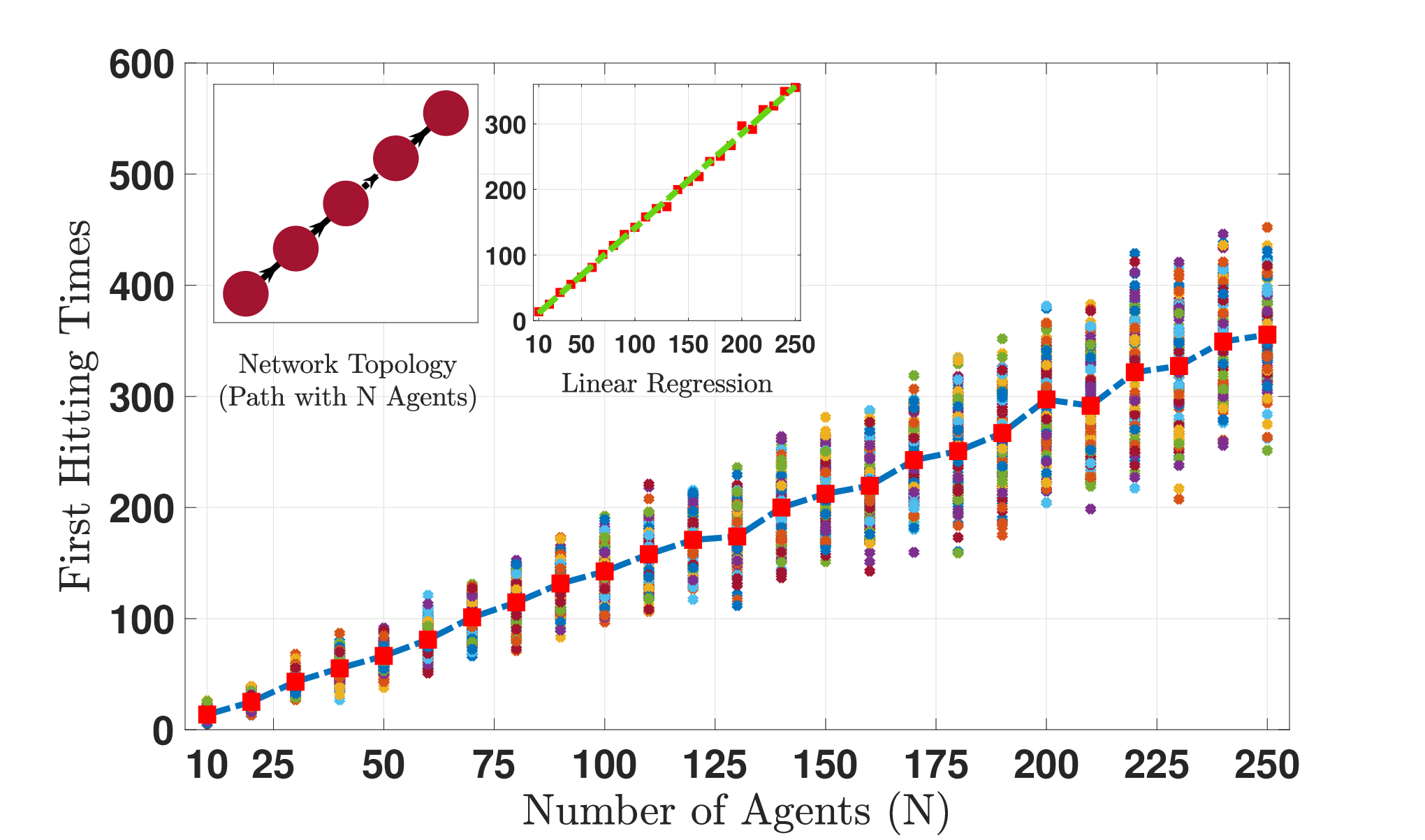
Furthermore, we investigate the dependence of the first hitting time on the size of network. We simulate the SHDS on three different classes of network topologies: complete digraphs, cycle digraphs, and path digraphs. For each class, we vary the number of agents from to , with increments of . The parameters are again chosen uniformly randomly from and the probability of drawing an edge is . For each case (with a fixed class and a fixed size ), we generate initial conditions uniformly randomly from and simulate the SHDS (38). For each sample path, we record the first hitting time . Figures 8, 9, and 10 plot the data for complete-, cycle-, and path-digraphs, respectively. For each figure, the horizontal axis is the network size and the vertical axis is the first hitting time . For each , the crosses represent the first hitting times of the sample paths. There are of them and the red square is the mean. For complete digraphs, the mean decays to a steady state. The variance seems to decay as well. However, this is not the case for cycles or paths. In either case, the average and the variance increase as grows. Using linear regression, we find that the fitting curves for cycles and paths are and , respectively.


6 Conclusions
In this paper we have presented several new results in the context of synchronization of pulse-coupled oscillators evolving over sparse directed graphs. We have shown that robust global fixed-time synchronization can be achieved in quasi-acyclic digraphs using resetting algorithm, and we have characterized scalable tuning guidelines of order that induce this property, which can be selected to achieve acceleration in the synchronization time. We have also established an impossibility result that shows that having a rooted digraph is not sufficient for global synchronization of PCOs. However, by using suitable random communication graphs, we showed that synchronization with probability one can be established for rooted digraphs. Since all our PCOs are modeled by well-posed hybrid systems, our synchronization results are robust with respect to unmodeled dynamics and small bounded disturbances on the states. Future directions will study the development of similar distributed coordination algorithms for more general smooth compact manifolds.
References
- [1] Bryce Beverlin, James Kakalios, Duane Q. Nykamp, and Theoden I. Netoff. Dynamical changes in neurons during seizures determine tonic to clonic shift. Journal of Computational Neuroscience, 33:41–51, 2011.
- [2] F. Bullo. Lectures on Network Systems. Kindle Direct Publishing, 1.3 edition, 2019. With contributions by J. Cortes, F. Dorfler, and S. Martinez.
- [3] Xudong Chen, Mohamed-Ali Belabbas, and Tamer Başar. Controllability of formations over directed time-varying graphs. IEEE Transactions on Control of Network Systems, 4(3):407–416, 2017.
- [4] Florian Dörfler and Francesco Bullo. Synchronization in complex networks of phase oscillators: A survey. Automatica, 50(6):1539–1564, 2014.
- [5] R. Goebel, R. G. Sanfelice, and A. R. Teel. Hybrid dynamical systems. Princeton University Press, NJ, 2012.
- [6] R. L. Graham, M. Grötschel, and L. Lovász, editors. Handbook of Combinatorics (Vol. 1). MIT Press, Cambridge, MA, USA, 1995.
- [7] M. Hartman, A. Subbaraman, and A. R. Teel. Robust global almost sure synchronization on a circle via stochastic hybrid control. In Danielle C. Tarraf, editor, Control of Cyber-Physical Systems, volume 449 of Lecture Notes in Control and Information Sciences, pages 3–21. Springer, 2013.
- [8] J.B. Buck. Synchronous rhythmic flashing of fireflies. The Quarterly Review of Biology, pages 301–314, 1938.
- [9] Deepti Kannapan and Francesco Bullo. Synchronization in pulse-coupled oscillators with delayed excitatory/inhibitory coupling. SIAM J. Control and Optimization, 54:1872–1894, 2016.
- [10] C. M. Kellet and A. R. Teel. Smooth lyapunov functions and robustness of stability for difference inclusions. Systems & Control Letters, 52:395–405, 2004.
- [11] J. Klinglmayr, C. Bettstetter, M. Timme, and C. Kirst. Convergence of self-organizing pulse-coupled oscillator synchronization in dynamic networks. IEEE Transactions on Automatic Control, 62(4):1606–1619, 2017.
- [12] J. Klinglmayr, C. Kirst, C. Bettstetter, and M. Timme. Guaranteeing global synchronization in networks with stochastic interactions. New Journal of Physics, 14(7):073031, jul 2012.
- [13] Y. Kuramoto. Collective synchronization of pulse-coupled oscillators and excitable units. Physica D, 50:15–30, 1991.
- [14] A. Mauroya and R. Sepulchre. Contraction of monotone phase-coupled oscillators. Systems and Control Letters, 61(11):1097–1102, 2012.
- [15] C. G. Mayhew. Hybrid Control for Topologically Constrained Systems, Ph.D Dissertation. University of California, Santa Barbara, 2010.
- [16] R. Mirollo and Steven H. Strogatz. Synchronization of pulse-coupled biological oscillators. 1990.
- [17] Muhammad U. Javed, Jorge I. Poveda, and Xudong Chen. Global synchronization of clocks in directed rooted acyclic graphs: A hybrid systems approach. 2019 IEEE 58th Conference on Decision and Control (CDC), pages 7352–7357.
- [18] J. Nishimura and E. J. Friedman. Robust convergence in pulse-coupled oscillators with delays. Physical review letters, 106(19):1606–1619, 2011.
- [19] J. Nishimura and E. J. Friedman. Probabilistic convergence guarantees for type-II pulse-coupled oscillators. Physical Review E, 86(2):1606–1619, 2012.
- [20] J. D. Nishimura. Designing Pulse Coupled Oscillators to Synchronize. Ph.D. Dissertation, Cornell University, 2013.
- [21] F. Nunez, Y. Wang, and F. J. Doyle. Synchronization of pulse-coupled oscillators on (strongly) connected graphs. IEEE Transactions on Automatic Control, 60(6):1710–1715, 2015.
- [22] F. Nunez, Y. Wang, and F. J. Doyle III. Global synchronization of pulse-coupled oscillators interacting on cycle graphs. Automatica, 52:202–209, 02015.
- [23] F. Nunez, Y. Wang, A.R. Teel, and F. J. Doyle III. Synchronization of pulse-coupled oscillators to a global pacemaker. Systems & Control Letters, 88:75–80, 2016.
- [24] R. Pagliari and A. Scaglione. Scalable network synchronization with pulse-coupled oscillators. IEEE Transactions on Mobile Computing, 10(3):392–405, March 2011.
- [25] C.S. Peskin. Mathematical aspects of heart physiology. Institute of Mathematical Sciences, New York University, 1975.
- [26] S. Phillips, R. Sanfelice, and R. S. Erwin. On the synchronization of two impulsive oscillators under communication constraints. in Proc. of American Control Conference, pages 2443–2448, 2012.
- [27] J. I. Poveda and A. R. Teel. Hybrid mechanisms for robust synchronization and coordination of multi-agent networked sampled-data systems. Automatica, 99:41–53, 2019.
- [28] Jorge I. Poveda and Andrew R. Teel. Hybrid online learning control in networked multiagent systems: A survey. International Journal of Adaptive Control and Signal Processing, 33:228–261, 2019.
- [29] A. V. Proskurnikov and M. Cao. Synchronization of pulse-coupled oscillators and clocks under minimal connectivity assumptions. IEEE Transactions on Automatic and Control, 62:5873–5879, 2017.
- [30] R. Tyrrell Rockafellar and J-B Wets Roger. Variational Analysis. Springer-Verlag, 1998.
- [31] R. G. Sanfelice, R. Goebel, and A. R. Teel. Invariance principles for hybrid systems with connections to detectability and asymptotic stability. IEEE Trans. Autom. Control, 52:2282–2297, 2007.
- [32] A. Sarlette and R. Sepulchre. Consensus optimization on manifolds. SIAM Journal on Control and Optimization, 48(1):56–76, 2009.
- [33] R. Sepulchre, D. A. Paley, and N. E. Leonard. Stabilization of planar collective motion: All-to-all communication. IEEE Transactions on Automatic Control, 52(5):811–824, May 2007.
- [34] E. Sontag. Stability and stabilization: Discontinuities and the effect of disturbances. In Nonlinear Analysis, Differential Equations and Control, volume 528 of NATO Science Series, pages 551–598. 1999.
- [35] E. D. Sontag. Clocks and insensitivity to small measurement errors. ESAIM: Control, Optimisation and Calculus of Variations, 4(4):537–557, 1999.
- [36] A. Subbaraman and A. R. Teel. Recurrence principles and their application to stability theory for a class of stochastic hybrid systems. IEEE Transactions on Automatic Control, 61(11):3477–3492, 2016.
- [37] A. R. Teel and J. I. Poveda. A hybrid systems approach to global synchronization and coordination of multi-agent sampled-data systems. In Proc. of Analysis and Design of Hybrid Systems, pages 123–128, 2015.
- [38] Andrew R. Teel. Lyapunov conditions certifying stability and recurrence for a class of stochastic hybrid systems. Annual Reviews in Control, 37(1):1 – 24, 2013.
- [39] Andrew R. Teel, Anantharaman Subbaraman, and Antonino Sferlazza. Stability analysis for stochastic hybrid systems: A survey. Automatica, 50:2435–2456, 2014.
- [40] Marc Timme, Theo Geisel, and Fred Wolf. Speed of synchronization in complex networks of neural oscillators: Analytic results based on random matrix theory. Chaos: An Interdisciplinary Journal of Nonlinear Science, 16(1), 2006.
- [41] Alexander Tyrrell. Decentralized slot synchronization for cellular mobile radio. 2009.
- [42] H. Wang, W. Yu, W. Ren, and J. Lu. Distributed adaptive finite-time consensus for second-order multiagent systems with mismatched disturbances under directed networks. IEEE Transactions on Cybernetics, 10.1109/TCYB.2019.2903218, pages 1–12, 2019.
- [43] Y. Wang and F. J. Doyle III. Optimal phase response functions for fast pulse-coupled synchronization in wireless sensor networks. IEEE Transactions on Signal Processing, 60(10):5583–5588, Oct 2012.
- [44] Y. Wang, F. Nunez, and F. J. Doyle. Energy-efficient pulse-coupled synchronization strategy design for wireless sensor networks through reduced idle listening. IEEE Transactions on Signal Processing, 60(10):5293–5306, Oct 2012.
- [45] Y. Wang, F. Núñez, and F. J. Doyle. Increasing sync rate of pulse-coupled oscillators via phase response function design: Theory and application to wireless networks. IEEE Transactions on Control Systems Technology, 21(4):1455–1462, July 2013.
Appendix A Notation and Definitions
A set-valued mapping is said to be outer semi-continuous (OSC) at if for all sequences and such that we have that . A set-valued mapping is said to be locally bounded (LB) at if there exists a neighborhood of such that is bounded. Given a set , the mapping is OSC and LB relative to if the set-valued mapping from to defined by for , and by for , is OSC and LB at each . The graph of a set-valued mapping is defined as . Given a set , we use to denote its closure. The outer semi-continuous hull of is the unique set-valued mapping satisfying [30, pp. 155]. Given a measurable space , a set-valued mapping is said to be -measurable [30, Def. 14.1], if for each open set , the set . A sequence of mappings is said to converge graphically if the sequence of sets converges in the sense of set convergence [5, Def. 5.1].
Appendix B Hybrid Dynamical Systems
In this paper we model the dynamics of the network of pulse coupled oscillators using the formalism of hybrid dynamical systems [5]. These systems are modeled by the equations
| (46a) | ||||
| (46b) | ||||
where is the state of the system, is the flow map, which describes the continuous-time dynamics of the state; is called the flow set and it describes the points in the space where is allowed to evolve according to the differential equation (46a); is the jump map and it characterizes the discrete-time dynamics of ; and is called the jump set and it describes the points in the space where is allowed to evolve according to the set-valued update (46). The HDS is represented as . In this paper we restrict our attention to HDS that satisfy the basic conditions of Definition 1. A standard solution to (46) is parameterized by a continuous-time index and a discrete-time index . In particular, solutions to (46) are defined on hybrid time domains. A compact hybrid time domain is a subset of of the form for some and real numbers . A hybrid time domain is a set such that for each , the set is a compact hybrid time domain. A function is said to be a hybrid arc if is a hybrid time domain, and for each such that the interval has non-empty interior the function is locally absolutely continuous. A hybrid arc is said to be a solution to a HDS (46) satisfying the basic conditions if: (1) . (2) If with , then for almost every and . (3) If , then and . A solution to (46) is said to be: a) non-trivial if contains at least two points; b) maximal if there does not exist another solution to such that is a proper subset of and for all ; c) complete if its domain is unbounded; d) eventually discrete if and contains at least two points. d) uniformly non-Zeno if there exists such that for every , if then .
Appendix C Stochastic Hybrid Dynamical Systems
When the jump map in (46b) also depends on a random input , the HDS (46) becomes a stochastic hybrid dynamical system (SHDS) [36] of the form
| (47a) | ||||
| (47b) | ||||
where is a place holder for a sequence of independent, identically distributed i.i.d. input random variables , , defined on a probability space . Thus, for all , and is defined as . We restrict our attention to SHDS that satisfy the basic conditions of Definition 1. Random solutions to SHDS (47) are functions of denoted , such that: 1) has measurability properties that are adapted to the minimal filtration of ; 2) for each the sample path is a standard solution to the HDS (46) with the appropriate dependence on the random input through the jumps. To formally define these mappings, for , let denote the collection of sets , , which are the sub--fields of that form the minimal filtration of , which is the smallest -algebra on that contains the pre-images of -measurable subsets on for times up to . A stochastic hybrid arc is a mapping from to the set of hybrid arcs, such that the set-valued mapping from to , given by , is -measurable with closed-values. Let . An adapted stochastic hybrid arc is a stochastic hybrid arc such that the mapping is measurable for each . An adapted stochastic hybrid arc is a solution to (47) starting from denoted if (with ): (1) ; (2) if with , then for all , and ; (3) if , then and . A random solution is said to be: a) almost surely complete if for almost every sample path the hybrid arc has an unbounded time domain; and almost surely eventually discrete if for almost every sample path the hybrid arc is eventually discrete.
A continuous function is a Lyapunov function relative to a compact set for the SHDS (47) if , is radially unbounded and satisfies , and , where denotes the set of solutions of (47a) with initial condition . The following stochastic hybrid invariance principle, corresponding to [36, Thm. 8], is instrumental in the analysis of SHDS of the form (47).
Theorem 1.
Let be a Lyapunov function relative to a compact set for the SHDS system . Then, is UGASp if and only if there does not exist an almost surely complete solution that remains in a non-zero level set of the Lyapunov function almost surely.
Umar Javed received in 2017 his B.S. degree in Electrical Engineering with minors in Computer Science (AI/ML) and Psychology from the Lahore University of Management Sciences, Pakistan. Currently, he is a PhD candidate in the Department of Electrical, Computer and Energy Engineering at the University of Colorado, Boulder, where he completed his MS in Electrical Engineering in 2019. His interests lie in mathematical control theory and its applications
Jorge I. Poveda is an Assistant Professor in the Department of Electrical, Computer, and Energy Engineering at the University of Colorado, Boulder. He received the M.Sc. and Ph.D. degrees in Electrical and Computer Engineering from the University of California at Santa Barbara in 2016 and 2018, respectively, where he was awarded the Center for Control Dynamical Systems and Computation Outstanding Scholar Fellowship. Before joining CU Boulder, he was a Postdoctoral Fellow at Harvard University in 2018, and a research intern at the Mitsubishi Electric Research Laboratories in 2016 and 2017. In 2020 he received the NSF Career Research Initiation Award (CRII). His research interests lie in the design and analysis of high-performance feedback-based control and optimization algorithms for cyber-physical systems.
Xudong Chen is an Assistant Professor in the Department of Electrical, Computer and Energy Engineering at the University of Colorado, Boulder. Before that, he was a postdoctoral fellow in the Coordinated Science Laboratory at the University of Illinois, Urbana-Champaign. He obtained the B.S. degree from Tsinghua University, Beijing, China, in 2009, and the Ph.D. degree in Electrical Engineering from Harvard University, Cambridge, Massachusetts, in 2014, under the supervision of Roger Brockett. His research interests are in the area of control theory, stochastic processes, optimization, game theory and their applications in modeling, control, and estimation of networked systems and ensemble systems. His research group develops novel engineering methods and advanced mathematical tools for investigating large-scale multi-agent systems. Dr. Chen is an awardee of the 2020 Air Force’s Young Investigator Research Program (YIP).