Quanta Burst Photography502Journal: TOGVolume: 394797DOI: 10.1145/3386569.3392470CCS: Computing methodologies Computational photography

Abstract.
Single-photon avalanche diodes (SPADs) are an emerging sensor technology capable of detecting individual incident photons, and capturing their time-of-arrival with high timing precision. While these sensors were limited to single-pixel or low-resolution devices in the past, recently, large (up to 1 MPixel) SPAD arrays have been developed. These single-photon cameras (SPCs) are capable of capturing high-speed sequences of binary single-photon images with no read noise. We present quanta burst photography, a computational photography technique that leverages SPCs as passive imaging devices for photography in challenging conditions, including ultra low-light and fast motion. Inspired by recent success of conventional burst photography, we design algorithms that align and merge binary sequences captured by SPCs into intensity images with minimal motion blur and artifacts, high signal-to-noise ratio (SNR), and high dynamic range. We theoretically analyze the SNR and dynamic range of quanta burst photography, and identify the imaging regimes where it provides significant benefits. We demonstrate, via a recently developed SPAD array, that the proposed method is able to generate high-quality images for scenes with challenging lighting, complex geometries, high dynamic range and moving objects. With the ongoing development of SPAD arrays, we envision quanta burst photography finding applications in both consumer and scientific photography.
Keywords:
Single-photon camera, single-photon avalanche diode, quanta image sensor, burst photography, super-resolution, high dynamic range, high-speed imaging, low-light imaging1. The Single-Photon Revolution
A conventional camera typically captures hundreds to thousands of photons per pixel to create an image. An emerging class of sensors, called single-photon avalanche diodes (SPADs) (Rochas 2003; Niclass et al. 2005), can record individual photons, and precisely measure their time-of-arrival. Due to their sensitivity and picosecond time resolution, SPADs are driving an imaging revolution. A new generation of devices is emerging, with novel functionalities such as imaging at trillion fps (O’Toole et al. 2017), non-line-of-sight (NLOS) imaging (Buttafava et al. 2015; O’Toole et al. 2018), and microscopic imaging of nano time-scale bio-phenomena (Bruschini et al. 2019).
Passive single-photon imaging:
So far, most SPAD-based imaging systems are active, where the SPAD is used in precise temporal synchronization with an active light source (e.g., a pulsed laser). This includes applications such as NLOS imaging, LiDAR (Shin et al. 2016), and microscopy. Can SPADs be used not just with controlled and precisely synchronized active light sources as is the norm, but more generally under passive, uncontrolled illumination (e.g., sunlight, moonlight)? Such passive SPAD-based imaging systems have the potential to expand the scope of SPADs to a considerably larger set of applications, including machine vision and photography.
Consider a SPAD sensor (an array of SPAD pixels) imaging a scene illuminated by passive lighting. Since photons arrive at the sensor randomly according to Poisson statistics, photon detection events are also random, and can be visualized as a spatio-temporal photon-cube (Fossum 2011). A SPAD camera can capture a sequence of thin, temporal slices of the photon-cube, where each slice is a binary (1-bit) image, as shown in in Fig. 1. Each pixel location records a if it receives one or more photons during the temporal extent of the slice, and otherwise. For example, a recent SPAD camera (Ulku et al. 2019) can capture binary frames per second, at 1/4 MPixel resolution.11 1 Photon-cubes and single-photon binary image sequences were first considered in the context of jots (Fossum 2005; Fossum 2011), another emerging single-photon sensing technology. In this paper, we primarily focus on SPADs due to their high frame rate. However, since both jots and SPADs have similar imaging model and data format, the analysis and techniques presented here are applicable to jots as well. Due to the random nature of photon arrivals, the binary images are stochastic.
Passive single-photon imaging under motion:
How does motion manifest in a stochastic binary image sequence? If the scene (or camera) moves during acquisition, the photons emitted by a scene point get mis-aligned and spread over multiple SPC pixels. In this paper, we propose quanta burst photography, a computational photography technique that computationally re-aligns the photons along motion trajectories, for achieving high-quality images in challenging scenarios, including low-light and high-speed motion (Fig. 1). We develop algorithms that align the binary slices, thus creating a high-bit-depth, high-dynamic-range, potentially super-resolved (via sub-pixel alignment (Park et al. 2003; Wronski et al. 2019)) image of the scene, while minimizing noise and motion blur. This is similar in spirit to conventional burst photography where a burst of noisy, short-exposure images are aligned and merged into a single high-quality image (Hasinoff et al. 2016; Liba et al. 2019). Quanta burst photography can be considered a limiting case because each binary image captures at most one photon per pixel, and is thus extremely noisy and quantized (1-bit). On the other hand, due to fast capture, we have a long sequence available ( frames, depending on light level, dynamic range and motion), instead of as in conventional burst photography.
Why quanta burst photography?
One of the key benefits of SPCs is the low read noise in the raw binary frames (Bruschini et al. 2019), which enables dividing the exposure time finely into a long sequence of frames to handle fast motion. This results in virtually negligible intra-frame motion blur and low noise, even for rapid motion (e.g., sports and wildlife photography). 22 2 For conventional cameras, there is a fixed read noise penalty for each captured frame. Therefore, dividing the exposure time finely into a large number of frames increases the effective read noise in the merged image. Furthermore, although at first glance it may appear that SPCs, due to their high sensitivity, are useful only in photon-starved scenarios, surprisingly, they can also image bright scenes where conventional sensors saturate (Ingle et al. 2019; Antolovic et al. 2018). This is because although each binary image is quantized, a large collection of single-photon measurements, when combined, naturally avoids saturation (Yang et al. 2012), and thus, achieve extreme dynamic range. There are two catalysts for key quanta burst photography:
(a) Emergence of large SPCs arrays:
Till recently, SPCs were available as single-pixel or small arrays (e.g., 32x32 pixels), which, while sufficient for several scientific imaging applications, are not suitable for consumer domain photography. Fortunately, due to their compatibility with mainstream CMOS fabrication lines, it is now possible to develop large SPCs arrays, with the world’s first 1 MPixel jots (Ma et al. 2017) and SPAD arrays (Morimoto et al. 2020) reported recently, while maintaining high sensor quality and room temperature operation.
(b) High-performance burst photography:
We are inspired by the recent success of burst photography algorithms (Hasinoff et al. 2016; Wronski et al. 2019; Liba et al. 2019), which, for the first time, are starting to produce reliably artifact-free images in almost all circumstances, including challenging scenes with occlusions and non-rigid motion. These motion estimation and merging methods are robust enough to be shipped to consumer devices, a gold-standard for computational photography techniques.
We adopt the design principles and best practices from these burst photography approaches, and design algorithms tailored for single-photon binary stochastic images. We demonstrate, via simulations and experiments on a 1/8 megapixel SPAD array (SwissSPAD2 (Ulku et al. 2019)) that quanta burst photography is able to generate high SNR, blur-free and super-resolved images in extreme scenarios (low-light, fast motion, large dynamic range) which would be considered challenging for burst photography on conventional cameras.
Scope and limitations:
Are single-photon cameras and quanta burst photography ready to be deployed on consumer devices? Not yet. So far, we have focused on achieving high image quality. Our current unoptimized implementation, however, is not directly amenable to consumer devices, which have strong constraints on speed, power and memory. The current sensor prototype does not have a color filter array (e.g., a Bayer pattern), and thus, the resulting images are gray-scale. The resolution, although highest to-date among SPAD cameras, is still relatively low (1/8 MPixel) for consumer applications. Fortunately, the capabilities of single-photon sensors continue to improve, with higher resolution (Morimoto et al. 2020) and color sensors (Elgendy and Chan 2019) on the horizon.
The proposed approach is not meant to directly compete with conventional CMOS sensors and burst photography pipelines, which have been optimized over several years, and can produce compelling photographic experiences. Instead, our goal is to explore and analyze a nascent but promising imaging modality, which, if successful, could lead to capabilities (high quality photography in ultra low-light and fast motion) that were hitherto considered impossible. This paper should be seen just as a first step toward that goal.
2. Related Work
Image denoising.
Single image denoising algorithms denoise images by imposing various image prior such as spatial smoothness (Beck and Teboulle 2009), sparsity (Elad and Aharon 2006) and self-similarity (Buades et al. 2005). Such priors are also used in transform domains such as frequency domain (Gonzalez and Woods 2006), wavelets (Malfait and Roose 1997), and 3D transform (BM3D) (Dabov et al. 2007b). Recent data-driven denoising algorithms attempt to capture the noise statistics using a neural network instead of an explicit prior (Zhang et al. 2018b). Single image denoising approaches tend to fail when the image has a very low SNR due to low light, and/or limited exposure time because of fast scene/camera motion. In these cases it is essential to combine information from multiple images to generate a high-quality image.
Burst denoising.
Burst denoising methods take a sequence of underexposed images and merge them into a single image. The SNR is improved since more photons are collected. The key technical challenge for burst denoising is to accurately align and merge frames as the camera moves. This can be addressed either by a two-step align-and-merge approach (Wronski et al. 2019; Liba et al. 2019; Hasinoff et al. 2016; Liu et al. 2014; Heide et al. 2014), or joint optimization (Heide et al. 2016). Recently, deep learning based methods have also been proposed (Godard et al. 2018; Mildenhall et al. 2018). A related problem is video denoising, where both input and output are sequence of images (Chen et al. 2019; Maggioni et al. 2012; Dabov et al. 2007a). Our goal is to create a single, high-quality image from a burst of binary single-photon frames.
Quanta (single-photon) sensors.
Currently, there are two main enabling technologies for large single-photon camera arrays: SPADs and jots. SPADs achieve single photon sensitivity by amplifying the weak signal from each incident photon via avalanche multiplication, which enables zero read noise and extremely high frame rate (kfps). Jots, on the other hand, amplify the single-photon signal by using an active pixel with high conversion gain (low capacitance) (Fossum 2005). By avoiding avalanche, jots achieve smaller pixel pitch, higher quantum efficiency and lower dark current, but have lower temporal resolution (Ma et al. 2017). Although the techniques in this paper are applicable to both SPADs and jots, we primarily focus on SPADs because of their capability to resolve fast motion due to high temporal resolution. We show simulation-based comparisons between the two types of sensors, and a discussion on their relative merits, in Sec. 7.
Wide-dynamic-range sensors.
There are several wide-dynamic-range image sensors based on different technologies, such as logarithmic response (Kavadias et al. 2000) and light-to-frequency conversion (Wang et al. 2006). Such sensors have an extended dynamic range compared to conventional CMOS sensors, but the blur-noise trade-off still exists, which makes them less effective for low-light, fast-motion scenarios. In addition, especially for logarithmic sensors, photo response non-uniformity (PRNU) is a limitation in conventional implementations (Yang et al. 2009); this effect compounds the above issues, significantly limiting image quality.
Image reconstruction from single-photon sensor data.
There is prior work on reconstructing intensity images from single-photon binary frames using denoising techniques such as total variation and BM3D (Chan et al. 2016; Gnanasambandam et al. 2019), or by an end-to-end neural network (Choi et al. 2018; Chandramouli et al. 2019). In the presence of motion, Fossum (Fossum 2013) suggested shifting the binary images to compensate for motion and achieve blur-free image reconstruction. This idea has been implemented recently (Iwabuchi et al. 2019; Gyongy et al. 2018; Gyongy et al. 2017), albeit for simplistic motion models (e.g., planar objects with in-plane motion and no occlusions). Our approach is based on a much less restrictive assumption (motion can be approximated by patch-wise 2D translation and remains constant within temporal blocks), and can reliably produce high-quality images for a broad range of complex, real-world scenes.
3. Passive Single-Photon Imaging Model
Consider a SPC pixel array observing a scene. The number of photons arriving at pixel during an exposure time of seconds is modeled as a Poisson random variable (Yang et al. 2012):
| (1) |
where is the photon flux (photons/seconds) incident at . is the quantum efficiency. Each pixel detects at most one photon during an exposure time, returning a binary value such that if ; otherwise. Due to the randomness in photon arrival, is a random variable with Bernoulli distribution:
| (2) | ||||
where is the dark count rate (DCR), which is the rate of spurious counts unrelated to photons.
To estimate the number of incident photons (proportional to the linear intensity image of the scene), suppose the camera captures a sequence of binary frames. Assuming no motion between binary frames, or that the binary frames are aligned perfectly to compensate for motion, we define as the sum of all binary frames:
| (3) |
where is the binary frame at time , and is the number of frames. is the total number of photons detected at over the entire binary image sequence. Since each binary frame is independent, the expected value of the sum image is the product of the number of frames , and the expected value of the Bernoulli variable :
| (4) |
The maximum likelihood estimate (MLE) of the intensity image is given as (Antolovic et al. 2016):
| (5) |
Dynamic range:
Eq. 4 describes the relationship between , the total number of photons detected by the camera, and , the number of photons incident on the camera (the quantity we wish to estimate). This non-linear relationship (Sbaiz et al. 2009), as plotted in Fig. 2, is similar to the D-log H curve for photographic films proposed by Hurter and Diffield in 1890, because single-photon cameras emulate the silver halide emulsion film process (Fossum 2005). The key observation is that this response curve asymptotically approaches its maximum value (), while never reaching it. This soft saturation (Ingle et al. 2019) suggests that the value of keeps increasing (albeit progressively slowly) as the number of incident photons increases, which means the incident flux can be recovered even for bright scenes. In contrast, the response curve for conventional sensors is a straight line before hitting the full well capacity, and then flattens due to saturation. Therefore, a passive single-photon camera, while capable of imaging low-light scenes, somewhat counter-intuitively, can also image bright scenes where conventional sensors saturate, providing an extremely wide dynamic range.
Read noise:
Conventional sensors convert discrete incident photons to analog current, which is again converted to a discrete number by an analog-to-digital converter (ADC). This discrete analog discrete pipeline results in read noise, which is the dominant source of noise in low-light. This places a limit on exposure time used in conventional burst photography. Given a fixed total capture time, increasing the number of frames may reduce motion artifacts, but since each additional frames incurs a read noise penalty, the SNR of the merged image is lowered. Jots have a deep sub-electron read noise (currently 0.2e- (Ma et al. 2017)), which although considerably lower than conventional CMOS sensors, can still limit the image quality in ultra low-light conditions (Fossum et al. 2016).
In contrast, SPADs directly measure the photon counts, skipping the intermediate analog conversion, thereby avoiding read noise. This allows a SPAD camera to finely divide the exposure time into a large number of binary frames for motion compensation, thereby simultaneously achieving low motion-blur and high SNR.
4. Single-Photon Imaging Under Motion
If the scene or camera moves during capture, then simply summing the binary sequence (Eq. 3) leads to merging of photons from different scene points, resulting in motion blur. Therefore, to avoid motion blur, the binary frames must be aligned to compensate for inter-frame motion before merging them.
Aligning the binary frames directly is challenging because the traditional brightness constancy assumption does not hold for the observed random binary signal due to extremely low SNR. Although it may be possible to estimate the inter-frame motion when the motion is a global, low-dimensional transform such as global 2D translation or global homography, for general, unstructured scenes with unknown geometry, the transform must be formulated as a pixelwise 2D motion field (or optical flow). In this case, the total number of unknown parameters to estimate is for image resolution . Such a complex, high-dimensional motion model cannot be solved precisely from the random binary input data.
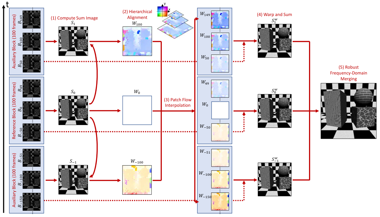
Fortunately, SPADs are able to capture binary frames at high frame rates (97.7kfps for SwissSPAD2 (Ulku et al. 2019)). At such high frame rates, the velocity at each pixel can be treated as a constant within a local temporal window. We use this observation as an additional constraint to solve the otherwise challenging optical flow problem on stochastic binary frames. One way to incorporate such a constraint is to compute a temporally coherent optical flow (Black 1994; Weickert and Schnörr 2001; Volz et al. 2011). In practice, we choose a simple, less computationally intensive approach: We divide the entire image sequence into non-overlapping temporal blocks, compute the sum image for each block (called block-sum images) and align the block-sum images. The block-sum images have a higher SNR than individual binary frames, which makes it possible to use traditional optical flow methods to align them.
Block-level vs. frame-level alignment.
Fig. 3 shows an overview of the method. We call the block in the center of the sequence the reference block. All the other blocks, called auxiliary blocks, are aligned to the reference block. After aligning the block-sum images, we do not use the coarse-temporal-scale motion field between temporal blocks to merge them directly. Instead, we linearly interpolate the motion field in time to obtain motion between successive binary frames. This fine-scale motion field is used to warp each binary frame and align to a central reference frame in the reference block, before merging. This hierarchical approach removes the motion blur within each temporal block, resulting in sharp images even for fast moving scenes. After warping, a frequency-space merging algorithm is used to merge the temporal blocks, which provides robustness to small alignment error. In the next two sections, we provide details of the align and merge algorithms.
5. Aligning Temporal Blocks
Given a reference and an auxiliary block, we compute the 2D correspondence map between them based on their appearance. Instead of using a pixel-wise optical flow algorithm, we use a patch-based alignment approach 33 3 In this paper, we refer to temporal sum of frames as “blocks” and spatial windows of pixels as “patches”. since it is more resilient to noise than pixel-wise optical flow (Bruhn et al. 2005; Zimmer et al. 2011). Furthermore, even for merging (Sec. 6), patch-based approaches achieve more robust results than pixel-based merging (Liu et al. 2014) in low SNR images. For patch-based merging, it is sufficient to compute a motion field at the patch level, thereby saving computational time.
Hierarchical patch alignment.
We use a hierarchical patch alignment approach similar to (Hasinoff et al. 2016) on an image pyramid built from the block-sum images. The number of pyramid levels can be adjusted according to the spatial resolution of the binary images. We use a 3-level pyramid for the 512x256 images used in our experiments. The matching is done by minimizing L1 matching error in a spatial neighborhood. For a patch with indices , which expands the pixel indices , we find the smallest motion vector that minimizes:
| (6) |
The size of the patch is . is the auxiliary block-sum image and is the reference block-sum image.
Spatial regularization at finest level.
We perform a global regularization at the finest level of the pyramid to further refine the patch alignment results (especially for blocks with extremely small number of photons) and to provide sub-pixel alignment for super-resolution. This is performed by minimizing the following energy:
| (7) |
where is the spatial domain for the patch indices . are the motion fields defined on , and is the spatial resolution of the input images. is the matching error defined in Eq. 6. In practice, we minimize the Charbonnier loss as an differentiable alternative for the L1 loss.
Interpolating the motion field.
The computed inter-block motion is treated as motion between the center frames of each block. A linear interpolation is then performed to compute the motion between individual frames. Higher-order interpolation (e.g., cubic or spline) may improve the temporal smoothness, but will increase the dependency on other blocks. In practice, linear interpolation achieves good results for SPADs with high temporal resolution. Fig. 4 shows an example demonstrating the benefits of frame-level interpolation. While alignment at the block level does not remove the motion blur completely, blur is considerably reduced by frame-level interpolation. An evaluation of frame-level interpolation on real data is provided in the supplementary report.

6. Merging Binary Sequence
After estimating inter-frame motion, one way to merge the binary image sequence is to warp the binary images, compute the sum image of all warped images, and finally, compute the MLE of the sum (Eq. 5). However, the estimated motion field may have errors due to occlusions, motion discontinuities, and non-rigid scene deformations. In this case, simply summing the warped binary images will create strong blurring or ghosting artifacts.
Can robust merging be used for binary frames?
Robust merging methods such as Wiener frequency-domain filtering have long been used in video denoising and burst denoising (Hasinoff et al. 2016) to account for potentially incorrect estimated motion. The key idea is that if a patch in a warped frame is significantly different from that in the reference frame, then the alignment is likely erroneous. The final merged patch is computed by taking a weighted average of all matched patches, where the patches with large difference with the reference path (likely erroneous) are given a lower weight. This approach, while successful for conventional cameras, cannot be directly applied to merge the single-photon binary frames. This is because even if two binary frames are perfectly aligned, the difference between the frames could still be high due to the dominating shot noise. As a result, every auxiliary frame will have a low weight, and will make a low contribution to the final merged image, resulting in low SNR, as shown in Fig. 5.
In order to address this limitation, we adopt a two-step approach. First, we warp the frames within each block to the block’s reference frame by using the estimated fine-scale inter-frame motion. The frames are simply added to form a warped block-sum image without any robust merge, since the amount of motion within each block is small, reducing the likelihood of alignment errors. This warping makes it possible to remove the motion blur within each block, as shown in Fig. 4. The warped block-sum images have sufficient SNR to be amenable to a traditional frequency-domain robust-merging approach (Hasinoff et al. 2016). Therefore, Wiener filtering is applied to the warped block-sum images in the second step, so that they can be merged stably to reduce the noise level. Fig. 5 shows the result of applying block-level Wiener filtering, resulting in considerably higher SNR than naive frame-level merging.


Merging with super-resolution:
The high-speed single-photon data leads to small inter-frame motion ( pixels), which can be leveraged to generate a merged image that has a higher resolution than the input frames (Park et al. 2003; Wronski et al. 2019). We develop a simple super-resolution algorithm based on kernel regression by adapting the original merging method described above. As above, after the inter-frame motion field is computed, frames within the same block are warped and added up to form the warped block-sum images. However, instead of computing the weighted average of patches, the weighted patches are treated as a bag of sample points, as shown in Fig. 6. Each patch is warped to sub-pixel locations on a higher-resolution output pixel grid. The algorithm then scans through each pixel on the output grid. At each pixel, an anisotropic Gaussian kernel (Takeda et al. 2007; Wronski et al. 2019) is used to combine the sample points within a spatial neighborhood. Instead of the point-wise robustness term used in recent conventional burst photography (Wronski et al. 2019), our super-resolution method uses the frequency-domain robust merging approach (the same approach used in original-resolution merging). This approach is more robust in practice, at the cost of slightly higher computational complexity. Please refer to the supplementary technical report for design details of the kernel regression method.
Post-denoising and tone mapping:
After using the proposed motion-compensating temporal denoising method to generate a final sum image, existing single-photon image reconstruction methods can be applied for further denoising (see the supplementary report for comparisons of different reconstruction methods). We apply Anscombe transform (Anscombe 1948) to the sum image and apply BM3D (Dabov et al. 2007b) for spatial denoising (Chan et al. 2016).
After merging and denoising, we use Eq. 5 to invert the non-linear response to get a linear image. Gamma correction and tone-mapping is then applied to generate images suited for viewing.


7. Results
7.1. Simulation Results
| Sensor Type | Conventional | Jot | SPAD | ||
|---|---|---|---|---|---|
| Resolution | Same | ||||
| Pixel Pitch | Same | ||||
| Bit Depth | 10 | 1 | 1 | ||
| QE / PDE (R) | 59% | 64% | 17% | ||
| QE / PDE (G) | 64% | 71% | 23% | ||
| QE / PDE (B) | 47% | 62% | 21% | ||
| Read Noise (per pixel) | 2.4 | 0.24 | 0 | ||
|
1/s | 0.16/s | 7.5cps | ||
We simulate the imaging process for a SPAD camera and a conventional camera of the same resolution and pixel pitch. We first simulate the ground-truth linear intensity images using a ray tracer (POV-Ray) and then draw Bernoulli samples according to Eq. 2 to synthesize the binary images. Tab. 1 shows the sensor parameters we used for the simulation. The parameters for the conventional sensor are for a high-end machine-vision camera 44 4 https://www.flir.com/products/grasshopper3-usb3/?model=GS3-U3-123S6C-C. The parameters for the SPAD camera are based on the SwissSPAD2 sensor we use for our experiments. Currently SwissSPAD2 does not have a Bayer filter for color imaging. We do not simulate the Bayer filter and demosaicing process but render the RGB channels directly. The alignment is performed on a grayscale version of the image and the merging is applied to the three channels independently. The fraction of incident photons that are measured by a SPAD is given by its photon detection efficiency (PDE), which is defined as the product of quantum efficiency, fill factor and photon detection probability (PDP). (See Sec. 9 for a detailed discussion.) The PDE used in the simulation is computed by multiplying the PDP of SwissSPAD2 with the spectral response of a set of contrived color filters and the fill factor (assumed to be 50% which can be achieved with microlenses (Antolović et al. 2019)). The dark count rate is assumed to be spatially uniform (no hot pixels). For real images, this non-uniformity can be calibrated and compensated as shown in Eq. 5.
Comparison of conventional and quanta burst photography.
We compare the results for single-shot conventional image, conventional burst photography and quanta burst photography for different lighting conditions. For conventional burst result, we use an approach similar to conventional burst photography methods (Hasinoff et al. 2016). The exposure time and number of bursts are determined using the strategy described in Sec. 8.
Fig. 7 shows the simulation results for different lighting conditions. The scene is kept static while the camera is moving. The trajectory of the camera is set to be a linear 3D translation plus a small, smooth random 6 degrees-of-freedom (DoF) perturbation at each frame. For a scene with sufficient light, both burst methods generate high-quality images. In low light, SPAD-based quanta burst photography generates much better result as there is no read noise. Please refer to the supplementary report for a comparison of the two methods for different motion speeds under extremely low light.
Performance for different types of camera motion.
Fig. 8 shows the quanta burst reconstruction results for different kinds of camera motion, including rotation around y-axis, rotation around z-axis, translation along z-axis and random 6DoF motion. In all cases, relatively blur-free images are reconstructed.
7.2. Comparison between Jots and SPADs
The quanta burst photography approach discussed so far is applicable to both single-photon sensing technologies: SPAD and jots. What are the relative benefits of the two technologies? In this section, we address this question by comparing their performance in various imaging scenarios.
Adapting proposed approaches to spatially oversampling jots.
Due to the spatially oversampling nature of jots, the spatial resolution of raw jots images is typically higher than the final output image (oversampling factor (Yang et al. 2012)). A box filter is applied to downsample the raw binary images (related to the boxcar function used in (Chan et al. 2016)) and convert them to floating point intensity values. The float images are then divided into temporal blocks as with SPADs (although with smaller block sizes than SPADs) and processed through the align and merge pipeline.
Comparison under different amounts of motion.
Fig. 9 shows a comparison between the reconstruction results of SPADs and jots. We simulate two sequences of the same scene where the camera moves at different speeds. Since jots-based devices have yet to achieve a very high resolution (10241024 so far), and their temporal resolution is lower than SPAD (1kHz vs 97.7kHz), we compare SPADs with a “projected jot device” with a resolution of , such that total number of pixel measurements (data bandwidth) of the two sensors is the same. We assign the same data bandwidth to the two sensors based on the assumption that the bandwidth will be an important limiting factor for the frame rate for both sensors, as their specifications evolve in the future.
Under fast motion, the merged image from jots contains motion blur, while SPADs are able to register the binary images and merge them into a sharp image. On the other hand, when the motion is slow, jots are able to generate a sharper image due to their high spatial resolution. Therefore, we envision these two technologies to complement each other: SPADs achieve higher performance in high-speed scenarios, while jots with projected high resolution will achieve better image quality for scenes with relatively slow motion and high-frequency texture details. The reader is referred to the supplementary technical report for more comparisons including those for multi-bit jots, and for comparisons using the sensor parameters of currently available state-of-the-art prototypes for jots (Gnanasambandam et al. 2019) and SPADs (Ulku et al. 2019).


7.3. Experiments
We use a SwissSPAD2 camera (Ulku et al. 2019) to perform real experiments (Fig. 10). This SPAD camera can capture binary frames at a spatial resolution of 512256. The maximum frame rate of the camera is 96.8kHz. The camera does not have microlenses and has a native fill factor of about 13%. Currently the sensor is not equipped with Bayer filters, so only grayscale images are reconstructed. We identify the hot pixels by taking 100000 frames while covering the sensor completely from light sources. The hot pixels are corrected for each binary frame. See the supplementary report for details.
Performance for different lighting conditions.
Fig. 11 shows the performance of quanta burst photography for different lighting conditions. We choose the same still scene for all sequences. The camera was moved horizontally to emsure the motion is controllable and reproducible across different sequences. The conventional camera images are emulated from the captured binary images by first reconstructing the intensity using Eq. 5 and then adding the read noise and quantization error according to the parameters in Tab. 1. Quanta burst photography generates images with higher quality than conventional single and burst images. Even in very low light, where the individual binary frames are sufficiently sparse to make it nearly impossible to make out the scene structure, a reasonable image is reconstructed by aligning and merging the sparse and noisy binary frames. Please see the supplementary report for performance of the proposed method for different camera moving speeds.
The purpose of this experiment is not to compare a conventional sensor and SPAD sensor directly. In fact, due to the low resolution and low quantum efficiency of current SPAD sensors, the SPAD will almost always generate worse-quality images than a commercial CMOS sensor. Here we simulate the conventional images by assuming a conventional sensor with the same resolution and quantum efficiency as the SPAD array. Due to the blur-noise trade-off, conventional sensor struggles in reconstructing high-quality images, while SPAD has the potential of super-sampling in time and mitigate motion blur even for low-light and fast-moving scenes.
Reconstructing challenging scenes.
Fig. 12 shows various scenes involving large depth variations, specular high lights, complex geometry and fine structures. Such scenes are usually challenging for optical flow and block matching algorithms. The camera was handheld, and underwent a random 6DoF motion when capturing the images. Since a long-focus lens is used, even natural hand tremor causes a large apparent motion in the image space. Despite these challenges, the proposed method is able to reconstruct blur-free images with high SNR.
Comparison of denoising algorithms.
After aligning and merging the binary frames into a sum image with low noise and blur, its SNR can be further improved via spatial denoising algorithms (e.g., BM3D (Dabov et al. 2007b), total variation (TV) (Chan and Lu 2014)). BM3D is applied as a post-processing step after the Anscombe transform, whereas total variation is formulated as a joint reconstruction and denoising optimization problem (Chan and Lu 2014). Fig. 13 compares the results of different combinations of spatio-temporal denoising schemes. Traditional single-photon image reconstruction (naive average) contains either motion blur in the long sequence, or heavy noise in the short sequence which cannot be perfectly removed using BM3D. In contrast, quanta burst photography approach in combination with spatial denoising is able to generate sharp, less noisy image. In our experiments, BM3D consistently performs better than TV, which results in over-smoothing for short exposure, and loss of contrast for long exposure. See the supplementary technical report for more comparisons.
Super-resolution.
Fig. 14 demonstrates the performance of the super-resolution algorithm. A high-resolution lens is used with the camera which creates aliasing in the image when the scene is perfectly in focus. The super-resolution algorithm is able to utilize the aliasing and sub-pixel motion between frames to create a higher-resolution image with sharper image details and less aliasing artifacts than the normal merging algorithm.
Reconstructing high dynamic range scenes.
Fig. 15 shows a high dynamic range scene captured by the SPAD array. The only light source in the scene, the lamp (red box), is directly visible in the image, which is about 2000 times brighter than the text on the plaque (blue box), which does not receive any direct light. Similar as in Fig. 11, we simulate the conventional images by adding read noise and quantization error. With a single capture, the conventional image is either saturated around the lamp, or cannot recover the texts on the plaque. Conventional burst photography improves the dynamic range, but the text is still indiscernible due to read noise. Quanta burst photography is able to recover both the filament and the text at the same time.

Resolving scene motion.
Since the proposed method only computes patch-wise motion and does not assume any global motion model, it is capable of resolving scene motion. Fig. 16 shows a person plucking the lowest two strings on the guitar. Simple averaging of binary frames creates ghosting artifacts or strong noise. Our method is able to resolve the plucking motion of the thumb and the vibration of the strings with lower noise.
Indoor scenes with different, natural lighting.
In addition to the controlled scenes in the lab, we captured a few indoor scenes with more natural lighting. As shown in Fig. 17, the proposed method is able to reconstruct high-quality images under these unstructured environments. Please refer to the supplementary technical report for more simulation and experimental results.
8. When to Use Quanta Burst Photography?
What are the imaging regimes where quanta burst photography can outperform conventional cameras? 55 5 This analysis is not meant to be a direct comparison between current single-photon and conventional cameras. Conventional CMOS sensors have considerably higher spatial resolution and color filters, and thus, will achieve better image quality as compared to current SPAD arrays in the foreseeable future. The goal of this analysis is to provide guidelines on when using quanta burst photography can be beneficial, assuming SPAD arrays can match the spatial resolution of sCMOS sensors. To address this question, we characterize the performance of conventional and quanta burst photography in terms of the SNR of the reconstructed linear image:
| (8) |
where is the estimated image intensity, and is the root mean squared error of the estimate. We assume that the input images are perfectly aligned (no mis-alignment errors) for both conventional and single-photon cameras, so that the estimation error is only due to image noise.
Conventional cameras:
The image formation of conventional image sensors is given by an affine model (Hasinoff et al. 2010):
| (9) |
where is the photon counts as in Eq. 1 ( and are the exposure time and quantum efficiency for the conventional sensor). is the read noise. is the dark current noise caused by thermal current with flux . These three components are statistically independent of each other. To simplify the analysis, we assume all images are captured at the same ISO speed and temperature such that and are fixed.
Suppose a conventional burst photography algorithm captures a burst of images. The process of merging the captured images into a result image can be viewed as a maximum likelihood estimation process. Assuming the images are perfectly aligned such that the images can be merged simply by taking their average:
| (10) |
where is the image captured at time . We assume the dark current noise can be calibrated at each pixel. The mean of the calibrated dark current noise is subtracted from the sum of images to give an unbiased estimate of the photon flux (linear intensity image).
From the noise model, the root mean squared error (RMSE) of this estimator due to noise variance is given by
| (11) |
where is the total exposure time for the sequence.
SPAD cameras:
A maximum likelihood estimator for SPAD camera is derived in Eq. 5. For a sufficiently long sequence , the variance of the MLE can be estimated using Fisher information (See the supplementary technical report for the derivation):
| (12) |
where and are the exposure time and quantum efficiency for the single-photon camera.
The RMSE for both modalities depend on the total exposure time of the image sequence (assumed same for both modalities for a fair comparison) and the total number of frames and , which, in practice, in turn depend on the photon flux level and camera motion: longer exposure is preferred when the light level is low and the camera is moving slowly. (Liba et al. 2019) proposes “motion metering” which automatically selects the exposure time based on a prediction of future scene and camera motion. We take a similar approach for our analysis: we assume the scene and camera motion are known or can be estimated such that and can be determined according to the following three principles: (1) When the motion is slow, the total exposure time is chosen to meet a target total number of photons to ensure high SNR. (2) When the motion is fast, the total exposure time is limited by a maximum amount of motion across the sequence. (3) The total number of frames is chosen to ensure the per-frame motion blur is below a threshold. Details about the strategy can be found in the supplementary report. The SNR of both approaches can then be expressed as a function of photon flux and camera motion, which allows comparison of the two approaches.
SNR comparisons between conventional and SPAD cameras:
Fig. 18 plots the difference of SNRs () in dB for a wide range of photon fluxes and apparent speeds. Fig. 18 (a) compares the burst photography performance between a current SPAD sensor and a machine-vision CMOS sensor with parameters listed in Tab. 1. At ultra low light and high speeds, the SPAD sensor performs considerably better than the CMOS sensor (up to 27.5dB = 23.7 times). On the other hand, in well-lit scenes with negligible motion, the SPAD performs worse (albeit at most by a factor of ) due to relatively low PDE and high DCR of current SPAD arrays.
Recently, advanced CMOS sensors used in high-end cellphones have achieved sub-electron read noise. Fig. 18 (b) plots the SNR difference between current SPADs and iPhone 7’s sensor, which is reported to have a read noise of 0.68 electrons (Claff [n.d.]). Such low read noise makes its performance better than current SPADs for a wider range of flux intensity and motion speeds. Since SPADs are an emerging technology, their specifications (in particular, resolution and PDE) continue to improve, arguably at a faster rate than conventional sensors which are already a mature technology. Fig. Supp18 (c) compares iPhone 7’s sensor with a projected SPADs which achieve a PDE of 50%. To visualize the variations of the SNR difference with respect to one specific parameter, we show 1-D slices of the comparison between iPhone 7 and current/projected SPAD sensor in (d) and (e), where either the photon flux or the apparent speed is fixed. These figures demonstrate how the proposed analysis framework can be used to direct future development of SPADs for best performance under certain light levels and amount of motion. A theoretical dynamic range analysis can be found in the supplementary technical report.
9. Outlook on Single-Photon Sensors
In this section, we discuss the current state and future outlook of SPAD sensor arrays, in terms of their key characteristics: spatial resolution, temporal frame rate, photon detection efficiency (PDE), and the dark count rate (DCR).
Spatial resolution:
Due to their compatibility with mainstream CMOS fabrication lines, it was predicted in 2008 that SPAD image sensors could reach large resolutions within one decade (Charbon 2007; Charbon 2008). In recent years, significant effort has been devoted to achieve this goal, with the world’s first 1 MPixel SPAD array reported recently (Morimoto et al. 2020). With the same fabrication process, it is possible to go up to 5-10 MPixel, not far from their counterparts in CMOS imagers in several cell-phone cameras. Can we go even higher (e.g., 50 MPixel) in the long term? The key factor that limits the spatial resolution is the minimum pixel pitch, which in turn is limited by the necessity of placing a guard ring 66 6 A SPAD pixel detects single photons by creating an avalanche of photo-electrons (large current) when a photon is incident, and sensing the avalanche current via a comparator or a high-gain amplifier. A guard ring is a region around each SPAD pixel that forces the avalanche to be confined in the region, in order to prevent edge breakdown. Guard rings are implemented via geometric structures that are not sensitive to light. around each SPAD pixel. In current CMOS technologies, due to the guard ring, SPAD pitch cannot be reduced below m. At that pitch, the guard ring occupies a large portion of the pixel, thus reducing the fill factor to a minimum. This limitation could be addressed via 3D-stacking (Pavia et al. 2015), a potentially effective way to reduce SPAD pixel pitch by moving all the active and passive components associated with a SPAD pixel to the bottom tier of the sensor.
Frame rate and power consumption:
The frame rate of a SPAD sensor array is limited by the bit-rate the chip can deliver and by the number of communication channels it can host. For example, a 1 Mpixel camera with a frame rate of 1kfps, will generate 1Gbps of data, which can be handled by a single LVDS (low-voltage differential signalling) communication channel. Typically, this kind of channel requires about 10mW of power at full speed. If one wants to increase the frame rate by, say, , then the data rate will increase to 100Gbps, with W of power required, which may be prohibitive for consumer devices. This assumes that the internal power dissipation due to SPADs and chip operation is negligible, and that the readout speed of the pixels internally is not the bottleneck. The communication power consumption can be mitigated by performing on-chip image processing operations, and designing more efficient motion computation and image alignment operations that are amenable to on-chip processing. Furthermore, it is possible to exploit the spatio-temporal sparsity in the photon-cube raw data in low-light scenarios. Depending on the light-level in the scene, one could achieve a considerable data rate reduction by compressing the raw photon-cube data (Zhang et al. 2018a).
Photon detection efficiency (PDE):
PDE is defined as the product of the pixel fill factor, and the photon detection probability (PDP), which is the probability that an impinging photon generates a detectable signal. PDP is the product of quantum efficiency and the probability of triggering an avalanche. PDP is dependent on the wavelength of photons; for current devices, the PDP is typically at nm. Due to low fill factors, earlier SPAD arrays had PDEs as low as making them highly inefficient due to significant light loss. However, the PDE in recent arrays has increased to approximately by using microlens arrays, which increase PDE by effectively increasing the fill factor. While still lagging the quantum efficiency of conventional sensors (approximately ), the PDE of SPAD arrays will likely improve due to improving fabrication processes, including 3D stacking.
Dark count rate (DCR):
DCR is the rate of avalanche counts unrelated to photons, measured in counts-per-second (cps). Earlier SPAD devices were largely considered impractical due to high DCR, up to several tens of cps at cryogenic temperatures, and tens of kcps at room temperature. Fortunately, for current devices, DCR has been drastically reduced to cps (Morimoto et al. 2020), even at room temperature. Since SPADs do not have read noise, this DCR is sufficiently low to achieve nearly shot-noise-limited SNR, even in ultra low-light. Since DCR is proportional to the active area of a SPAD, as the pixels become smaller, DCR could be further reduced.
10. Limitations and Discussion
Resolving larger range of motions.
The proposed alignment algorithm assumes the motion of the spatial image patches can be approximated by a 2D translation, which is usually appropriate for camera motion and rigid object motion. When this assumption does not hold, the discrepancies between the true deformation of the patch and the translation approximation can be mitigated by the robust merging algorithm. However, when the scene contains several small objects or undergoes nonrigid motion, such an approximation no longer holds, which can result in artifacts in the merged image. An interesting future research direction is to design optical flow algorithms for aligning images for such challenging scenes.
Fast, energy-efficient processing.
Currently, our algorithms are implemented in unoptimized MATLAB code which takes about 30 minutes for processing a sequence with 10000 binary frames, which is far from real-time. For consumer photography applications, it is critical to perform the processing in a fast and also energy-efficient way. In our current implementation, the binary frames are treated as real numbers (e.g., when warping them during the merging stage). One potential way to improve the efficiency is to utilize specialized computing architectures and algorithms for binary data (Daruwalla et al. 2019; Pfeiffer and Pfeil 2018).
Bandwidth limitation.
The high dynamic range of SPADs comes at the cost of large bandwidth requirement. Currently, the captured binary images are stored on-board, and then transferred to a PC and processed offline. The bandwidth requirement can be relaxed by capturing multi-bit images (which sacrifices temporal resolution). The bandwidth in future SPAD sensors can also be improved by using faster interfaces such as PCIexpress and CameraLink.
Video reconstruction.
The proposed method can be used for reconstructing videos by shifting the reference frame in time. An example reconstructed video for the guitar sequence is shown in the supplementary video. While the current approach reconstructs the video sequence one frame at a time, novel algorithms that enforce temporal coherency across reconstructed frames could be developed, resulting in improved video quality as well as lower computational complexity.
Free-running SPADs.
The proposed techniques are designed for SPAD arrays operating in synchronous clock-driven mode where all the pixels read off measurements simultaneously, at fixed intervals. It has recently been shown that event-driven (Antolovic et al. 2018) or free-running SPADs (Ingle et al. 2019) achieve a higher dynamic range by recharging the SPAD as soon as the dead time due to a photon detection is over. An interesting future direction is to design quanta burst photography techniques for asynchronous SPAD arrays where pixels return binary measurement independently.
Quanta image processing pipeline.
The primary focus of this paper is on the alignment and merging of binary images. We apply denoising and tone-mapping as a post-processing step to the merged images. For modern camera systems with color filter arrays, there are several other essential processing steps in the image processing pipeline including demosaicking, white balancing, and dehazing. Specifically, demosaicking is a non-trivial problem since temporal interpolation of alignment can introduce color artifacts. Recent research suggests that there is a potential benefit of performing end-to-end processing from the raw sensor data (Heide et al. 2014; Gharbi et al. 2016; Chen et al. 2019). A promising next step is to design a similar framework for quanta burst photography and explore whether similar benefits exist for single-photon images.
Acknowledgements.
This research is supported in part by the Sponsor DARPA REVEAL program , a Sponsor Wisconsin Alumni Research Foundation (WARF) Fall Competition award (UW-Madison), the Sponsor Swiss National Science Foundation Grant Grant #166289 and Sponsor The Netherlands Organization for Scientific Research Project Grant #13916 (EPFL).References
- (1)
- Anscombe (1948) F J Anscombe. 1948. The Transformation of Poisson, Binomial and Negative-Binomial Data. Biometrika 35, 3/4 (1948), 246–254.
- Antolovic et al. (2018) Ivan Michel Antolovic, Claudio Bruschini, and Edoardo Charbon. 2018. Dynamic Range Extension for Photon Counting Arrays. Optics Express 26, 17 (Aug. 2018), 22234.
- Antolovic et al. (2016) Ivan Michel Antolovic, Samuel Burri, Claudio Bruschini, Ron Hoebe, and Edoardo Charbon. 2016. Nonuniformity Analysis of a 65-Kpixel CMOS SPAD Imager. IEEE Transactions on Electron Devices 63, 1 (Jan. 2016), 57–64.
- Antolović et al. (2019) Ivan Michel Antolović, Arin Can Ulku, Ekin Kizilkan, Scott Lindner, Frédéric Zanella, Rolando Ferrini, Marc Schnieper, Edoardo Charbon, and Claudio Bruschini. 2019. Optical-Stack Optimization for Improved SPAD Photon Detection Efficiency. In Quantum Sensing and Nano Electronics and Photonics XVI, Manijeh Razeghi, Jay S. Lewis, Giti A. Khodaparast, and Eric Tournié (Eds.). SPIE, San Francisco, United States, 99.
- Ashikhmin (2002) Michael Ashikhmin. 2002. A Tone Mapping Algorithm for High Contrast Images. In Eurographics Workshop on Rendering. 145–156.
- Beck and Teboulle (2009) A. Beck and M. Teboulle. 2009. Fast Gradient-Based Algorithms for Constrained Total Variation Image Denoising and Deblurring Problems. IEEE Transactions on Image Processing 18, 11 (Nov. 2009), 2419–2434.
- Black (1994) Michael J. Black. 1994. Recursive Non-Linear Estimation of Discontinuous Flow Fields. In European Conference on Computer Vision (ECCV), Gerhard Goos, Juris Hartmanis, and Jan-Olof Eklundh (Eds.), Vol. 800. Springer Berlin Heidelberg, Berlin, Heidelberg, 138–145.
- Bruhn et al. (2005) Andrés Bruhn, Joachim Weickert, and Christoph Schnörr. 2005. Lucas/Kanade Meets Horn/Schunck: Combining Local and Global Optic Flow Methods. International Journal of Computer Vision (IJCV) 61, 3 (2005), 211–231.
- Bruschini et al. (2019) Claudio Bruschini, Harald Homulle, Ivan Michel Antolovic, Samuel Burri, and Edoardo Charbon. 2019. Single-Photon Avalanche Diode Imagers in Biophotonics: Review and Outlook. Light: Science & Applications 8, 1 (Dec. 2019), 87.
- Buades et al. (2005) A. Buades, B. Coll, and J.-M. Morel. 2005. A Non-Local Algorithm for Image Denoising. In IEEE Computer Society Conference on Computer Vision and Pattern Recognition (CVPR), Vol. 2. IEEE, San Diego, CA, USA, 60–65.
- Buttafava et al. (2015) Mauro Buttafava, Jessica Zeman, Alberto Tosi, Kevin Eliceiri, and Andreas Velten. 2015. Non-line-of-sight imaging using a time-gated single photon avalanche diode. Optics express 23, 16 (2015), 20997–21011.
- Chan et al. (2016) Stanley Chan, Omar Elgendy, and Xiran Wang. 2016. Images from Bits: Non-Iterative Image Reconstruction for Quanta Image Sensors. Sensors 16, 11 (Nov. 2016), 1961.
- Chan and Lu (2014) Stanley H. Chan and Yue M. Lu. 2014. Efficient Image Reconstruction for Gigapixel Quantum Image Sensors. In IEEE Global Conference on Signal and Information Processing (GlobalSIP). IEEE, Atlanta, GA, USA, 312–316.
- Chandramouli et al. (2019) Paramanand Chandramouli, Samuel Burri, Claudio Bruschini, Edoardo Charbon, and Andreas Kolb. 2019. A Bit Too Much? High Speed Imaging from Sparse Photon Counts. In IEEE International Conference on Computational Photography (ICCP). Tokyo, Japan, 1–9. arXiv:1811.02396
- Charbon (2007) E. Charbon. 2007. Will Avalanche Photodiode Arrays Ever Reach 1 Megapixel? Image Sensors Workshop (2007).
- Charbon (2008) E. Charbon. 2008. Towards large scale CMOS single-photon detector arrays for lab-on-chip applications. J. of Phys. D: Appl. Phys. 41 (12) (2008).
- Chen et al. (2019) Chen Chen, Qifeng Chen, Minh N Do, and Vladlen Koltun. 2019. Seeing Motion in the Dark. In International Conference on Computer Vision (ICCV). 3185–3194.
- Choi et al. (2018) Joon Hee Choi, Omar A. Elgendy, and Stanley H. Chan. 2018. Image Reconstruction for Quanta Image Sensors Using Deep Neural Networks. In IEEE International Conference on Acoustics, Speech and Signal Processing (ICASSP). IEEE, Calgary, AB, 6543–6547.
- Claff ([n.d.]) William J. Claff. [n.d.]. Input-Referred Read Noise versus ISO Setting. https://www.photonstophotos.net/Charts/RN_e.htm.
- Dabov et al. (2007a) Kostadin Dabov, Alessandro Foi, and Karen Egiazarian. 2007a. Video Denoising by Sparse 3D Transform-Domain Collaborative Filtering. In European Signal Processing Conference. 145–149.
- Dabov et al. (2007b) Kostadin Dabov, Alessandro Foi, Vladimir Katkovnik, and Karen Egiazarian. 2007b. Image Denoising by Sparse 3-D Transform-Domain Collaborative Filtering. IEEE Transactions on Image Processing 16, 8 (Aug. 2007), 2080–2095.
- Daruwalla et al. (2019) Kyle Daruwalla, Heng Zhuo, Carly Schulz, and Mikko Lipasti. 2019. BitBench: A Benchmark for Bitstream Computing. In ACM SIGPLAN/SIGBED International Conference on Languages, Compilers, and Tools for Embedded Systems (LCTES). ACM Press, Phoenix, AZ, USA, 177–187.
- Elad and Aharon (2006) Michael Elad and Michal Aharon. 2006. Image Denoising Via Sparse and Redundant Representations Over Learned Dictionaries. IEEE Transactions on Image Processing 15, 12 (Dec. 2006), 3736–3745.
- Elgendy and Chan (2019) Omar A. Elgendy and Stanley H. Chan. 2019. Color Filter Arrays for Quanta Image Sensors. https://arxiv.org/abs/1903.09823 (2019).
- Fossum (2005) Eric Fossum. 2005. What To Do With Sub-Diffraction Limit (SDL) Pixels?—A Proposal for a Gigapixel Digital Film Sensor (DFS). In IEEE Workshop on Charge-Coupled Devices and Advanced Image Sensors. 214–217.
- Fossum et al. (2016) Eric Fossum, Jiaju Ma, Saleh Masoodian, Leo Anzagira, and Rachel Zizza. 2016. The Quanta Image Sensor: Every Photon Counts. Sensors 16, 8 (Aug. 2016), 1260.
- Fossum (2011) Eric R. Fossum. 2011. The Quanta Image Sensor (QIS): Concepts and Challenges. In OSA Topical Mtg on Computational Optical Sensing and Imaging. Toronto, Canada.
- Fossum (2013) Eric R. Fossum. 2013. Modeling the Performance of Single-Bit and Multi-Bit Quanta Image Sensors. IEEE Journal of the Electron Devices Society 1, 9 (Sept. 2013), 166–174.
- Gharbi et al. (2016) Michaël Gharbi, Gaurav Chaurasia, Sylvain Paris, and Frédo Durand. 2016. Deep Joint Demosaicking and Denoising. ACM Transactions on Graphics 35, 6 (Nov. 2016), 1–12.
- Gnanasambandam et al. (2019) Abhiram Gnanasambandam, Omar Elgendy, Jiaju Ma, and Stanley H. Chan. 2019. Megapixel Photon-Counting Color Imaging Using Quanta Image Sensor. Optics Express 27, 12 (June 2019), 17298.
- Godard et al. (2018) Clément Godard, Kevin Matzen, and Matt Uyttendaele. 2018. Deep Burst Denoising. In European Conference on Computer Vision (ECCV), Vittorio Ferrari, Martial Hebert, Cristian Sminchisescu, and Yair Weiss (Eds.). Springer International Publishing, Cham, 538–554.
- Gonzalez and Woods (2006) Rafael C. Gonzalez and Richard E. Woods. 2006. Digital Image Processing (3rd Edition). Prentice-Hall, Inc., USA.
- Gyongy et al. (2017) Istvan Gyongy, Tarek Al Abbas, Neale A W Dutton, and Robert K Henderson. 2017. Object Tracking and Reconstruction with a Quanta Image Sensor. In International Image Sensor Workshop (IISW). 5.
- Gyongy et al. (2018) Istvan Gyongy, Neale Dutton, and Robert Henderson. 2018. Single-Photon Tracking for High-Speed Vision. Sensors 18, 2 (Jan. 2018), 323.
- Hasinoff et al. (2010) Samuel W. Hasinoff, Frédo Durand, and William T. Freeman. 2010. Noise-Optimal Capture for High Dynamic Range Photography. In IEEE Computer Society Conference on Computer Vision and Pattern Recognition (CVPR). 553–560.
- Hasinoff et al. (2016) Samuel W. Hasinoff, Dillon Sharlet, Ryan Geiss, Andrew Adams, Jonathan T. Barron, Florian Kainz, Jiawen Chen, and Marc Levoy. 2016. Burst Photography for High Dynamic Range and Low-Light Imaging on Mobile Cameras. ACM Transactions on Graphics 35, 6 (Nov. 2016), 1–12.
- Heide et al. (2016) Felix Heide, Steven Diamond, Matthias Nießner, Jonathan Ragan-Kelley, Wolfgang Heidrich, and Gordon Wetzstein. 2016. ProxImaL: Efficient Image Optimization Using Proximal Algorithms. ACM Transactions on Graphics 35, 4 (July 2016), 1–15.
- Heide et al. (2014) Felix Heide, Karen Egiazarian, Jan Kautz, Kari Pulli, Markus Steinberger, Yun-Ta Tsai, Mushfiqur Rouf, Dawid Pająk, Dikpal Reddy, Orazio Gallo, Jing Liu, and Wolfgang Heidrich. 2014. FlexISP: A Flexible Camera Image Processing Framework. ACM Transactions on Graphics 33, 6 (Nov. 2014), 1–13.
- Ingle et al. (2019) Atul Ingle, Andreas Velten, and Mohit Gupta. 2019. High Flux Passive Imaging with Single-Photon Sensors. In IEEE Conference on Computer Vision and Pattern Recognition (CVPR). 6760–6769.
- Iwabuchi et al. (2019) Kiyotaka Iwabuchi, Tomohiro Yamazaki, and Takayuki Hamamoto. 2019. Iterative Image Reconstruction for Quanta Image Sensor by Using Variance-Based Motion Estimation. In International Image Sensor Workshop (IISW). 4.
- Kavadias et al. (2000) S. Kavadias, B. Dierickx, D. Scheffer, A. Alaerts, D. Uwaerts, and J. Bogaerts. 2000. A Logarithmic Response CMOS Image Sensor with On-Chip Calibration. IEEE Journal of Solid-State Circuits 35, 8 (Aug. 2000), 1146–1152.
- Liba et al. (2019) Orly Liba, Ryan Geiss, Samuel W. Hasinoff, Yael Pritch, Marc Levoy, Kiran Murthy, Yun-Ta Tsai, Tim Brooks, Tianfan Xue, Nikhil Karnad, Qiurui He, Jonathan T. Barron, and Dillon Sharlet. 2019. Handheld Mobile Photography in Very Low Light. ACM Transactions on Graphics 38, 6 (Nov. 2019), 1–16.
- Liu et al. (2014) Ziwei Liu, Lu Yuan, Xiaoou Tang, Matt Uyttendaele, and Jian Sun. 2014. Fast Burst Images Denoising. ACM Transactions on Graphics 33, 6 (Nov. 2014), 1–9.
- Ma et al. (2017) Jiaju Ma, Saleh Masoodian, Dakota A. Starkey, and Eric R. Fossum. 2017. Photon-Number-Resolving Megapixel Image Sensor at Room Temperature without Avalanche Gain. Optica 4, 12 (Dec. 2017), 1474.
- Maggioni et al. (2012) Matteo Maggioni, Giacomo Boracchi, Alessandro Foi, and Karen Egiazarian. 2012. Video Denoising, Deblocking, and Enhancement Through Separable 4-D Nonlocal Spatiotemporal Transforms. IEEE Transactions on Image Processing 21, 9 (Sept. 2012), 3952–3966.
- Malfait and Roose (1997) M. Malfait and D. Roose. 1997. Wavelet-Based Image Denoising Using a Markov Random Field a Priori Model. IEEE Transactions on Image Processing 6, 4 (April 1997), 549–565.
- Mildenhall et al. (2018) Ben Mildenhall, Jonathan T. Barron, Jiawen Chen, Dillon Sharlet, Ren Ng, and Robert Carroll. 2018. Burst Denoising with Kernel Prediction Networks. In IEEE/CVF Conference on Computer Vision and Pattern Recognition (CVPR). IEEE, Salt Lake City, UT, 2502–2510.
- Morimoto et al. (2020) Kazuhiro Morimoto, Andrei Ardelean, Ming-Lo Wu, Arin Can Ulku, Ivan Michel Antolovic, Claudio Bruschini, and Edoardo Charbon. 2020. Megapixel time-gated SPAD image sensor for 2D and 3D imaging applications. Optica 7, 4 (Apr 2020), 346–354.
- Niclass et al. (2005) C. Niclass, A. Rochas, P.-A. Besse, and E. Charbon. 2005. Design and Characterization of a CMOS 3-D Image Sensor Based on Single Photon Avalanche Diodes. IEEE Journal of Solid-State Circuits 40, 9 (Sept. 2005), 1847–1854.
- O’Toole et al. (2017) M. O’Toole, F. Heide, D. B. Lindell, K. Zang, S. Diamond, and G. Wetzstein. 2017. Reconstructing Transient Images from Single-Photon Sensors. In 2017 IEEE Conference on Computer Vision and Pattern Recognition (CVPR). 2289–2297.
- O’Toole et al. (2018) Matthew O’Toole, David B. Lindell, and Gordon Wetzstein. 2018. Confocal non-line-of-sight imaging based on the light-cone transform. Nature 555 (Mar 2018), 338–341.
- Park et al. (2003) Sung Cheol Park, Min Kyu Park, and Moon Gi Kang. 2003. Super-Resolution Image Reconstruction: A Technical Overview. IEEE Signal Processing Magazine 20, 3 (May 2003), 21–36.
- Pavia et al. (2015) Juan Mata Pavia, Mario Scandini, Scott Lindner, Martin Wolf, and Edoardo Charbon. 2015. A 1 × 400 Backside-Illuminated SPAD Sensor With 49.7 Ps Resolution, 30 pJ/Sample TDCs Fabricated in 3D CMOS Technology for Near-Infrared Optical Tomography. IEEE Journal of Solid-State Circuits 50, 10 (Oct. 2015), 2406–2418.
- Pfeiffer and Pfeil (2018) Michael Pfeiffer and Thomas Pfeil. 2018. Deep Learning With Spiking Neurons: Opportunities and Challenges. Frontiers in Neuroscience 12 (Oct. 2018), 774.
- Rochas (2003) Alexis Rochas. 2003. Single Photon Avalanche Diodes in CMOS Technology. Ph.D. Dissertation. EPFL.
- Sbaiz et al. (2009) Luciano Sbaiz, Feng Yang, Edoardo Charbon, Sabine Susstrunk, and Martin Vetterli. 2009. The Gigavision Camera. In IEEE International Conference on Acoustics, Speech and Signal Processing (ICASSP). IEEE, Taipei, Taiwan, 1093–1096.
- Shin et al. (2016) Dongeek Shin, Feihu Xu, Dheera Venkatraman, Rudi Lussana, Federica Villa, Franco Zappa, Vivek K. Goyal, Franco N. C. Wong, and Jeffrey H. Shapiro. 2016. Photon-efficient imaging with a single-photon camera. Nature Communications 7 (Jun 2016), 12046.
- Takeda et al. (2007) Hiroyuki Takeda, Sina Farsiu, and Peyman Milanfar. 2007. Kernel Regression for Image Processing and Reconstruction. IEEE Transactions on Image Processing 16, 2 (Feb. 2007), 349–366.
- Ulku et al. (2019) Arin Can Ulku, Claudio Bruschini, Ivan Michel Antolovic, Yung Kuo, Rinat Ankri, Shimon Weiss, Xavier Michalet, and Edoardo Charbon. 2019. A 512 × 512 SPAD Image Sensor With Integrated Gating for Widefield FLIM. IEEE Journal of Selected Topics in Quantum Electronics 25, 1 (Jan. 2019), 1–12.
- Volz et al. (2011) Sebastian Volz, Andres Bruhn, Levi Valgaerts, and Henning Zimmer. 2011. Modeling Temporal Coherence for Optical Flow. In IEEE International Conference on Computer Vision (ICCV). IEEE, Barcelona, Spain, 1116–1123.
- Wang et al. (2006) Xiuling Wang, Winnifred Wong, and Richard Hornsey. 2006. A High Dynamic Range CMOS Image Sensor With Inpixel Light-to-Frequency Conversion. IEEE Transactions on Electron Devices 53, 12 (Dec. 2006), 2988–2992.
- Weickert and Schnörr (2001) Joachim Weickert and Christoph Schnörr. 2001. Variational Optic Flow Computation with a Spatio-Temporal Smoothness Constraint. Journal of Mathematical Imaging and Vision 14, 3 (2001), 245–255.
- Wronski et al. (2019) Bartlomiej Wronski, Ignacio Garcia-Dorado, Manfred Ernst, Damien Kelly, Michael Krainin, Chia-Kai Liang, Marc Levoy, and Peyman Milanfar. 2019. Handheld Multi-Frame Super-Resolution. ACM Transactions on Graphics 38, 4 (July 2019), 1–18. arXiv:1905.03277
- Yang et al. (2012) Feng Yang, Y. M. Lu, L. Sbaiz, and M. Vetterli. 2012. Bits From Photons: Oversampled Image Acquisition Using Binary Poisson Statistics. IEEE Transactions on Image Processing 21, 4 (April 2012), 1421–1436.
- Yang et al. (2009) Feng Yang, Luciano Sbaiz, Edoardo Charbon, Sabine Susstrunk, and Martin Vetterli. 2009. Image Reconstruction in the Gigavision Camera. In IEEE International Conference on Computer Vision Workshops (ICCV Workshops). IEEE, Kyoto, 2212–2219.
- Zhang et al. (2018a) C. Zhang, S. A. Lindner, I. M. Antolovic, J. M. Pavia, M. Wolf, and E. Charbon. 2018a. A 30-frames/s, 252x144 SPAD Flash LiDAR with 1728 Dual-Clock 48.8-ps TDCs, and Pixel-Wise Integrated Histogramming. IEEE Journal of Solid-State Circuits 54 (4) (2018).
- Zhang et al. (2018b) Kai Zhang, Wangmeng Zuo, and Lei Zhang. 2018b. FFDNet: Toward a Fast and Flexible Solution for CNN-Based Image Denoising. IEEE Transactions on Image Processing 27, 9 (Sept. 2018), 4608–4622.
- Zimmer et al. (2011) Henning Zimmer, Andrés Bruhn, and Joachim Weickert. 2011. Optic Flow in Harmony. International Journal of Computer Vision (IJCV) 93, 3 (July 2011), 368–388.