Resource Allocation for Multi-Cell
IRS-Aided NOMA Networks

Inspired by the aforementioned benefits of both IRSs and NOMA, the IRS-aided NOMA transmission scheme can be regarded as an innovative and promising candidate for the next-generation networks. Although some research contributions on IRS-aided NOMA networks have addressed the challenging transmission power and reflection beamforming optimization problem iteratively, the system models are limited to single-cell and/or single-carrier setups [22, 28, 27]. The motivations and challenges of this paper are summarized as follows:

• •

  Currently, there is still a paucity of research contributions on investigating the IRS-aided multi-cell NOMA networks with multiple subchannels, especially for the user association and resource allocation problem with the mutual SIC decoding constraints and individual quality of service (QoS) constraints.

• •

  So far, it is still a challenging issue to maximize the achievable sum rate by jointly designing the transmission power, reflection matrix, and decoding order, while guaranteeing the QoS requirements of all users within the available power budget.

• •

  Moreover, the combinational optimization with respect to ( w.r.t.) the user association and subchannel assignment is NP-hard. The complexity of exhaustive search is exponential, and it is non-trivial to obtain an optimal scheme in the polynomial-time complexity.

In order to tackle the aforementioned challenges, we study the resource allocation problem in IRS-aided multi-cell NOMA networks to maximize the sum rate, especially the interplay between IRS and NOMA. Compared to the single-cell NOMA network in [27] and [28], the decoding order optimization of the multi-cell NOMA networks becomes more complex even without integrating IRSs into the networks. Different from [10] and [20], the highly coupled variables in multi-cell IRS-aided NOMA networks make the signal processing and performance improvement more complicated, e.g., the co-design of decoding order and reflection matrix is investigated in our work. Against the aforementioned background, the main contributions of this paper are summarized as follows:

1. 1.

   We propose a novel framework of resource allocation in the multi-cell NOMA network for enhancing the spectrum efficiency with the aid of a single IRS. We formulate the sum-rate maximization problem subject to the SIC decoding conditions, QoS requirements, and maximum power constraints by jointly optimizing the decoding order, transmission power, reflection matrix, user association, and subchannel assignment. We analyze that the formulated problem is a mixed-integer non-linear programming (MINLP) problem, which is NP-hard and is non-trivial to solve directly.

2. 2.

   In order to tackle the non-linear optimization problem of joint power allocation, reflection matrix design and decoding order determination, we first adopt relaxation methods such as convex upper bound substitution and SCA to transform the non-convex constraints into convex ones, which can be solved by suboptimal solutions with polynomial time complexity. Afterwards, we invoke the semidefinite relaxation (SDP) and Gaussian randomization methods to handle the rank-one constraint. Finally, the decoding order is obtained according to the combined channel gains arranged in ascending order.

3. 3.

   In an effort to solve the three-dimensional (3D) matching problem among users, BSs and subchannels, we first reformulate the decomposed two-dimensional (2D) subproblems into many-to-many (one) matching games that have peer effects but lack substitutability. Then, based on the swap operation, we develop two efficient matching algorithms to achieve a two-sided exchange-stable state among the involved players. Finally, we analyze the stability, convergence, complexity and optimality of the proposed algorithms from a theoretical perspective.

4. 4.

   We demonstrate that the proposed resource allocation algorithms outperform the benchmarks in terms of sum rate and energy efficiency, while NOMA is capable of achieving a better performance than conventional OMA. Additionally, the performance of NOMA networks can be further improved with the aid of the IRS.

The rest of this paper is organized as follows. First, the system model and problem formulation of the IRS-aided multi-cell NOMA network is given in Section II. Then, the sum-rate maximization problem is solved in Section III and IV. Finally, numerical simulations are presented in Section V, which is followed by conclusions in Section VI.

As illustrated in Fig. 1, we consider an IRS-aided multi-cell NOMA transmission scenario¹¹ 1 This paper focuses on the single-antenna case to work on a neat model for providing succinct insights, the algorithms proposed in this paper can be extended to the multi-antenna case as well by exploiting the problem similarity, details of which are omitted here for simplicity., where an IRS is deployed for enhancing wireless service from $J$ single-antenna BSs to $I$ single-antenna cellular users, while $\mathcal{I}=\{1,2,\dots,I\}$ and $\mathcal{J}=\{1,2,\dots,J\}$. It is assumed that each cell is served by one BS, and each cellular user has to be associated with one BS. The IRS is equipped with $M$ passive reflecting elements, denoted by $\mathcal{M}=\{1,2,\dots,M\}$. The diagonal reflection matrix of IRS is denoted by $\mathbf{\Theta}=\text{diag}\left\{\lambda_{1}e^{j\theta_{1}},\lambda_{2}e^{j\theta_{2}},\dots,\lambda_{M}e^{j\theta_{M}}\right\}$, where $\lambda_{m}\in[0,1]$ and $\theta_{m}\in[0,2\pi]$ denote the reflection amplitude²² 2 Without loss of generality, we set $\lambda_{m}=1,\forall m$ to simplify the analysis in the rate-centric communication networks, where the IRS is usually deployed to enhance the amplitude of the reflective signals. and phase shift of the $m$-th element equipped on the IRS, respectively. The total bandwidth $W$ is divided into $K$ subchannels, denoted by $\mathcal{K}=\{1,2,\dots,K\}$, and all subchannels can be reused among BSs to improve the spectrum efficiency. In an effort to reduce the decoding complexity of SIC procedure at the receiver, we assume that the number of paired NOMA users, simultaneously sharing the available spectrum in each cell, is no more than $A_{\text{max}}$, while $A_{\text{max}}\geq 2$. The investigation of more complicated user grouping schemes over subchannels may further enhance the achievable performance of the considered networks at the cost of complexity, but the performance comparison of different user grouping schemes is beyond the scope of this paper. Additionally, it is an interesting and meaningful research topic to adopt a proper user grouping scheme under different scenarios and requirements, which should be included in our future work with the aid of the results derived in this paper.

In the NOMA downlink transmission, let $\alpha_{ij}\in\{0,1\}$ and $\beta_{jk}\in\{0,1\}$ denote the user association indicator and subchannel assignment factor, respectively. Specifically, we have $\alpha_{ij}=1$ if the $i$-th user is associated with the $j$-th BS, otherwise $\alpha_{ij}=0$. Furthermore, we have $\beta_{jk}=1$ if the $k$-th subchannel is assigned to the $j$-th BS, otherwise $\beta_{jk}=0$. Hence, the $i$-th user will be served by the $j$-th BS on the $k$-th subchannel if and only if $\alpha_{ij}\beta_{jk}=1$, otherwise $\alpha_{ij}\beta_{jk}=0$. Then, the superimposed signal, $x_{jk}$, broadcasted by the $j$-th BS on the $k$-th subchannel can be given by

where $x_{ijk}$ and $p_{ijk}$ denote the signal and power transmitted by BS $j$ on subchannel $k$ for user $i$, respectively.

Considering the intra-cell and inter-cell interference on the $k$-th subchannel [29, 30, 35], the received signal of user $i$ associated with BS $j$ on subchannel $k$ is expressed as³³ 3 The channels in this work are considered as frequency-flat fading (or sometimes called quasi-static channels) such as in [21, 22, 23, 24, 26], the effect of multi-path delay is very small and there is no inter-symbol interference. Thus, it is reasonable to ignore the time delay difference between direct and reflective links.

where $h_{ijk}$ denotes the Rayleigh fading channel between BS $j$ and user $i$ on subchannel $k$ [28], $\mathbf{f}_{jk}\in\mathbb{C}^{M\times 1}$ represents Rician fading channels between BS $j$ and IRS on subchannel $k$ [23], $\mathbf{g}_{ik}\in\mathbb{C}^{M\times 1}$ formulates Rayleigh fading channels between IRS and user $i$ on subchannel $k$ [35], and $z_{ijk}$ indicates the additive white Gaussian noise (AWGN) with zero mean and variance $\sigma^{2}$, i.e., $z_{ijk}\sim\mathcal{CN}(0,\sigma^{2})$.

We denote the SIC decoding order as $\pi_{jk}(i)$ for the user $i$ associated with BS $j$ on subchannel $k$. Specifically, we have $\pi_{jk}(i)=n$ if the message of user $i$ is the $n$-th signal to be decoded at the receiver, namely, user $i$ first decodes the signals of all the previous $(n-1)$ users, and then successively subtracts their signals to decode its own desired signal. For example, two users $i$ and $\tilde{i}$ associated with BS $j$ on subchannel $k$, satisfying $\pi_{jk}(i)\leq\pi_{jk}(\tilde{i})$, user $\tilde{i}$ is capable of successfully canceling interference from the superposition signal of user $i$ with the aid of SIC. Let $H_{ijk}=h_{ijk}+\mathbf{g}_{ik}^{H}\mathbf{\Theta}\mathbf{f}_{jk}$ denote the combined channel gain, and $P_{ijk}=\alpha_{ij}\beta_{jk}p_{ijk}$ represents the power allocation. Then, the decoding order constraints for guaranteeing success SIC can be formulated as the equation (3).

where $I_{ijk}^{\text{intra}}=\left|H_{ijk}\right|^{2}\sum_{\pi_{jk}(\hat{i})>\pi_{jk}(i)}P_{\hat{i}jk}$ and $I_{ijk}^{\text{inter}}=\sum_{s=1,s\neq j}^{J}\left|H_{isk}\right|^{2}\sum_{t=1}^{I}P_{tsk}$ are the intra-cell and inter-cell interference, respectively.

It indicates that the achievable SINR of user $\tilde{i}$ to decode user $i$ is no less than that of user $i$. By simple operations, the inequality (3) can be reformulated as the equation (4).

Accordingly, the received SINR of user $i$ associated with BS $j$ on subchannel $k$ is given by

Therefore, the corresponding achievable downlink data rate of user $i$ associated with BS $j$ on subchannel $k$ is calculated as

By jointly designing user association, subchannel assignment, reflection matrix, power allocation, and decoding order in the IRS-aided multi-cell NOMA network, the objective of this paper is to maximize the sum rate of users subject to the SIC decoding constraints, the QoS requirements, and the maximum power constraints, etc. Hence, the optimization problem can be formulated as

where the optimization variables are given in (7a), $R_{\text{min}}$ is the minimum data rate required by each user, $P_{\text{max}}$ is the maximum transmission power provided by each BS, and $\Omega_{jk}$ is the set of all possible SIC decoding orders⁴⁴ 4 For example, if there are three users in set $\Omega_{jk}$, indexed by $i_{1}$, $i_{2}$ and $i_{3}$, then the permutations can be given as $\Omega_{jk}=\{(i_{1},i_{2},i_{3}),(i_{1},i_{3},i_{2}),(i_{2},i_{1},i_{3}),(i_{2},i_{3},i_{1}),(i_{3},i_{1},i_{2}),(i_{3},i_{2},i_{1})\}$. for the users associated with the $j$-th cell on the $k$-th subchannel. Constraint (7c) ensures that the SIC decoding can be conducted successfully at the receiver. Constraint (7d) guarantees that the QoS requirement of each user is satisfied. Constraint (7e) denotes the available transmission power for BSs. Constraint (7f) represents that each user is associated with one BS. Constraint (7g) indicates that the number of users multiplexed in each cell is no less than two, and no more than $A_{\text{max}}$. Constraints (7h)-(7i) describe that each BS is assigned with at least one subchannel, and vice versa. Constraints (7j)-(7m) are invoked for restricting the indication factors, phase shifts, transmit power and decoding order, respectively.

Due to the existence of integer variables $\alpha_{ij}$, $\beta_{jk}$ and the continuous variables $p_{ijk}$, $\mathbf{\Theta}$, as well as their highly coupling at the non-convex objective function and constraints, It can be observed that the sum-rate maximization problem (7) is a MINLP problem, which is NP-hard [14] and is non-trivial to solve optimally by common standard optimization approaches. Additionally, the exhaustive search is not feasible, since the computational complexity grows exponentially over the total number of variables. Therefore, it is essential to transform problem (7) into some tractable convex subproblems, which can be solved separately and alternatively over iterations. To this end, the alternating optimization method can be invoked as an intuitive approach to solve the original MINLP problem (7) in an efficient manner.

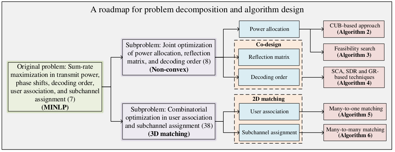
Fig. 2 gives an overview of the roadmap for the proposed problem decomposition and the designed algorithms to the corresponding subproblems. As one can see, the challenging problem (7) is decomposed into a non-convex problem (8) and a combinatorial optimization problem (38), which are efficiently solved by the optimization methods and matching theory in Section III and Section IV, respectively.

For an overview, the designed alternating optimization algorithm for sum-rate maximization in IRS-aided multi-cell NOMA networks is summarized in Algorithm 1. Specifically, the initial points are found by the feasibility-searching algorithm, i.e., Algorithm 3. In the first step, power allocation is performed based on Algorithm 2. In the second step, the co-design of reflection matrix and decoding order is obtained according to Algorithm 4. In the third step, the user association is executed by Algorithm 5. In the fourth step, the subchannel assignment is conducted via Algorithm 6. Then, the above steps are performed alternatively until converge. Accordingly, the complexity and convergence of the four-step Algorithm 1 are provided in the following remark.

Given the reflection matrix and decoding order in problem (9), the power allocation subproblem can be given by

Note that the constraint (7c) can be equivalently expressed as

Since the constraint in (11) is linear w.r.t. power allocation $\mathbf{p}$, it is convex for problem (10) with a given user association and subchannel assignment. At this point, it can be noticed that all constraints in problem (10) are convex excluding the constraint (9d), which is rewritten as

where $\hat{P}_{ijk}=\sum_{\pi_{jk}(\hat{i})>\pi_{jk}(i)}P_{\hat{i}jk}$, $\bar{P}_{ijk}=\sum\limits_{s\neq j}\frac{\left|H_{isk}\right|^{2}}{\left|H_{ijk}\right|^{2}}\sum\nolimits_{t=1}^{I}P_{tsk}$, and $\xi_{ijk}=\frac{\sigma^{2}}{|H_{ijk}|^{2}}$. It is worth noting that the product terms $\gamma_{ijk}\hat{P}_{ijk}$ and $\gamma_{ijk}\bar{P}_{ijk}$ are both non-convex, and thus the SINR constraint in (12) is still not a convex constraint. Therefore, it is necessary to transform the constraint (12) into a convex one.

Let $f(\gamma_{ijk},\hat{P}_{ijk})=\gamma_{ijk}\hat{P}_{ijk}$, while $\gamma_{ijk},\hat{P}_{ijk}\geq 0$. By replacing $f(\gamma_{ijk},\hat{P}_{ijk})$ with its convex upper bound (CUB) [36], the resulting constraint becomes convex⁵⁵ 5 According to the proof of Lemma 1 in [37], the tightness of CUB can be derived similarly, which is thus omitted here for brevity.. To this end, we define the following function

where $\boldsymbol{\lambda}=\{\lambda_{ijk}|\forall i,j,k\}$ is a coefficient set. It can be proved that (13) is a convex function, and $g(\gamma_{ijk},\hat{P}_{ijk},\lambda_{ijk})\geq f(\gamma_{ijk},\hat{P}_{ijk})$ is satisfied for all $\lambda_{ijk}>0$ [28, 36]. Moreover, it can be derived that the equation will turn to equality when $\lambda_{ijk}={\hat{P}_{ijk}}/{\gamma_{ijk}}$. Similarly, let $\bar{f}(\gamma_{ijk},\bar{P}_{ijk})=\gamma_{ijk}\bar{P}_{ijk}$, then its corresponding CUB can be given as

where $\boldsymbol{\bar{\lambda}}=\{\bar{\lambda}_{ijk}|\forall i,j,k\}$ is the coefficient set for $\bar{g}$. Therefore, by replacing $f$ and $\bar{f}$ with (13) and (14), constraint (12) can be transformed into the following convex one.

Next, by replacing (9d) with its approximate constraint (15), it can be observed that both the objective function and all constraints in problem (10) become convex, and hence the Karush-Kuhn-Tucker (KKT) solution of (10) can be iteratively updated until convergence by optimally solving its convex approximation problem with CVX. The details of the proposed CUB-based power allocation algorithm with an adjustable convergence accuracy $\epsilon$ are summarized in Algorithm 2, where the fixed coefficients $\gamma_{ijk}$ and $\bar{\gamma}_{ijk}$ in the $n_{2}$-th iteration can be updated by

Usually, it is non-trivial and difficult to find the initial feasible points $\mathbf{p}^{(0)}$ and $\boldsymbol{\gamma}^{(0)}$ in Algorithm 2. To reduce the sensitivity of Algorithm 2 to the feasibility of the initial points, we formulate a new error minimization problem and propose a novel feasibility-searching algorithm. Let $\bar{\epsilon}\geq 0$ denotes the distance (also called ‘feasibility error’) from the initial points to the feasible domain, then the feasible point search problem can be developed as [28]

where $H=\left|H_{\tilde{i}jk}\right|^{2}\left|H_{isk}\right|^{2}-\left|H_{ijk}\right|^{2}\left|H_{\tilde{i}sk}\right|^{2}$. Note that the substituted problem of (10) and problem (18) have the same set of feasible $\mathbf{p}$ and $\boldsymbol{\gamma}$, while problem (18) is more robust than the former in terms of the initial solution, e.g., it does not request initial points $\mathbf{p}^{(0)}$ and $\boldsymbol{\gamma}^{(0)}$ in the feasible domain. Furthermore, it is worth pointing out that problem (18) is a jointly convex optimization problem, which can be efficiently solved by CVX as well. As a result, the proposed feasibility-searching method is given in Algorithm 3.

With the converged results $\mathbf{p}^{*}$ and $\boldsymbol{\gamma}^{*}$ obtained from Algorithm 2, problem (9) is simplified into the following feasibility-check subproblem

Due to the coupling of $\mathbf{\Theta}$ and $\boldsymbol{\pi}$ in constraint (7c) and the non-convexity of constraint (9d), problem (19) is non-convex and difficult to be solved directly. Alternatively, in order to make this problem tractable, we first consider the problem of reflection matrix design under a determined SIC decoding order, then in turn a low-complexity algorithm for decoding order determination is designed based on the combined channel gain tuned by the IRS.

Specifically, with given $\boldsymbol{\pi}$, the problem (19) is reduced to

where the non-convex constraints in (7c) and (9d) can be equivalently expressed as the following (21) and (22), respectively.

First of all, to handle the non-convexity of constraint (21), we introduce the new variables $a_{\tilde{i}jk}=\left|H_{\tilde{i}jk}\right|^{2}$, $b_{isk}=\left|H_{isk}\right|^{2}$, $c_{ijk}=\left|H_{ijk}\right|^{2}$, and $d_{\tilde{i}sk}=\left|H_{\tilde{i}sk}\right|^{2}$, then constraint (21) can be reformulated as

Then, by adopting an approximation of the difference of two convex functions (DC), the constraint (23) can be approximated by

where the left-hand side is the first-order Taylor expansion of $a_{\tilde{i}jk}b_{isk}$ at the point $(a_{\tilde{i}jk}^{(n)},b_{isk}^{(n)})$ obtained after the $n$-th iteration, and the right-hand side is the first-order Taylor expansion of the non-convex term $c_{ijk}d_{\tilde{i}sk}$ at the point $(c_{ijk}^{(n)},d_{\tilde{i}sk}^{(n)})$, similarly.

Next, to handle the non-convexity of constraint (22), we first define $\boldsymbol{\rho}_{ijk}=\text{diag}\{\mathbf{g}_{ik}^{H}\}\mathbf{f}_{jk}$ and $\boldsymbol{\nu}=[\nu_{1},\nu_{2},\dots,\nu_{M}]^{H}$, where $\nu_{m}=e^{j\theta_{m}}$. Then, we have

References

- [1] W. Ni, X. Liu, Y. Liu et al., “Intelligent reflecting surface aided multi-cell NOMA networks,” in Proc. IEEE Global Commun. Conf. (GLOBECOM) Workshops, Taipei, Taiwan, Dec. 2020, accepted.
- [2] Q. Wu and R. Zhang, “Towards smart and reconfigurable environment: Intelligent reflecting surface aided wireless network,” IEEE Commun. Mag., vol. 58, no. 1, pp. 106–112, Jan. 2020.
- [3] L. Lu, G. Y. Li, A. L. Swindlehurst et al., “An overview of massive MIMO: Benefits and challenges,” IEEE J. Sel. Topics Signal Process., vol. 8, no. 5, pp. 742–758, Oct. 2014.
- [4] W. Roh, J. Seol, J. Park et al., “Millimeter-wave beamforming as an enabling technology for 5G cellular communications: Theoretical feasibility and prototype results,” IEEE Commun. Mag., vol. 52, no. 2, pp. 106–113, Feb. 2014.
- [5] Q. Wu and R. Zhang, “Intelligent reflecting surface enhanced wireless network via joint active and passive beamforming,” IEEE Trans. Wireless Commun., vol. 18, no. 11, pp. 5394–5409, Nov. 2019.
- [6] C. Huang, S. Hu, G. C. Alexandropoulos et al., “Holographic MIMO surfaces for 6G wireless networks: Opportunities, challenges, and trends,” IEEE Wireless Commun., vol. 27, no. 5, pp. 118–125, Oct. 2020.
- [7] Y. Liu, Z. Qin, and Z. Ding, Non-Orthogonal Multiple Access for Massive Connectivity. Switzerland: Springer, 2020.
- [8] Y. Liu, Z. Qin, M. Elkashlan et al., “Nonorthogonal multiple access for 5G and beyond,” Proc. IEEE, vol. 105, no. 12, pp. 2347–2381, Dec. 2017.
- [9] Z. Ding, Y. Liu, J. Choi et al., “Application of non-orthogonal multiple access in LTE and 5G networks,” IEEE Commun. Mag., vol. 55, no. 2, pp. 185–191, Feb. 2017.
- [10] J. Cui, Y. Liu, Z. Ding et al., “QoE-based resource allocation for multi-cell NOMA networks,” IEEE Trans. Wireless Commun., vol. 17, no. 9, pp. 6160–6176, Sept. 2018.
- [11] L. Lei, D. Yuan, C. K. Ho et al., “Power and channel allocation for non-orthogonal multiple access in 5G systems: Tractability and computation,” IEEE Trans. Wireless Commun., vol. 15, no. 12, pp. 8580–8594, Dec. 2016.
- [12] F. Fang, H. Zhang, J. Cheng et al., “Energy-efficient resource allocation for downlink non-orthogonal multiple access network,” IEEE Trans. Commun., vol. 64, no. 9, pp. 3722–3732, Sept. 2016.
- [13] F. Liu and M. Petrova, “Dynamic power allocation for downlink multi-carrier NOMA systems,” IEEE Commun. Lett., vol. 22, no. 9, pp. 1930–1933, Sept. 2018.
- [14] J. Cui, Y. Liu, Z. Ding et al., “Optimal user scheduling and power allocation for millimeter wave NOMA systems,” IEEE Trans. Wireless Commun., vol. 17, no. 3, pp. 1502–1517, Mar. 2018.
- [15] Z. Ding, P. Fan, and H. V. Poor, “Impact of user pairing on 5G nonorthogonal multiple-access downlink transmissions,” IEEE Transa. Veh. Technol., vol. 65, no. 8, pp. 6010–6023, Aug. 2016.
- [16] J. Cui, Z. Ding, and P. Fan, “Outage probability constrained MIMO-NOMA designs under imperfect CSI,” IEEE Trans. Wireless Commun., vol. 17, no. 12, pp. 8239–8255, Dec. 2018.
- [17] L. You, D. Yuan, L. Lei et al., “Resource optimization with load coupling in multi-cell NOMA,” IEEE Trans. Wireless Commun., vol. 17, no. 7, pp. 4735–4749, July 2018.
- [18] Y. Liu, X. Li, F. R. Yu et al., “Grouping and cooperating among access points in user-centric ultra-dense networks with non-orthogonal multiple access,” IEEE J. Sel. Areas Commun., vol. 35, no. 10, pp. 2295–2311, Oct. 2017.
- [19] Y. Fu, Y. Chen, and C. W. Sung, “Distributed power control for the downlink of multi-cell NOMA systems,” IEEE Trans. Wireless Commun., vol. 16, no. 9, pp. 6207–6220, Sept. 2017.
- [20] L. Lei, L. You, Y. Yang et al., “Load coupling and energy optimization in multi-cell and multi-carrier NOMA networks,” IEEE Trans. Veh. Technol., vol. 68, no. 11, pp. 11 323–11 337, Nov. 2019.
- [21] J. Zhao, Y. Liu, K. K. Chai et al., “Spectrum allocation and power control for non-orthogonal multiple access in HetNets,” IEEE Trans. Wireless Commun., vol. 16, no. 9, pp. 5825–5837, Sept. 2017.
- [22] T. Hou, Y. Liu, Z. Song et al., “Reconfigurable intelligent surface aided NOMA networks,” IEEE J. Sel. Areas Commun., 2020, accepted, doi: 10.1109/JSAC.2020.3007039.
- [23] S. Zhang and R. Zhang, “Capacity characterization for intelligent reflecting surface aided MIMO communication,” IEEE J. Sel. Areas.Commun., vol. 38, no. 8, pp. 1823–1838, 2020.
- [24] Y. Cheng, K. H. Li, Y. Liu et al., “Downlink and uplink intelligent reflecting surface aided networks: NOMA and OMA,” May 2020. [Online]. Available: http://arxiv.org/abs/2005.00996
- [25] Z. Ding and H. V. Poor, “A simple design of IRS-NOMA transmission,” IEEE Commun. Lett., vol. 24, no. 5, pp. 1119–1123, May 2020.
- [26] H. Zhang, B. Di, L. Song et al., “Reconfigurable intelligent surfaces assisted communications with limited phase shifts: How many phase shifts are enough?” IEEE Trans. Veh. Technol., vol. 69, no. 4, pp. 4498–4502, Apr. 2020.
- [27] X. Mu, Y. Liu, L. Guo et al., “Capacity and optimal resource allocation for IRS-assisted multi-user communication systems,” Jan. 2020. [Online]. Available: https://arxiv.org/abs/2001.03913
- [28] J. Zuo, Y. Liu, Z. Qin et al., “Resource allocation in intelligent reflecting surface assisted NOMA systems,” IEEE Trans. Commun., 2020, accepted, doi: 10.1109/TCOMM.2020.3016742.
- [29] C. Pan, H. Ren, K. Wang et al., “Multicell MIMO communications relying on intelligent reflecting surfaces,” IEEE Trans. Wireless Commun., vol. 19, no. 8, pp. 5218–5233, Aug. 2020.
- [30] J. Zuo, Y. Liu, E. Basar et al., “Intelligent reflecting surface enhanced millimeter-wave NOMA systems,” IEEE Commun. Lett., 2020, accepted, doi: 10.1109/LCOMM.2020.3009158.
- [31] C. Huang, A. Zappone, G. C. Alexandropoulos et al., “Reconfigurable intelligent surfaces for energy efficiency in wireless communication,” IEEE Trans. Wireless Commun., vol. 18, no. 8, pp. 4157–4170, Aug. 2019.
- [32] X. Liu, Y. Liu, Y. Chen et al., “RIS enhanced massive non-orthogonal multiple access networks: Deployment and passive beamforming design,” IEEE J. Sel. Areas Commun., 2020, accepted, doi: 10.1109/JSAC.2020.3018823.
- [33] Q. Wu and R. Zhang, “Beamforming optimization for wireless network aided by intelligent reflecting surface with discrete phase shifts,” IEEE Trans. Commun., vol. 68, no. 3, pp. 1838–1851, Mar. 2020.
- [34] B. Zheng, Q. Wu, and R. Zhang, “Intelligent reflecting surface-assisted multiple access with user pairing: NOMA or OMA?” IEEE Commun. Lett., vol. 24, no. 4, pp. 753–757, Apr. 2020.
- [35] H. Xie, J. Xu, and Y. Liu, “Max-min fairness in IRS-aided multi-cell MISO systems via joint transmit and reflective beamforming,” Feb. 2020. [Online]. Available: http://arxiv.org/abs/1912.12827
- [36] L. Tran, M. F. Hanif, A. Tolli et al., “Fast converging algorithm for weighted sum rate maximization in multicell MISO downlink,” IEEE Signal Process. Lett., vol. 19, no. 12, pp. 872–875, Dec. 2012.
- [37] X. Xie, F. Fang, and Z. Ding, “Joint optimization of beamforming, phase-shifting and power allocation in a multi-cluster IRS-NOMA network,” Sept. 2020. [Online]. Available: https://arxiv.org/abs/2009.06233