Resilient Consensus Against
Mobile Malicious Agents
Abstract
This paper addresses novel consensus problems in the presence of adversaries that can move within the network and induce faulty behaviors in the attacked agents. By adopting several mobile adversary models from the computer science literature, we develop protocols which can mitigate the influence of such malicious agents. The algorithms follow the class of mean subsequence reduced (MSR) algorithms, under which agents ignore the suspicious values received from neighbors during their state updates. Different from the static adversary models, even after the adversaries move away, the infected agents may remain faulty in their values, whose effects must be taken into account. We develop conditions on the network structures for both the complete and non-complete graph cases, under which the proposed algorithms are guaranteed to attain resilient consensus. Extensive simulations are carried out over random graphs to verify the effectiveness of our approach under uncertainties in the systems.
Index Terms:
Fault-tolerant distributed algorithms, Multi-agent systems, Resilient consensus, Mobile adversary agents.I Introduction
In recent years, together with the fast development of communication networks, security problems have become a critical issue in the domain of cyber-physical systems (CPSs). In such systems, cyber attacks can cause damages not only from having important information stolen, but also from having physical equipments and devices manipulated, which may lead to serious faults and dangerous accidents. Security related problems have been investigated in a wide range of disciplines including computer science, control, signal processing, and robotics; see, e.g., [8, 16, 26, 25] and the references therein.
In this paper, we follow the line of research on fault-tolerant distributed algorithms [18, 21] and focus on resilient consensus problems with real-valued states (e.g., [5, 12, 1]). Consensus problems form one of the most fundamental problems in multi-agents systems [7, 22]. There, agents locally communicate with neighbors for arriving at the global objective to share a common value. In uncertain environments, adversaries may attack the agents to change their behaviors, which can result in unexpected responses of the system and potentially keep the non-faulty regular agents from reaching consensus at a safe value. Hence, it is of importance to guarantee that such regular agents remain resilient and protect themselves from adversarial attacks.
In particular, we deal with adversaries that can switch the target agents from time to time. Such mobile adversaries can cooperate in a worst-case manner by communicating and collaborating with each other even if no direct link is present among them in the network. On the other hand, when the adversary leaves an attacked agent, it may recover and become fault-free again. At the moment of recovery, the value of such an agent may still be corrupted. However, depending on the awareness of the agent itself, it can take different actions. For example, it can use only the neighbors’ values for starting new in the consensus process. Such a recovery may be performed by reboot or reset of the system manually by the system operator or automatically by devices such as watchdogs [24].
For mobile adversaries, several models have been proposed in the literature [6, 14, 27, 3, 2]. These models are different in terms of the timings of attacks for the adversaries and the capabilities of the agents recovering from attacks or infections. Recently, by [4, 30, 28], these studies have been extended to the case where the agents’ states take real values. However, we must note that all of these studies are limited in two aspects: One is that the networks are assumed to take complete graph forms; such networks are very dense and require resources for communications. The other is that the adversaries are assumed to be Byzantine. Such adversaries are considered to be the worst type as they can freely manipulate their states and are capable to send different messages to their neighbors.
The contribution of this work is threefold: First, we extend the mobile adversary model in the real-valued states case to the so-called malicious adversary models. Malicious agents form a subclass of Byzantine agents and are slightly weaker in that they can only broadcast data, that is, they send the same data to all neighbors. Second, we propose novel protocols for achieving resilient consensus under three different mobile malicious models. The protocols follow the resilient approach known as the mean subsequence reduced (MSR) algorithms [17]. In updating their state values, the agents ignore suspicious values sent by other agents. Third, we consider networks in non-complete graphs and characterize the necessary connectivity structures for the proposed MSR-based protocols to guarantee resilient consensus.
The considered problem setting is natural from the viewpoint of applications such as wireless sensor networks, where agents communicate with a limited number of neighboring agents and use broadcast transmissions. Moreover, our results have been motivated by the recent advances made in resilient consensus problems initiated by [19] and [32]. There, for MSR algorithms, tight characterizations on the network structures have been made by introducing the notion of graph robustness. This approach has been extended in [9, 10] for agent systems having higher-order dynamics together with time delays in communication among the agents. The work [11] considers the case with quantized state values, exhibiting that randomized algorithms can enhance the applicability of the algorithms under asynchronous communication. Further related studies can be found in, e.g., [13, 15, 29, 31, 33, 34, 36, 38].
As mentioned above, our work follows the line of research in computer science on fault-tolerant consensus in the presence of mobile adversary agents. These works deal with Byzantine adversaries and agents taking discrete state values. The early work by [6] has proposed a model where the malicious agents can move and switch their identities; when they move away, the recovering agents are cured from infections immediately and can be treated as regular in the next time step. Another work by [14] discusses a more general model where the cured agent can detect the infection at the time of recovery. Recently, other mobile adversary models and resilient algorithms have been proposed by [3] and [27], where detection of infection by the cured agents is not possible. We extend these models to agents whose states take real values under the malicious adversary model. In this case, in fact, the two models in [3] and [27] coincide, and thus, we study three different classes of mobile adversary models in this paper.
The conventional MSR-based algorithms for the static adversaries in, e.g., [19, 10, 11, 32] cannot guarantee resilient consensus when the adversary agents are mobile. This is mainly because the recovering agents require special attention. An interesting aspect here is that regular agents should not always trust their own state values in their memory since they may have been corrupted if the agents just recovered from infection and are unable to detect this fact. To mitigate the influence of such faults in the system, in our modified MSR algorithms, the regular and recovering agents treat their own values the same as their neighbors’ values. Thus, if their own values appear suspicious, they will be removed and not used. Compared with the conventional MSR algorithms for static models, the agents must remove more values, and thus the network is required to possess more connectivities. Clearly, this is the price to be paid when the adversaries become mobile and thus more adversarial.
Early treatments of mobile adversary models can be found in [24], which is motivated by processes of virus spreading. As pointed out by [37], it is valuable to consider mobile adversaries models where at each time period, the number of faulty parties is limited by a known bound, but at each time step, the faulty parties can change their identities. Such features lead to the phenomenon where at each time, new faulty parties are introduced. Meanwhile, the newly recovered parties can rejoin the normal computation and then reach dynamic equilibrium. In [20], the approximate Byzantine consensus problem is studied in a dynamic network, where the nodes are mobile and can move.
The three mobile malicious models have different levels of adversarial effects on the system. Our results clearly exhibit trade-offs in that the required connectivities in the networks become more strict as we assume the adversaries to have more power. In other words, for ensuring higher resilience in the system, the networks must possess more dense structures. Our MSR-based approach allows us to reinterpret the recovery mechanisms for one of the models (the M2 model of [14]), leading us to a novel protocol with a more relaxed condition on the networks. Specifically, we let the recovering agents to take longer time before starting to respond as regular agents.
This paper is organized as follows. In Section II, some basic notions are introduced and then the problem considered in this paper is formulated. We propose four resilient consensus protocols for three different mobile malicious models in Sections III to VI. In our analysis, we provide conditions for resilient consensus and, in particular, in terms of the required network structures for both complete and non-complete graphs. An illustrative example is provided in Section VII to check the effectiveness of proposed algorithms under uncertain environments where the theoretical assumptions may not hold. We give concluding remarks in Section VIII. A preliminary version of this paper will appear as a conference paper [35]. The current paper contains all proofs of the theoretical results with further developments and discussions. Extensive simulation studies are carried out as well.
II Problem Formulation
II-A General Notions
Some basic notions on graphs are introduced for the analysis that follows. Denote by the directed graph consisting of nodes, where the set of nodes is and the set of edges is . The edge indicates that node can send a message to node and is called an incoming edge of node . Let be the set of (incoming) neighbors of node . The degree of node is the cardinality of its neighbors set .
The path from node to node is denoted as the sequence , where for . The graph is said to have a spanning tree if there exists a node from which there are paths to all other nodes in this graph. Moreover, the graph is said to be complete if for each pair of nodes , there are bidirectional edges connecting them; denote such a graph by .
To establish resilient consensus results, an important topological notion is that of robustness of graphs [19].
Definition II.1 (Robust graphs)
Given the graph is called -robust, if for any two nonempty disjoint subsets , one of the following conditions is satisfied:
where is the set of all nodes in with at least neighbors outside for . Graphs with -robustness are said to be -robust as well.
We summarize some basic properties of robust graphs [19]. Here, the ceil function gives the smallest integer greater than or equal to .
Lemma II.1
An ()-robust graph satisfies the following:
- 1.
The graph is ()-robust, where , , and in particular, it is -robust.
- 2.
The graph has a directed spanning tree. Moreover, it is -robust if and only if it has a directed spanning tree.
- 3.
It holds . Furthermore, if , is a complete graph.
- 4.
The degree for is lower bounded as if and if .
Moreover, a graph is -robust if it is -robust.
II-B Mobile Malicious Agents and Resilient Consensus
We consider a multi-agent system with agents interacting over the directed graph . Each node has a state , which takes a real value. The objective of consensus is that starting from initial values , all agents update their states iteratively by communicating with their neighbors so as to arrive at the same value as for .
In this paper, we study multi-agent systems situated in an uncertain and even hostile environment. Some of the agents are faulty and/or adversarial. Such agents do not execute the given algorithm properly and may even update their states arbitrarily with the intension to disturb the ongoing consensus process. We introduce a new class for such faulty agents, which is called the mobile malicious model. Informally, this class has the following three features:
- 1.
Adversarial agents may transmit their false states to their neighbors through broadcasting, i.e., all neighbors of a malicious agent receive the same data from it.
- 2.
The identity of the malicious agents can switch over time. That is, an attacker may turn a non-adversarial agent into a malicious one at certain time instants.
- 3.
A malicious agent may recover and become regular. The agent is said to be in the cured status at that moment. This happens when the attacker decides to switch to another non-adversarial agent.
This model is said to be mobile to indicate that the attacker may switch between different agents in infecting them. In this work, we treat the mobile agents deterministically though the mobile behaviors share similarities with the stochastic models studied for spreading processes of infectious diseases (e.g., [23]).
We provide more notations and notions for the mobile models considered in this paper. At each time , the set of nodes is partitioned into two subsets: The set of regular agents and the set of adversarial agents. In the static case, both sets and remain invariant over time.
The faulty and abnormal behaviors of the adversarial agents are defined below.
Definition II.2 (Adversarial agents)
Three classes of adversarial agents are given as follows:
- 1.
(Byzantine): An adversarial agent is said to be Byzantine if it makes updates in its value arbitrarily and may send different values to its neighbors each time a transmission is made.
- 2.
(Malicious): An adversarial agent is said to be malicious if it makes updates in its value arbitrarily and sends the same value to all of its neighbors each time a transmission is made.
- 3.
(Omissive): An adversarial agent is said to make omissive faults if it does not send any value to any of its neighbors at times when transmissions are to be made.
In this work, we focus on the class of malicious agents, and thus our results cannot be directly applied to networks with Byzantine agents. It is clear that Byzantine adversary agents have more capability than malicious agents. However, the notion of malicious agents is relevant to many applications. For example, in wireless sensor networks, each sensor node communicates by broadcasting its data, and hence its neighbors receive the same state data. Also, in groups of mobile robots, the robots may determine their neighbors’ positions through measurements by on-board sensors [22].
Compared to the classical Byzantine models, malicious models have received more attention only recently; see, e.g., [19, 9]. Different from the static version of malicious models studied there, mobile adversaries can exhibit more variety in their behaviors. As we discuss later, we will adopt three classes of such mobile adversary models from the literature, where Byzantine-type agents have been studied.
Under the mobile adversary model, the identity of the adversaries may switch, but we limit their influence by bounding the total number of them in the network over time. More specifically, we assume the knowledge of an upper bound on the total number of such agents. This is called the -total model as defined below.
Definition II.3 (-total)
The mobile adversarial set follows the -total model if for all , where .
For the multi-agent system in the presence of mobile adversary agents, we introduce the notion of resilient consensus. Denote the maximum and minimum values of the states of regular agents by
| (1) |
respectively. These values are well defined as long as regular agents are present in the network (i.e., ). To achieve resilient consensus, these are the values that should eventually become the same in our problem setting.
Definition II.4 (Resilient consensus)
If for any possible sets and behaviors of the mobile malicious agents in and any initial state values of the regular agents, the following conditions are satisfied, then the multi-agent system is said to reach resilient consensus:
- 1.
Safety condition: Set the interval containing the initial states of all regular agents at initial time. Then, it holds for all , .
- 2.
Consensus condition: The regular agents eventually take the same value as .
The objective of this paper is to develop distributed algorithms for the regular agents in the system to reach resilient consensus as defined above. This problem is an extension of those studied in [19, 9, 1], which are limited to the static adversary models.
Under the mobile adversary model, the notion of resilient consensus is slightly different from the static case. Since the agents may become malicious at any time, even if after accomplishing consensus, an agent taking the consensus value may suddenly change its value. In fact, not only the agents in the adversary status, but also those in the recovering status need not be in consensus with other regular agents. In the definition above, however, the safety interval remains invariant to time and is determined by the regular agents at the start time .
To mitigate the influence of the adversaries, we develop modified versions of the so-called mean subsequence reduced (MSR) algorithms. For the static malicious model, such algorithms are known to be capable of realizing resilient consensus. The basic update rule for regular agents remains the same as outlined below.


For the state updates in the MSR algorithm, each agent executes three basic steps [19]: Send, collect, and update. At time (or round) , first, a regular agent broadcasts its current value to its neighboring agents. Second, it collects the values of the neighbor agents for . Third, after preprocessing to delete some of the neighbor values, its value is updated to . For the third step of state update, the update rule for the state of each regular agent is given by
| (2) |
where the weights must satisfy with and . Here, denotes the subset of agent ’s neighbor set , whose states take safe values; informally, among the neighbors, the largest and the smallest values are removed to mitigate the influence of the malicious agents.
It is known that to guarantee resilient consensus by the MSR algorithm under the -total model, it is necessary and sufficient that the network topology satisfies a condition expressed in terms of its connectivity. More specifically, the network must have the property to be -robust, as defined in Definition II.1; see, e.g., [19, 9].
However, we can show that mobile adversary agents can easily destroy resilient consensus if the conventional approach for the static -total model is directly applied. (For numerical simulations showing such properties, see Section VII-C.) One issue is related to the presence of the recovering nodes. Suppose that, at one time, the adversary moves to a different regular agent, which becomes malicious. At this moment, the agent which was infected now recovers and becomes regular. Such a recovering node might have a corrupted value left in its memory from the attack. Note that in this round, there are more than agents taking abnormal values in the network even though each attacker is capable to infect only one agent at a time.
II-C Models for Mobile Malicious Behaviors
Here, we introduce three classes of mobile malicious behaviors denoted as models M1, M2, and M3. The differences are related to what happens when an adversary moves to another agent and, especially, to whether the recovering agent is aware that it was attacked and its state data may be corrupted. These classes are taken from the literature in computer science for the Byzantine adversaries. We introduce the versions adapted for the malicious adversaries case.
The three classes of mobile malicious models are defined as follows (see Fig. 1):
- M1
Buhrman’s model [6]: The adversary may move away from an attacked agent only at the sending step in each round (Fig. 1(b)). At such a round, agent broadcasts its corrupted state to its neighbors, but then becomes recovered immediately; thus, agent collects and updates its state as a regular node. For this reason, agent will be classified as regular in this round , i.e., . If the adversary moved from agent to another agent after the send step, then we have . It is important to note that at each round, there are at most faulty values in the network.
- M2
Garay’s model [14]: This model is characteristic in that each agent has an additional variable, the cured flag ; initially, it is set as . The adversary can move away from an attacked agent to agent at any step in each round (Fig. 1(c)). Then, agent is classified as adversarial at round , i.e., , and as regular in the next round , i.e., . In round , agent is aware that it was infected and sets its flag as . It is set back to after the update step in round . At each round, there are at most faulty values and missing values in the network. The cured flag can be used, e.g., to decide whether to make transmissions or not.
- M3
Bonnet’s model [3]: As in M2 above, under this model, the adversary agent can move away from an attacked agent at any step during each round (Fig. 1(d)). Thus, we have and . At round , agent is in the recovering state, but is not aware that it was infected. It hence makes the next update as usual. In this case, there are at most faulty values in the network: of them are due to attacks and the remaining from cured agents like agent .
To deal with each of these models, we provide four protocols in the following sections.
III Protocol 1 for the M1 Model
III-A Modified MSR Algorithm 1
Here, we present the first protocol for the mobile adversaries, which is a modified version of the MSR algorithm from, e.g., [19, 9]. It will be shown that this protocol is effective to deal with mobile malicious agents under the model M1 from [6].
Protocol 1. At each round , regular agent executes the following three steps:
- 1.
(Send) Agent broadcasts its current value .
- 2.
(Collect) Agent collects the values of neighbors .
- 3.
(Update) (a) Agent sorts the received values and its own state value in a descending order.
(b) After sorting, agent deletes the largest and the smallest values. The deleted data will not be used in the update. The set of indices of agents whose values remained is written as .
(c) Finally, agent updates its value by (3).
A unique feature of this algorithm is that agent might not use its own value. This is because in Step 3, values are deleted regardless of the value of agent . By contrast, in the conventional algorithms for the static adversary models in [19, 9], the number of values to be removed depends on the current value of agent . Specifically, if agent ’s value is among the largest (respectively, the smallest ), then only those greater (respectively, smaller) than are deleted.
III-B Protocol 1 for the M1 Model: Complete Graphs
We establish that with Protocol 1, we can achieve resilient consensus under the M1 model. Here, we first present the result for networks in the complete graph form. More general graphs will be treated in the next subsection.
Proposition III.1
Consider the multi-agent system whose network forms a complete graph. Suppose that the mobile malicious agents follow the -total and M1 model. Then, the regular agents using Protocol 1 reach resilient consensus if and only if .
Before providing the proof, we introduce a few notations that will be commonly used in the proofs of several results in the paper. Denote the maximum difference among the values of the regular nodes at time by
| (4) |
Next, given with , let the sequence for be given by
| (5) |
where . Since , it holds for . Then, define the two sets and for by
| (6) | ||||
| (7) |
Here, let be the shorthand notation for , and for . Notice that these are always disjoint and contain at least one regular agent due to .
Proof of Proposition III.1: The necessity part is straightforward. In the update step in Protocol 1, there are values removed by each agent. Thus, if , then there will be no value left for updating the states of any of the regular agents.
For the sufficient part, we must establish resilient consensus. According to Definition II.4, we should show that the MSR-based Protocol 1 satisfy the two properties, the safety condition and the consensus condition.
To prove the safety condition, we show that for each regular agent , the updated value lies inside the range determined by the regular values at round . By definition of and in (1), it holds for all regular agents . Based on the deleting in Step 3 during the update in Protocol 1 and the -total model, for each regular , if any neighbor has a value not in , then this value is deleted as . Similarly, if agent is recovering, then there is a chance that its own value is corrupted and is outside the interval due to attacks in the previous round. However, in such cases, this will be deleted in Protocol 1 as well. Thus, by (3), the new state is a convex combination of values in and thus will remain in this interval.
Next, we must show the consensus condition. In this part, we fix . Assume that consensus is not attained at this round , i.e., . Then, introduce the two sets and from (6) and (7), respectively. Since the graph is complete with , for any agent following Protocol 1, it sorts at least values consisting of those received from its neighbors and its own, and then removes of them. Hence, at least one value from them must remain, so the extended neighbor set is nonempty. Now, we partition this neighbor set into two sets and . At least, one of them must be nonempty. Suppose that is nonempty. Then, from (3), it holds
| (8) |
This indicates that agent moves outside the set at round . Similarly, if is nonempty, then agent moves outside at round .
The argument above holds for any regular agent . Thus, at round , at least one of the sets and does not contain any regular agent. Suppose that the set is empty. Then, we have
| (9) |
The same bound holds if the other set is empty as well. By repeating this argument for , we conclude that as . Thus, the consensus condition is established. This completes the proof.
This proposition can be seen as an extension of a result given in [4], which deals with the Byzantine-type mobile adversary model. The condition there is . This implies that fewer adversaries can be tolerated in the network compared to the malicious-type adversary case with given in the proposition above. This is intuitive since Byzantine adversaries are more powerful. The proof technique in [4] is to transform the problem so that a general result in [17] for static adversaries can be applied. For Proposition III.1, we have proved using arguments similar to those in [19, 9], which are also for the static case. We however remark that the advantage of this approach is that it can be extended to non-complete graph cases as we discuss next.
III-C Protocol 1 for the M1 Model: Non-complete Graphs
Next, we demonstrate the effectiveness of the proposed Protocol 1 for the non-complete graph case and provide a sufficient condition on the graph structure for achieving resilient consensus under the M1 model.
Theorem III.1
Consider the multi-agent system under the network where the mobile malicious agents follow the -total and M1 model. Then, the regular agents using Protocol 1 reach resilient consensus if the following conditions are satisfied:
- C1
.
- C2
For every agent , the number of neighbors satisfies .
Note that condition C1 in the theorem is necessary for condition C2 to hold. This can be easily shown. In the graph , the neighbor set of any node satisfies . Then, with C2, it follows . From these inequalities, we obtain . We observe that when applied to complete graphs, this result exhibits some conservatism. The bound in Theorem III.1 is whereas in Proposition III.1, it is . Hence, the non-complete graph result requires a smaller number of malicious agents in the network.
Before providing the proof of the theorem, we transform the condition C2 on the graph structure in the lemma below.
Lemma III.1
Consider the multi-agent network where the mobile malicious agents follow the -total model. Then, under , the condition C2 in Theorem III.1 holds if and only if the following condition is satisfied:
- C2′
There exists an integer such that for any -agent subgraph of , each agent inside has at least neighbors from the agents in the subgraph.
Proof: We first show that the graph satisfying C2 in Theorem III.1 fulfils C2′. It suffices to show this using . By deleting any agents from , we obtain a subgraph with the remaining agents, where the number of nodes is equal to . Based on C2, we know that every agent in this subgraph has at least neighbors within the subgraph . Thus, C2′ holds.
Conversely, we establish that if satisfies C2′, then C2 holds. We prove this by contradiction. Suppose that in , there exists an agent whose neighbor set has cardinality . We then arbitrarily remove neighbors of agent from the graph. If there are fewer than neighbors, then we remove all of them. The remaining agents form a subgraph of consisting of nodes. However, for agent , the number of neighbors contained in this subgraph is no greater than . This implies that for , the property C2′ does not hold. Moreover, if it does not hold for , it cannot hold for any smaller value of .
Proof of Theorem III.1: Here, we outline the proof since it follows along the lines similar to those in the proof of Proposition III.1. From there, the safety condition is clear, and it remains to show the consensus condition.
Assume that consensus is not reached yet at round , and hence . We introduce the two sets and from (6) and (7), respectively. We use the shorthand notations and , respectively, for and . Then, under conditions C1 and C2′ (from Lemma III.1), there are two cases to be considered: (i) and (ii) . In the following, we treat the case (i) and discuss the behavior of agents in the set . The other case (ii) can be handled similarly by focusing on the agents in ; this is because and, thus, it follows that .
For the case (i) with , we look at the state behaviors of the regular agents in (including those in the recovering status). We divide such agents into those in the sets and . First, we consider agent . Take a subgraph with agents in , where agents are from and the remaining one is agent . Then, from the condition C2′, we know that agent receives values from at least neighbors in this subgraph. Thus, at this round , after the removal of agents taking large or small state values at the update step in Protocol 1, the set is nonempty. Then, under the update rule (3) of Protocol 1, the value can be upper bounded as in (8).
Next, we consider the regular agent . Due to , by the condition C2′, agent inside the subgraph has at least neighbors from the subgraph. This implies that at the update in Protocol 1, after the removal of values, agent has one or more values left, that is, the set is nonempty. Hence, we have that for each agent , the inequality (8) holds. Therefore, we have shown that (8) holds for each regular agent . It is now guaranteed that all regular agents are outside the set at round .
Similarly, for the case (ii) with , all regular agents are outside the set at round . Therefore, at round , at least one of the sets and contains no regular agent. By establishing the bound on as in (9), we have as .
IV Protocol 2 for the M2 Model
We proceed to present another protocol that is effective for the M2 model from [14]. This model is different from M1 in that the recovering agents do not send their values to neighbors since they are aware of having been infected. This behavior can be considered as -total omissive. Hence, in the worst case under the M2 model, at each round, there can be -total malicious agents and, in addition, -total agents with omissive faults.
Protocol 2. At each round , regular agent executes the following three steps:
- 1.
(Send) If agent is in the regular status with the cured flag , then it broadcasts its current value . Otherwise, with , it is in recovering status and no transmission is made.
- 2.
(Collect) Agent collects the values of neighbors .
- 3.
(Update) (a) If the cured flag is , then agent sorts the received values and its own state value in a descending order. Otherwise (i.e., ), agent is recovering and sorts only the received values.
(b) After sorting, agent deletes the largest and the smallest values. The deleted data will not be used in the update. The set of indices of agents whose values remained is written as .
(c) Finally, agent updates its value by (3).
Similarly to Proposition III.1, we have the following result for networks in the complete graph forms.
Proposition IV.1
Consider the multi-agent system whose network forms a complete graph. Suppose that the mobile malicious agents follow the -total and M2 model. Then, the regular agents using Protocol 1 reach resilient consensus if and only if the graph satisfies .
In the M2 model, there may be up to cured agents (with ), which are not allowed to send their values to neighbors. Hence, each regular node may not receive data from some of its neighbors. Among the data received, up to of them may be faulty. Protocol 2 is effective for this model since each regular agent deletes neighbor values in Step 3. In comparison with M1, to guarantee its resilience for M2, more neighbors are needed for each agent.
This argument also holds for the result extended to non-complete graphs as shown in the theorem below.
Theorem IV.1
Consider the multi-agent system under the network where the mobile malicious agents follow the -total and M2 model. Then, regular agents using Protocol 2 reach resilient consensus if the following conditions are satisfied:
- C1
.
- C2
For every agent , the number of neighbors satisfies .
We discuss the differences between Protocol 1 under M1 and Protocol 2 under M2. Generally, the graph condition for M2 is stricter than that for M1 because the agents in the cured status complicate the system behavior. Furthermore, the adversary agents in M2 are more powerful since they can move at any step during the update rounds while in M1, they switch only at the send steps.
The main feature of M2 is that once an adversary agent moves away, the recovering agent immediately knows that it was infected and then avoids sending its value to neighbors. In practice, this feature may not be easy to attain as it requires the implementation of fault detection algorithms. To deal with such an issue, we discuss yet another mobile adversary model M3 in the next section. In this case, detection of cured agents is not needed. We propose another protocol to solve resilient consensus for M3.
V Protocol 3 for the M3 Model
We outline our resilient protocol for the M3 model from [3]. Mobile adversaries under this model have more advantages since the recovering agents do not know about their infection. Hence, they send their values during the cured round though they can be corrupted. In this respect, the recovering agents can be considered as additional -total malicious agents in the network. As a consequence, at each round, the regular agents may receive at most corrupted values.
Protocol 3 given below copes with the additional malicious data in the M3 model. It is a slightly modified version of Protocol 1. Specifically, in Step 3 at each round, values are removed while in Protocol 1, this number is . We show that this protocol is effective to deal with the mobile malicious agents under M3.
Protocol 3. At each round , regular agent executes the following three steps:
- 1.
(Send) Agent broadcasts its current value .
- 2.
(Collect) Agent collects the values of neighbors .
- 3.
(Update) (a) Agent sorts the received values and its own value in a descending order.
(b) After the sorting, agent deletes the largest and the smallest values. The deleted data will not be used in the update. The set of indices of agents whose values remained is written as .
(c) Finally, agent updates its value by (3).
Since more values are deleted in Protocol 3, the regular agents need more neighbors compared with the networks for Protocols 1 and 2. By an analysis similar to those in the previous sections, we have the following results. The first is concerned with networks in the complete graph form.
Proposition V.1
Consider the multi-agent system whose network forms a complete graph. Suppose that the mobile malicious agents follow the -total and M3 model. Then, the regular agents using Protocol 2 reach resilient consensus if and only if .
We can further deal with the non-complete graph case as shown in the theorem below.
| Timing | Awareness | Network condition | ||
| Model | of | of being | Complete | Non-complete |
| infection | cured | graphs | graphs | |
| M1 | Send | – | ||
| M2 | Any | Yes | ||
| M3 | Any | – | ||
Theorem V.1
Consider the multi-agent system under the network where the mobile malicious agents follow the -total and M3 model. Then, regular agents using Protocol 3 reach resilient consensus if the following conditions are satisfied:
- C1
.
- C2
For every agent , the number of neighbors satisfies .
We highlight the differences of the M3 model and related results from those for M1 and M2. First, we discuss the relation with M1. Both M1 and M3 models do not require the functionality to detect agents in the cured status. However, the M3 model is more powerful since in M1, the adversary agents can move only at the send step, while in M3, they have more flexibility and can move at any step. This difference results in a more restrictive condition on the network structure to guarantee resilient consensus. We observe that each agent needs more neighbors in M3 than in M1.
Next, we compare the M3 model with M2. In both M2 and M3 models, an adversary agent can move to another agent at any step during the rounds. The difference comes from the detection ability in the regular agents, and the agents in M2 are more capable in this respect. In M2, if a regular agent is infected by an adversary, it becomes aware as soon as the adversary moves away. In contrast, the regular agents in M3 will never be aware of the infection, and thus their response actions are limited.
As discussed above, we can find that the graph conditions are related to the adversaries’ power and defenders’ ability. In Table I, we summarize the properties of the three models and the network conditions for the proposed protocols obtained so far. Note that the conditions for the non-complete graphs are partial (as only C1 in the corresponding theorems are shown).
We note that in M2, the cured agents are guaranteed to become regular in one round. However, to guarantee this feature, we have to design the update rules carefully and such update rules may require a more conservative graph condition. In the following section, we follow the idea of extending the curing round in M2 to multiple rounds. Then, it becomes possible to design another class of algorithms to guarantee resilient consensus.
VI Protocol 2A for the M2 Model
One of our objectives in this work is to relax the conditions on network structures required for resilient consensus protocols. Towards this end, we extend our approach for the M2 model.

VI-A The M2 Model Revisited
We introduce some modifications to the M2 model and then develop a novel resilient consensus algorithm, referred to as Protocol 2A. Over Protocol 2 for the same mobile malicious model, it has an advantage with respect to the requirement for network connectivity. In M2, the regular agents have the ability to detect whether they were infected in the previous round; if so, their values may still be infected and thus must be ignored in the next update. Recall the cured flag introduced in the M2 model. This variable is not part of the adversary model, but rather a convention for the recovering agents. Here, our approach is to generalize its function by letting it take three values as . It is initially set as for all .
In the new algorithm here, when the adversary leaves agent at round , the cured agent will take different actions in the following two rounds and (Fig. 2): (i) In the first round , the flag is set as . Agent does not send its value to the neighbors, but only makes an update by a rule different from that of regular agents. (ii) In the second round , the flag becomes . Agent again does not send it value, but applies the same update rule as the regular agents. (iii) After the update step in round , the value of agent becomes regular. The flag is set back to zero as .
Technically speaking, the cured agents with are neither adversarial nor regular while as discussed in Section 2, cured agents with may be considered regular in their update rules; thus, we include them in . Hence, under this setting, the node set is partitioned into three sets , , and at each round , where the cured agent set is given by
| (10) |
The details of Protocol 2A are described below.
Protocol 2A. At each round , regular or cured agent executes the following three steps:
- 1.
(Send) If agent is in the regular status with the cured flag , then it broadcasts its current value . Otherwise, with or , it is in recovering status and no transmission is made.
- 2.
(Collect) Agent collects the values of neighbors .
- 3.
(Update) (a) Agent sorts the received values in a descending order.
(b1) If the cured flag is or , then by comparing with its own value , agent deletes the largest and the smallest values from its neighbors. If the number of values larger (or smaller) than is less than , then all of them are deleted.
(b2) Otherwise, with , agent deletes the largest and the smallest values and will not use its own value.
(c) The deleted data will not be used in the update. The set of indices of agents whose values remained is written as .
(d) Finally, agent updates its value by (3).
Note that in Step 3 (b1) of Protocol 2A, the agents may remove less than values among those received from the neighbors, which follows the MSR approach [19, 9]. In fact, we can establish a sufficient condition for the network topology to attain resilient consensus based on the notion of robust graphs introduced in Section 2.
VI-B Resilient Consensus Result
The main result for Protocol 2A is presented in the following theorem.
Theorem VI.1
Consider the multi-agent system under the network where the the mobile malicious agents follow the -total and M2 model. Then, the regular agents using Protocol 2A reach resilient consensus if the graph is -robust.
Proof: We first show the safety condition part. According to the M2 model, at any round , there are at most adversary agents and cured agents. Since the graph is -robust, by definition, each agent has more than neighbors. In the update rule of Protocol 2A, for both regular agents and cured agents, at most values are deleted and up to may be missing from omissive faults (from the agents in the two cured rounds); thus, their neighbor set used in the update rule (3) is nonempty for any .
More specifically, for each regular agent (including the cured case with ), based on the Step 3 (b1), we know that if any neighbor satisfies , then it will be deleted. So based on (3), we have that . For each cured agent in (10), its own value may be infected, and it will be deleted in Step 3 (b2); hence in the update rule (3), we have . Thus, it follows . This implies that and are nonincreasing and nondecreasing functions of round . From the above, it follows that the regular and cured agents remain within the safety interval at the end of round .
In the rest of the proof, we must prove the consensus condition. Here, we consider the system behavior for a fixed round . We use in (4) and the two sets and given in (6) and (7), respectively, where . By definition, these two sets are disjoint and nonempty. Thus, from the assumption of -robustness, we have the following three cases:
- 1.
All agents in have at least neighbors from outside the set.
- 2.
All agents in have at least neighbors from outside the set.
- 3.
The total number of agents in and that have at least neighbors outside the set to which they belong is no smaller than .

Here, we claim that case 3 above will eventually reduce to case 1 or 2 in a future time; this case is illustrated in Fig. 3. In particular, we show that the number of regular and cured agents in at round decreases over the rounds. Note that under case 3, there are at least regular agents (including cured agents with ) in total in and that have at least neighbors from outside the corresponding sets. We consider the regular agents and the cured agents separately.
First, we study the regular agents, which follow the updates in Step 3 (b1). Take one agent having at least neighbors from outside . In the update rule (3), partition the agents in into two parts as and . Then, we can write
| (11) |
where is the shorthand notation of . Among the neighbors, there are at most agents with omissive faults, and at most neighbors are removed. It is clear that the set contains regular agents. Thus, we have
| (12) |
where the equality follows from (5). This bound indicates that at the beginning of round , agent will be outside .
On the other hand, we can show that each regular agent outside will not go inside at round . This is because it holds and . Hence, we can guarantee the upper bound (VI-B) from (VI-B).
Similarly, if regular agent is in having neighbors from outside the set or is outside , then we can lower bound its state as
| (13) |
This indicates that such agent will be outside of at the beginning of round .
Next, we discuss the updates of the cured agents with . Take a cured agent having at least neighbors outside . Such an agent applies the deleting rule in Step 3 (b2), where its own value is removed as
| (14) |
with the self-weight . There are at most values missing since each cured agent with does not send its value and removes at most agents outside . So the set is guaranteed to be non-empty. Then, we have from (14) and then (5)
| (15) |
Thus, cured agent will be outside in the next round.
It follows from (VI-B), (13), and (15) that at round , the regular and cured agents in or having at least neighbors from outside the corresponding sets will be outside of both and ; the number of such agents is or larger due case 3 considered so far.

We now discuss the behavior of the cured agents (in ) outside of both and . Note that there are at most cured agents. For agent , the update rule is (14), and the updated value may be inside ; this happens, for example, if the set is empty. Similar results hold for agent . Thus, it follows that at most cured agents can move inside or .
We summarize the arguments so far. During round , among the regular and cured agents in or having or more links from outside the corresponding sets, at least of them move outside, and at most cured agents might move inside these sets. Hence, at least by one, the total number of such regular and cured agents in and is smaller than that in or . Repeating this process, we eventually have that there is some round such that the total number of regular agents inside and is smaller than , where is a finite number. As a consequence, we know from the analysis above that among the three cases 1–3 due to the graph robustness mentioned above, only case 1 and/or case 2 holds at round .
Suppose that case 1 is satisfied (see Fig. 4). We show that at the end of round , the set will not contain any regular agent or cured agent. After the updates in round , we know from the analysis above that all regular and cured agents inside are outside the set . Moreover, at most cured agents in can be inside after the updates at . Note that at the next round , such cured agents are in cured status with ; thus, they still do not send their values to neighbors, but make updates as regular agents. As a consequence, at round , there is no value sent from agents in the set . This means that the regular agents outside this set will not move inside in the next update. In the meantime, the cured agents in move outside . It thus follows that at round , all regular agents and cured agents are outside . Similar arguments also hold for agents in the set . Therefore, at the end of round , at least, one of the two sets and is empty of regular and cured agents.
First, consider the case for containing no regular/cured agents. Then, we have for all .
It thus follows that
Recall that is nonincreasing and is nondecreasing based on the update rule (3). Hence,
| (16) |
Note that the analysis is similar for the other case where is empty of regular/cured agents. That is, the bound in (16) holds in either case. Repeating this argument, we have
Therefore, we have as and thus the consensus condition holds.
In Theorem VI.1, the sufficient condition for resilient consensus is expressed in terms of the graph condition based on the notion of robustness. The analysis follows approaches employed in the recent literature on MSR algorithms for static malicious models (e.g., [19, 9]). Compared with conventional MSR algorithms, the proof techniques are different in mainly three aspects:
(i) Not only the adversary agents in the graph send corrupted values, but also the cured agents exhibit non-regular behaviors by not sending values to neighbors. Furthermore, the cured agents in follow an update rule different from the regular agents. In the proof, we have to separately analyze the updates of such cured agents.
(ii) The behavior of the cured agents in is unique as they do not obey the normal update rules for regular agents. It is interesting that the cured agents outside may move inside the set . Such responses do not occur in the analysis of conventional MSR algorithms.
(iii) In the proof of Theorem VI.1, the set is shown to be empty after round . The extra two rounds after are needed, again, because of the behavior of cured agents. We have shown that in the worst case, some cured agents may first move inside the set and then move outside . In our result, we have to guarantee that this set is empty of both regular and cured agents, while in conventional studies, this is needed only for regular agents.
| Adversary | Algorithm | # deleted | # cured values | Network condition |
|---|---|---|---|---|
| model | values | not transmitted | (with ) | |
| Static model | Conventional MSR | From to | 0 | -robust |
| M1 | Protocol 1 | 0 | Part of -robust | |
| M2 | Protocol 2 | From to | Part of -robust | |
| M2 | Protocol 2A | From to | From to | -robust |
| M3 | Protocol 3 | 0 | Part of -robust |
VI-C Discussion
We now discuss the relations among the graph conditions that appeared in our results in this paper.
VI-C1 Relation between Protocols 2 and 2A
Compared with Protocol 2, the main difference of Protocol 2A is the relaxed deleting rules applied to the regular agents, allowing them to use the safe values are more efficiently. More specifically, as the cured agents refrain from sending their values for two consecutive rounds, among the values of the neighbors received by each regular agent, the ratio of safe and reliable ones sent from regular agents is higher. As a result, Protocol 2A can guarantee resilient consensus for more sparse networks in comparison with the non-complete graph case for Protocol 2. In particular, for a fixed number of malicious agents, as the network size becomes larger, the connectivity condition for Protocol 2A in Theorem VI.1 may become less than that for Protocol 2 in Theorem IV.1; recall that the latter result requires every agent to have at least neighbors. Moreover, the graph condition for Protocol 2A is determined only by .
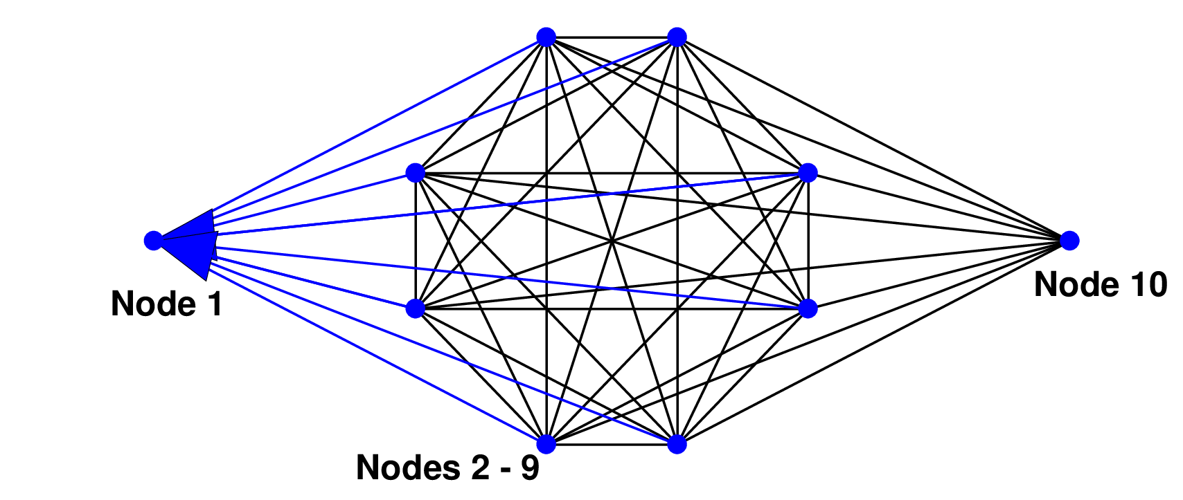
We demonstrate the differences between Protocols 2 and 2A through two examples. The first is related to the graph conditions in the two theorems. Consider networks with ten agents () with one mobile malicious agent (). It is easy to check that in this case, the conditions for Protocol 2 in Theorem IV.1 are satisfied only under the complete graph since the required number of neighbors for each agent is . On the other hand, the non-complete graph shown in Fig. 5 with ten nodes is -robust and thus satisfies the condition with for Protocol 2A in Theorem VI.1. In this graph, nodes 2–10 form a clique (i.e., a complete subgraph), but among them, only nodes 2–9 have directed edges (in blue) towards agent 1. Note that all agents have only eight (incoming) neighbors.

In the next example, we illustrate how Protocol 2A can achieve resilient consensus while Protocol 2 cannot because of the difference in their update rules. Here, we consider the graph shown in Fig 6 with six agents with one mobile malicious node (i.e., ). For our purpose, a simple graph is taken, which does not satisfy the theoretical conditions. The graph has two nodes having two neighbors and four nodes having four neighbors; among the latter four nodes, the malicious agent moves around periodically, following the M2 model. Note that the regular agents take only positive values while the malicious agent always takes , which results in the cured agent with take the same negative value.
At the initial step, one malicious agent and one cured agent are present indicated by red and green, respectively. In Fig 6, the left-most plot shows the status of the agents and their values chosen as at the start of round . Note the only agent not in consensus at this time is the agent on the far right of the graph taking the initial value ; this agent will be called agent 1 with value . After the initial round, as shown in Fig 6 on the right side, the malicious agent moves periodically among four agents in this network. Under Protocol 2, the updates will fail even at the initial round. With , agent 1 cannot update its value since it must have at least four values from its neighbors.
On the other hand, in Protocol 2A, each regular agent employs an update rule based on the conventional MSR algorithm. It hence always keeps and uses its own value in the updates. Thus, at round , agent 1 keeps its value unchanged as , removing the value received from the malicious agent. In fact, it remains unchanged in the following two rounds as , because it does not receive enough values because of the cured neighbors. At round , for the first time, agent 1’s value changes to by taking average of , , and . by taking average of and since the value is discarded by the protocol. Due to the periodic change in the values, we can show that agent 1 will update its value at rounds as for . while the values of other regular agents remain at 1. Clearly, it holds as , and thus resilient consensus will be achieved.
VI-C2 Network Conditions and Their Robustness
Next, we would like to relate the graph conditions obtained in Theorems III.1, IV.1, and V.1 with robust graphs. The following result provides the means to do so.
Proposition VI.1
For a given graph and a nonnegative integer , if the number of neighbors for each node satisfies , then this graph is -robust, where can be an arbitrary nonnegative integer.
Proof: At first, we take two disjoint subsets and of the node set with . There are two cases: (i) contains less than or equal to agents, and contains no fewer than agents. (ii) Both and contain less than agents. It is noted that one of these sets must contain less than or equal to agents. Then, we check every agent in . Since the number of its neighbors satisfies , we easily see that every agent inside must have at least neighbors from outside . Hence, the condition 1 or 2 in Definition II.1 must be satisfied. Since we do not need to check condition 3, the parameter can be chosen arbitrarily.
This result demonstrates that the graph conditions of Theorems III.1, IV.1, and V.1 can be stated in terms of robust graphs. We know that checking the robustness of large graphs is combinatorial and thus challenging. This proposition provides a simple analytic method to design networks with robustness properties.
Table II summarizes the properties of the five protocols under the four adversary models discussed in this paper including the conventional MSR algorithm under the static model. As shown in the table, for example, graphs satisfying the conditions for Protocol 1 in Theorem III.1 have the property of -robustness with any . Note however that this is only a necessary condition, and the converse does not hold in general. That is, in -robust graphs, each node does not necessarily satisfy . Further, from Table II, we can find that as the mobile adversarial model becomes more powerful, the required connectivity level also increases. This table also gives a comparison between the conventional MSR for static models and our proposed protocols for mobile models.
VII Numerical Example
In this section, we illustrate the performance of our proposed protocols and the conventional MSR algorithm under mobile adversary models through a numerical example using a wireless multi-agent network.
Our focus of the numerical experiments is to determine how well the protocols perform under practical settings when the assumptions introduced in the theoretical development may not hold. Specifically, we use randomly generated networks where the connectivity requirements are in general difficult to check due to the size of the network. Furthermore, we consider uncertain situations regarding the information of the adversarial agents in terms of their models and numbers. To this end, we use random graphs with 100 nodes and change the connectivity levels to examine the success rates for achieving resilient consensus through extensive simulations. We also check the cases where the parameter for the number of adversaries may be smaller than the actual number of such nodes; the latter number is denoted by in this section.

For the network topologies, we generated ten random geometric graphs with 100 nodes located in an area of meters meters randomly under the uniform distribution. Each agent has a communication range determined by the radius , within which it can communicate with all agents. An example is shown in Fig. 7 where the communication radius is chosen as . The regular agents and their edges are drawn in blue while the malicious agents are in red. Here, we placed 5 malicious agents, that is, .
In the box plot of Fig. 8, we display the distribution of the number of each agent’s neighbors for the topology in Fig. 7 versus the radius . For each , the green and blue curves indicate the maximum and the minimum numbers of neighbors, respectively, while the box represents the range containing the first to third quartiles and the line in the box shows the median. For large values of , a few red crosses are shown, indicating outliers.
In this experiment, we ran the algorithms under three settings to examine the success rates for resilient consensus. Throughout the simulations, the regular nodes’ initial values were randomly chosen under uniform distribution in the interval . On the other hand, the adversary nodes were given negative values so that their influence is easy to see. For the mobile adversaries, we used the random model, under which at each time step, the malicious agents randomly choose nodes to move from the entire network.

VII-A Consensus under Different Communication Radii
As we have observed in the theoretical results, the different models in the adversaries require different levels of connectivities in the network. In the first part of the simulations, we verify such properties of the algorithms by finding the smallest communication radius over which resilient consensus becomes possible. Such a communication radius will be referred to as the threshold radius.


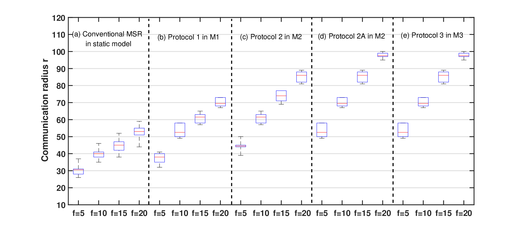
In the simulations, we examined the five cases as follows: (a) Conventional MSR protocol under the static model, (b) Protocol 1 under the M1 model, (c) Protocol 2 under the M2 model, (d) Protocol 2A under the M2 model, and (e) Protocol 3 under the M3 model. For each protocol, we checked four cases with the parameters , where the actual numbers of adversaries were taken as . The results are summarized in Fig. 9, where the threshold radii are shown for the five cases (a)–(e) from the left to right; the figure is given in the box plot style for the 10 network topologies generated as explained above.
We can observe two general trends in the results: First, for each protocol, as the number of adversaries increases, the threshold radius becomes larger. In the plots, the increase in the threshold size seems to be linear in for all five protocols. Second, the malicious nature in the models of the adversaries gradually becomes higher in the following order: the static model, M1, M2, and M3. Correspondingly, in the plots, we can confirm that from case (a) to case (d), the required levels of the threshold radii become larger.
It is interesting that when we compare the cases (c) for Protocol 2 and (e) for Protocol 2A, which are both for the same model M2, the thresholds are different. In fact, those for Protocol 2A are larger, being comparable to those for Protocol 3 under M3. This is because of the two cured rounds required in Protocol 2A since these rounds lead the network to be less connected. Recall that in Protocol 2A, the number of agents not sending their values can be up to , while in Protocol 2, it is up to . More specifically, in Protocol 2A, the regular agents and the cured agents with remove less neighbor information than the regular agents in Protocol 2. On the other hand, the cured agents in in Protocol 2A remove the same numbers of neighbors as those in Protocol 2.
We further note that the threshold results for cases (d) and (e) exactly coincide though the adversary models as well as the protocols are different. This is rather due to the special set up in the current simulations. In case (d) for Protocol 3, each regular agent always removes values from those received from neighbors. On the other hand, in case (e) under the model M3, cured agents do not send their values. Hence, since the malicious agents take negative values, the regular agents employing Protocol 2A or 3 under the corresponding model are always successful in ignoring the malicious agents’ values, resulting in the same behaviors and thus the same threshold values.
VII-B When the Number of Malicious Agents is Unknown
In the first part of the simulations, we have assumed that the number of the malicious agents in the network is known, that is, . In this second part, we check the performance of proposed algorithms when this does not hold, that is, the parameter used in the algorithm does not match the actual number of malicious agents. Here, we fixed the parameter in the protocols at and computed the success rates of resilient consensus by changing two parameters: the number of real malicious agents as and the communication radius as . In Fig. 10, the results are shown in the heat map format for the five cases (a)–(e) as in the previous part.
These plots reveal the sharp difference between the static and mobile malicious models. Fig. 10(a) shows the results of the conventional MSR algorithm under the static malicious model. We can see that the success rate is quite low with as the connectivity in the network is not enough. With , however, enough connectivity is introduced in the networks, and resilient consensus can be guaranteed in most topologies when .
Moreover, under the static malicious model, an interesting phenomenon occurs when more malicious agents exist in the network with . Observe that the success rate is high when . In this range, the communication radius is relatively small. Low connectivity in the network actually helps the regular agents since there are certain chances for each regular agent to receive fewer than malicious values. The conventional MSR is then able to achieve resilient consensus.
In contrast, under any of the mobile malicious models, this does not happen, and it is critical to take the parameter large enough that holds. In fact, in Figs. 10(b)–10(d), the success rates almost immediately go to 0 once . In the mobile models, the adversaries can switch among agents in the network, so once holds, there is a large chance that the regular agents receive more than malicious values at some time instants. After such moments, resilient consensus becomes impossible to reach. Thus, in mobile models, resilient consensus is very hard to guarantee when .
Furthermore, according to the malicious models, the sizes of the region indicating high success rates are different. As we have already seen in the previous part, the success rate becomes lower as the model becomes more adversarial from case (b) to case (e). It is interesting that under the model M2, for both Protocols 2 and 2A in Figs. 10(c) and Fig. 10(d), respectively, the success rates are affected by the size of even when the relation holds. This is because depending on the size of , the number of cured agents is determined. Hence, as increases, the overall system is under more uncertainties and its performance becomes worse. Note that even between these two protocols, the decrease in the success rates is different. Compared with the heat map for Protocol 2 in Fig. 10(c), the one for Protocol 2A in Fig. 10(d) indicates that the yellow region shrinks faster for larger . On the other hand, in the results for Protocols 1 and 3 in Figs. 10(b) and Fig. 10(e), respectively, the size of the parameter has much less impact on the chances of achieving resilient consensus. The reason is that in both protocols, the regular agents always ignore values at each update and this number stays the same regardless of the values received.
VII-C When the Mobile Malicious Model is Unknown
In the third part of the simulations, we introduce further uncertainties in the setting. In addition to using the actual number of malicious agents greater than the parameter used in the algorithms, we run the five protocols under different mobile models. As in the previous part, we fix the parameter as . Then, for two sets of network topologies, namely, with communication radius and , we performed simulations to calculate the success rates of resilient consensus by changing from 0 to 10. For each case, the maximum under which resilient consensus is reached in all 10 topologies was recorded. The results are displayed in Tables III (a) and III (b) for and , respectively.
In what follows, we discuss the case of with more connectivities among the agents for the four adversary models:
(i) In the static model, all five protocols can achieve resilient consensus under the 10 network topologies when the number of malicious agents in the network is less than the bound, i.e., . Protocol 3 is special in that it can tolerate up to malicious agents; this is because it ignores largest and smallest neighbor values.
(ii) For the mobile model M1, we can check that the conventional MSR fails to reach consensus as soon as one malicious agent is introduced (with ). In the meantime, the proposed protocols perform well for this mobile model when . Again, Protocol 3 can further tolerate up to malicious agents. Once the number exceeds the bound (or for Protocol 3), all protocols fail to reach resilient consensus for any of the topologies.
(iii) For the mobile M2, it is clear that the conventional MSR and Protocol 1 fail to reach consensus even with one malicious agent in the network while other protocols work well. Note that in this mobile model, Protocol 3 can tolerate only up to malicious agents. Recall that the models M2 and M3 share similar mobile behaviors, where the difference is that in M2, agents in the cured rounds are aware. However, Protocol 3 does not use this information and thus works the same as the case of M3. In both models, there may be malicious values in the system in each round. The success rates for all protocols go to zero when .
(iv) Finally, we checked the performance under M3. It is evident that except for Protocol 3, all protocols fail to reach consensus even with one malicious agent. As seen in Fig. 10(e), Protocol 3 is capable when sufficient connectivity is available, but cannot tolerate more malicious agents than the bound .
We now turn our attention to the case with the smaller communication radius. We have seen in Table III (a) that Protocol 3 can deal with all models when , but this capability is realized by requiring a high level of connectivities. It turns out that with , the network is not connected enough for Protocol 3, and it performs much worse than other protocols. In fact, as shown in Table III (b), Protocol 3 cannot reach consensus in any of the 10 topologies. The conventional MSR, Protocols 1 and 2 have similar performance as in the previous case with . Protocol 2A has some differences in M2 in that resilient consensus can be guaranteed in all 10 topologies when . Because of the mobile behavior in M2, the increase in can lead to the increase in cured agents at each round. Protocol 2A may have cured agents in one round. The cured agents do not send their values, which can reduce the connectivities.
We summarize the three simulation parts discussed in this section. The malicious agents become more adversarial according to the order in their models: The static, M1, M2, and M3. Protocols designed for more adversarial models are capable to deal with agents under less powerful models. For example, all mobile protocols can handle the static model, but the conventional MSR cannot reach consensus under any mobile models. We also confirmed through these simulations that protocols designed for more adversarial models require more connectivities to guarantee resilient consensus. These trade-offs are intuitive and can help the design of network structures for resilient consensus.
(a) With larger communication radius
Adversary model
Algorithm
Static
M1
M2
M3
Conventional MSR
Protocol 1
Protocol 2
Protocol 2A
Protocol 3
(b) With smaller communication radius
Adversary model
Algorithm
Static
M1
M2
M3
Conventional MSR
Protocol 1
Protocol 2
Protocol 2A
Protocol 3
VIII Conclusion
In this paper, we have considered the multi-agent consensus problem in the presence of mobile misbehaving agents and have developed resilient protocols to mitigate their influence on the regular agents. Specifically, under three classes of mobile malicious agents, four protocols have been proposed. For the protocols to achieve resilient consensus, we have characterized the conditions on the necessary graph structures through theoretical analyses under networks in both complete and non-complete graph forms. We have observed that these conditions reflect the different levels of adversarial capabilities that the three classes of mobile malicious agents possess. By means of numerical simulations, we have further studied the performance of the proposed resilient consensus protocols for random networks of 100 nodes where the theoretical conditions may not hold.
In future research, we will focus on formulating more detailed models for mobile adversary behaviors. We would also like to extend our approach to other multi-agent tasks where the adversary’s mobile capabilities may create complexity in the responses and actions of the regular agents for protecting the overall system. Furthermore, asynchronous update behaviors as well as time delays in communication should be taken into account.
References
- [1] M. H. Azadmanesh and R. M. Kieckhafer. Exploiting omissive faults in synchronous approximate agreement. IEEE Trans. Computers, 49(10), 1031–1042, 2000.
- [2] N. Banu, S. Souissi, T. Izumi, and K. Wada. An improved Byzantine agreement algorithm for synchronous systems with mobile faults. Int. J. Computer Applications, 43(21), 1–7, 2011.
- [3] F. Bonnet, X. Défago, T. D. Nguyen, and M. Potop-Butucaru. Tight bound on mobile Byzantine agreement. Theoretical Computer Science, 609, 361–373, 2016.
- [4] S. Bonomi, A. D. Pozzo, M. Potop-Butucaru, and S. Tixeuil. Approximate agreement under mobile Byzantine faults. Theoretical Computer Science, 758, 17–29, 2019.
- [5] Z. Bouzid, M. Potop-Butucaru, and S. Tixeuil. Optimal Byzantine-resilient convergence in uni-dimensional robot networks. Theoretical Computer Science, 411, 3154–3168, 2010.
- [6] S. Buhrman, J. A. Garay, and J. H. Hoepman. Optimal resiliency against mobile faults. In Proc. 25th Int. Symp. Fault-Tolerant Computing, 83–88, 1995.
- [7] F. Bullo. Lectures on Network Systems. Kindle Direct Publishing, 2019.
- [8] Y. Chen, S. Kar, and J. M. F. Moura. The Internet of Things: Secure distributed inference. IEEE Signal Processing Magazine, 35(5), 64–75, 2018.
- [9] S. M. Dibaji and H. Ishii. Consensus of second-order multi-agent systems in the presence of locally bounded faults. Systems & Control Letters, 79, 23–29, 2015.
- [10] S. M. Dibaji and H. Ishii. Resilient consensus of second-order agent networks: Asynchronous update rules with delays. Automatica, 81, 123–132, 2017.
- [11] S. M. Dibaji, H. Ishii, and R. Tempo. Resilient randomized quantized consensus. IEEE Trans. Automatic Control, 63(8), 2508–2522, 2018.
- [12] D. Dolev, N. A. Lynch, S. S. Pinter, W. E. Stark, and E. W. Weihl. Reaching approximate agreement in the presence of faults. J. ACM, 33(3), 499–516, 1986.
- [13] D. Fiore and G. Russo. Resilient consensus for multi-agent systems subject to differential privacy requirements. Automatica, 106, 18–26, 2019.
- [14] J. A. Garay. Reaching (and maintaining) agreement in the presence of mobile faults. In G. Tel and P. Vitányi (editors), Distributed Algorithms WDAG 1994. Lecture Notes in Computer Science, 857, Springer, 1994.
- [15] L. Guerrero-Bonilla, A. Prorok, and V. Kumar. Formations for resilient robot teams. IEEE Robotics and Automation Letters, 2(2), 841–848, 2017.
- [16] J. He, J. Chen, P. Cheng, and X. Cao. Secure time synchronization in wireless sensor networks: A maximum consensus-based approach. IEEE Trans. Parallel and Distributed Systems, 25(4), 1055–1065.
- [17] R. M. Kieckhafer and M. H. Azadmanesh. Reaching approximate agreement with mixed-mode faults. IEEE Trans. Parallel and Distributed Systems, 5(1), 53–63, 1994.
- [18] L. Lamport, R. Shostak, and M. Pease. The Byzantine generals problem. ACM Trans. Programming Languages and Systems, 4(3), 382–401, 1982.
- [19] H. J. LeBlanc, H. Zhang, X. Koutsoukos, and S. Sundaram. Resilient asymptotic consensus in robust networks. IEEE J. Selected Areas Comm., 31, 766–781, 2013.
- [20] C. Li, M. Hurfin, and Y. Wang. Reputation propagation and updating in mobile ad hoc networks with Byzantine failures. In Proc. IEEE Trustcom/BigDataSE/ISPA, 111–118, 2015.
- [21] N. A. Lynch Distributed Algorithms. Morgan Kaufmann, 1996.
- [22] M. Mesbahi and M. Egerstedt. Graph Theoretical Methods in Multiagent Networks. Princeton Univ. Press, 2010.
- [23] C. Nowzari, V. M. Preciado, and G. J. Pappas. Analysis and control of epidemics: A survey of spreading processes on complex networks. IEEE Control Systems Magazine, 36(1), 26–46, 2016.
- [24] R. Ostrovsky and M. Yung. How to withstand mobile virus attacks. In Proc. ACM Symp. Principles of Distributed Computing, 51–59, 1991.
- [25] H. Park and S. A. Hutchinson. Fault-tolerant rendezvous of multirobot systems. IEEE Trans. Robotics, 33(3), 565–582, 2017.
- [26] H. Sandberg, S. Amin, and K. H. Johansson (Guest editors). Special issue on cyberphysical security in networked control systems. IEEE Control Systems Magazine, 35(1), 2015.
- [27] T. Sasaki, Y. Yamauchi, S. Kijima, and M. Yamashita. Mobile Byzantine agreement on arbitrary network. In Proc. 17th Int. Conference on Principles of Distributed Systems, 236–250, 2013.
- [28] D. Sakavalas and L. Tseng. Delivery Delay and Mobile Faults. In Proc. IEEE 17th Int. Symp. on Network Computing and Applications (NCA), 1–8, 2018.
- [29] D. M. Senejohnny, S. Sundaram, C. De Persis, and P. Tesi. Resilience against misbehaving nodes in asynchronous networks. Automatica, 104, 26–33, 2019.
- [30] L. Tseng. An improved approximate consensus algorithm in the presence of mobile faults. In Proc. Int. Symp. Stabilization, Safety, and Security of Distributed Systems, 109–125, 2017.
- [31] J. Usevitch and D. Panagou. Resilient leader-follower consensus to arbitrary reference values in time-varying graphs, IEEE Trans. Automatic Control, 65(4), 1755–1762, 2020.
- [32] N. H. Vaidya, L. Tseng, and G. Liang. Iterative approximate Byzantine consensus in arbitrary directed graphs. In Proc. ACM Symp. Principles of Distributed Computing, 365–374, 2012.
- [33] Y. Wang and H. Ishii. Resilient consensus through event-based communication. IEEE Trans. Control of Network Systems, 7(1), 471–482, 2020.
- [34] Y. Wang and H. Ishii. An event-triggered approach to quantized resilient consensus. Int. J. of Robust and Nonlinear Control, to appear, 2020.
- [35] Y. Wang, H. Ishii, F. Bonnet, and X. Défago, Resilient consensus against mobile malicious agents. In Proc. IFAC World Congress, to appear, 2020.
- [36] L. Yuan and H. Ishii. Resilient consensus with distributed fault detection, In Proc. 8th IFAC Workshop on Distributed Estimation and Control in Networked Systems (NecSys’19), 285–290, 2019.
- [37] M. Yung. The “mobile adversary” paradigm in distributed computation and systems. In Proc. ACM Symp. Principles of Distributed Computing, 171–172, 2015.
- [38] H. Zhang, E. Fata, and S. Sundaram. A notion of robustness in complex networks. IEEE Trans. Control of Network Systems, 2(3), 310–320, 2015.
| Yuan Wang Yuan Wang received the M.Sc. degree in engineering from Huazhong University of Science and Technology, Wuhan, China in 2016, and the Ph.D. degree in Artificial Intelligence from Tokyo Institute of Technology, Yokohama, Japan in 2019. He is currently a researcher in the Department of Computer Science, Tokyo Institute of Technology, Yokohama, Japan. His main research interests are cyber-physical systems, event-based coordination, security in multi-agent systems, and model predictive control methods. |
| Hideaki Ishii (M’02-SM’12) received the M.Eng. degree in applied systems science from Kyoto University, Kyoto, Japan, in 1998, and the Ph.D. degree in electrical and computer engineering from the University of Toronto, Toronto, ON, Canada, in 2002. He was a Postdoctoral Research Associate with the Coordinated Science Laboratory at the University of Illinois at Urbana-Champaign, Urbana, IL, USA, from 2001 to 2004, and a Research Associate with the Department of Information Physics and Computing, The University of Tokyo, Tokyo, Japan, from 2004 to 2007. Currently, he is an Associate Professor in the Department of Computer Science, Tokyo Institute of Technology, Yokohama, Japan. His research interests are in networked control systems, multiagent systems, cyber security of power systems, and distributed and probabilistic algorithms. Dr. Ishii has served as an Associate Editor for the IEEE Control Systems Letters and the Mathematics of Control, Signals, and Systems and previously for Automatica, the IEEE Transactions on Automatic Control, and the IEEE Transactions on Control of Network Systems. He is the Chair of the IFAC Coordinating Committee on Systems and Signals since 2017. He received the IEEE Control Systems Magazine Outstanding Paper Award in 2015. |
| François Bonnet François Bonnet is a Specially Appointed Associated Professor at Tokyo Tech since 2018. He obtained his M.S. from the ENS Cachan at Rennes, France in 2006 and his Ph.D. from the University of Rennes 1 in 2010. He worked at JAIST as a JSPS postdoctoral fellow until 2012 and then as an Assistant Professor until 2017. Then he spent one year as a Specially Appointed Assistant Professor at Osaka University. His research interests include theoretical distributed computing, discrete algorithms, and (combinatorial) game theory. |
| Xavier Défago Xavier Défago is a full professor at Tokyo Institute of Technology since 2016. He obtained master (1995) and PhD (2000) in computer science from the Swiss Federal Institute of Technology in Lausanne (EPFL) in Switzerland. Before his current position at Tokyo Tech, he was a faculty member at the Japan Advanced Institute of Science and Technology (JAIST). Meanwhile, he has also been a PRESTO researcher for the Japan Science and Technology Agency (JST), and an invited researcher for CNRS (France) at Sorbonne University and at INRIA Sophia Antipolis. He is a member of the IFIP working group 10.4 on dependable computing and fault-tolerance. He served as program chair of IEEE SRDS in 2014 and IEEE ICDCS in 2012 and as general chair of SSS 2018. Xavier has been working on various aspects of dependable computing such as distributed agreement, state machine replication, failure detection, and fault-tolerant group communication in general. His interest include also robotics, embedded systems, and programming languages. |