An Empirical Process Approach to the Union Bound: Practical Algorithms for Combinatorial and Linear Bandits

The pure exploration stochastic multi-armed bandit (MAB) problem has received attention in recent years because it offers a useful framework for designing algorithms for sequential experiments. In this paper, we consider a very general formulation of the pure exploration MAB problem, namely, pure exploration (transductive) linear bandits [12] : given a set of measurement vectors $\mathcal{X}\subset\mathbb{R}^{d}$, a set of candidate items $\mathcal{Z}\subset\mathbb{R}^{d}$, and an unknown parameter vector $\theta\in\mathbb{R}^{d}$, an agent plays a sequential game where at each round she chooses a measurement vector $x\in\mathcal{X}$ and observes a stochastic random variable whose expected value is $\langle x,\theta\rangle$. The goal is to identify $z_{*}\in\argmax_{z\in\mathcal{Z}}\langle z,\theta\rangle$. This problem generalizes many well-studied problems in the literature including best arm identification [11, 21, 23, 25, 6], Top-K arm identification [22, 28, 9], the thresholding bandit problem [27], combinatorial bandits [10, 13, 8, 5, 20], and linear bandits where $\mathcal{X}=\mathcal{Z}$ [30, 33, 31].

The recent work of [12] proposed an algorithm that is within a $\log(|\mathcal{Z}|)$ multiplicative factor of previously known lower bounds [30] on the sample complexity. This term reflects a naive union bound over all informative directions $\{z_{*}-z:z\in\mathcal{Z}\setminus\{z_{*}\}\}$. Although one might be inclined to dismiss $\log(|\mathcal{Z}|)$ as a small factor, in many practical problems it can be extremely large. For example, in Top-K $\log(|\mathcal{Z}|)=\Theta(k\log(d))$ which would introduce an additional factor of $k$ that does not appear in the upper bounds of specialized algorithms for this class [22, 8, 25]. As another example, if $\mathcal{Z}$ consists of many vectors pointing in nearly the same direction, $\log(|\mathcal{Z}|)$ can be arbitrarily large, while we show that the true sample complexity does not depend on $\log(|\mathcal{Z}|)$. Finally, in many applications of linear bandits such as content recommendation $|\mathcal{Z}|$ can be enormous and thus the factor $\log(|\mathcal{Z}|)$ can have a dramatic effect on the sample complexity.

The high-level goal of this paper is to study how the geometry of the measurement vectors $\mathcal{X}$ and the candidate items $\mathcal{Z}$ influences the sample complexity of the pure exploration transductive linear bandit problem in the moderate confidence regime. We appeal to the fundamental TIS-inequality [19] which describes the deviation of the suprema of a Gaussian process from its expectation, leading us to propose an experimental design based on minimizing the expected suprema. We make the following contributions. First, we show a novel lower bound for the non-interactive oracle MLE algorithm, which devises a fixed sampling scheme using knowledge of $\theta$. While this non-interacting lower bound is not a lower bound for adaptive algorithms, it is suggestive of what union bounds are necessary and can be a multiplicative dimension factor larger than known adaptive lower bounds. Second, we develop a new algorithm for the fixed confidence setting (defined below) that nearly matches the performance of this oracle algorithm. Moreover, this algorithm recovers many of the state-of-the-art sample complexity results for combinatorial bandits as special cases. Third, applied specifically to the combinatorial bandit setting, we develop a practical and computationally efficient algorithm. We include experiments that show that our algorithm outperforms existing algorithms, often by an order of magnitude. Finally, we show that our techniques extend to the fixed budget setting where we provide the first fixed budget algorithm for transductive linear bandits. This algorithm matches the lower bound up to a factor that in most standard settings is bounded by $\log(d)$.

In the (transductive) linear bandit problem, the agent is given a set $\mathcal{X}\subset\mathbb{R}^{d}$ and a set of items $\mathcal{Z}\subset\mathbb{R}^{d}$. At each round $t$, an algorithm $\mathcal{A}$ selects a measurement $X_{t}\in\mathcal{X}$ which is measurable with respect to the history $\mathcal{F}_{t-1}=(X_{s},Y_{s})_{s<t}$ and observes a noisy observation $Y_{t}=X_{t}^{\top}\theta+\eta$ where $\theta\in\mathbb{R}^{d}$ is the unknown model parameter and $\eta$ is independent mean-0 Gaussian noise¹¹ 1 Our results still apply in the case where the noise is sub-Gaussian, but for simplicity here we assume that the noise is Gaussian (see the Supplementary Material).. We assume that $\text{argmax}_{z\in\mathcal{Z}}\langle z,\theta\rangle=\{z_{*}\}$, and the goal is to identify $z_{*}$. We consider two distinct settings.

Linear bandits is popular for applications such as content recommendation, digital advertisements, and A/B testing. For instance, in content recommendation $\mathcal{X}=\mathcal{Z}\subset\mathbb{R}^{d}$ may be sets of feature vectors describing songs (e.g., beats per minute, genre, etc.) and $\theta\in\mathbb{R}^{d}$ may represent an individual user’s preferences over the song library. An important sub-class of linear bandits is known as combinatorial bandits which is a focus of this work.

Combinatorial Bandits: In the combinatorial bandit setting, $\mathcal{X}=\{\mathbf{e}_{1},\ldots,\mathbf{e}_{d}\}$ (where $\mathbf{e}_{i}$ is the $i$-th canonical basis vector) and $\mathcal{Z}\subset\{0,1\}^{d}$. We will sometimes overload notation by treating $\mathcal{Z}$ as a collection of sets, e.g., for $z\in\mathcal{Z}$ writing $i\in z$ iff $\langle\mathbf{e}_{i},z\rangle=1$. We next give some examples of the combinatorial bandit setting.

In some of these settings, $|\mathcal{Z}|$ is exponential in the dimension $d$. For example, in the problem of finding a best matching in a bipartite graph, $|\mathcal{Z}|=(\sqrt{d})!$. In this setting a naive evaluation of $\text{argmax}_{z\in\mathcal{Z}}\langle z,\theta\rangle$ by enumerating $\mathcal{Z}$ becomes impossible even if $\theta$ were known. For such problems, we assume access to a linear maximization oracle

which is available in many cases, including matroids, matching, and identifying a shortest path in a directed acyclic graph (DAG). We will characterize the computational complexity of an algorithm in terms of the number of calls to the maximization oracle.

We now discuss how our work departs from previous approaches to the pure exploration linear bandit problem. Consider for a moment a fixed design where $n\geq d$ measurements $x_{1},\dots,x_{n}$ were decided before observing any data, and subsequently for each $1\leq i\leq n$ we observe $y_{i}=\langle x_{i},\theta\rangle+\eta_{i}$ with $\eta_{i}\sim\mathcal{N}(0,1)$. In this setting the maximum likelihood estimator (MLE) is given by ordinary least squares as $\widehat{\theta}=(\sum_{i=1}^{n}x_{i}x_{i}^{\top})^{-1}\sum_{i=1}^{n}y_{i}x_{i}$. Substituting the value of $y_{i}$ into this expression, we obtain $\widehat{\theta}=\theta+\left(\sum_{i=1}^{n}x_{i}x_{i}^{\top}\right)^{-1/2}\eta$ in distribution where $\eta\sim\mathcal{N}(0,I_{d})$. After collecting $\{(x_{i},y_{i})\}_{i=1}^{n}$ and computing $\widehat{\theta}$, the most reasonable estimate for $z_{\ast}=\arg\text{max}_{z\in\mathcal{Z}}\langle z,\theta\rangle$ is just $\widehat{z}=\arg\text{max}_{z\in\mathcal{Z}}\langle z,\widehat{\theta}\rangle$. The good event that $\widehat{z}=z_{\ast}$ occurs if and only if $\langle z_{\ast}-z,\widehat{\theta}\rangle>0$ for all $z\in\mathcal{Z}\setminus\{z_{\ast}\}$. Since $\widehat{\theta}$ is a Gaussian random vector, for each $z\in\mathcal{Z}$, $\langle z_{\ast}-z,\widehat{\theta}-\theta\rangle\sim\mathcal{N}(0,(z_{\ast}-z)^{\top}\left(\sum_{i=1}^{n}x_{i}x_{i}^{\top}\right)^{-1}(z_{\ast}-z))$. If we apply a standard sub-Gaussian tail-bound with a union bound over all $z\in\mathcal{Z}\setminus\{z_{*}\}$, then we have with probability greater than $1-\delta$ that

for all $z\in\mathcal{Z}\setminus\{z_{*}\}$ simultaneously, where we have taken $A=\sum_{i=1}^{n}x_{i}x_{i}^{\top}$ and used the notation $\|x\|_{W}^{2}=x^{\top}Wx$ for any square $W$. Thus, we conclude that if $n$ and $\{x_{1},\dots,x_{n}\}$ are chosen such that $\text{max}_{z\in\mathcal{Z}}\frac{\|z_{\ast}-z\|_{(\sum_{i=1}^{n}x_{i}x_{i}^{\top})^{-1}}^{2}}{\langle z_{\ast}-z,\theta^{*}\rangle^{2}}>2\log(|\mathcal{Z}|/\delta)$ then with probability at least $1-\delta$ we will have that $\langle z_{\ast}-z,\widehat{\theta}\rangle>0$ for all $z\in\mathcal{Z}$ and consequently, $\widehat{z}=z_{\ast}$. This simple argument is the core of all approaches to pure exploration linear bandits until this paper [30, 23, 33, 12]. However, applying a naive union bound over all $z\in\mathcal{Z}$ can be extremely weak and does not exploit the geometry of $\mathcal{Z}$ that induces many correlations among the random variables $\langle z_{\ast}-z,\widehat{\theta}\rangle$. At the heart of our approach is the following concentration inequality for the suprema of a Gaussian process (Theorem 5.8 in [2]).

Setting $\mathbb{S}=\mathcal{Z}$, we can apply this to the Gaussian process $V_{z}:=(z_{\ast}-z)^{\top}(\widehat{\theta}-\theta)=(z_{\ast}-z)^{\top}(\sum_{i=1}^{n}x_{i}x_{i}^{\top})^{-1/2}\eta$ where, again, $\eta\sim\mathcal{N}(0,I_{d})$. We then have with probability at least $1-\delta$

for all $z\in\mathcal{Z}\setminus\{z_{*}\}$ simultaneously. This bound naturally breaks into two components. The second-term is the high-probability term, and as the discussion above implies, naturally motivates the experimental design objective $\min_{x_{1},\cdots x_{n}}\text{max}_{z\in\mathcal{Z}\setminus\{z_{*}\}}\|z_{\ast}-z\|_{(\sum_{i=1}^{n}x_{i}x_{i}^{\top})^{-1}}^{2}$ from past works on linear-bandit pure exploration. The first term, $\mathbb{E}_{\eta\sim N(0,I_{d})}\left[\sup_{z\in\mathcal{Z}\setminus\{z_{*}\}}(z_{\ast}-z)^{\top}\left(\sum_{i=1}^{n}x_{i}x_{i}^{\top}\right)^{-1/2}\eta\right]$ is the Gaussian-width of the set $\{\left(\sum_{i=1}^{n}x_{i}x_{i}^{\top}\right)^{-1/2}(z_{\ast}-z)\}_{z\in\mathcal{Z}\setminus\{z_{*}\}}$ [32]. This term represents the penalty we pay for the union bound over the possible values of $\mathcal{Z}$ and reflects the underlying geometry of our arm set. For moderately sized values of $\delta\in(0,1)$ such as the science-stalwart $\delta=0.05$, the Gaussian width term can be substantially larger than the high probability term. Analogous to above, this motivates choosing $x_{1},\cdots,x_{n}$ to minimize the Gaussian width term.

Relaxation to Continuous Experimental Designs. In practice, optimizing over all finite sets of $\mathcal{X}$ of size $n$ to minimize an experimental design objective is NP-hard. Define $\simp:=\{\lambda\in\mathbb{R}^{|\mathcal{X}|}:\sum_{i}\lambda_{i}=1,\,\lambda_{i}\geq 0\}$ to be the simplex over elements $\mathcal{X}$ and define $A(\lambda)=\sum_{x\in\mathcal{X}}\lambda_{x}xx^{\top}$ where $\lambda\in\simp$ denotes a convex combination of the measurement vectors. Defining the design that minimizes the high probability term motivates the definition

On the other hand, minimizing the Gaussian width term motivates the definition

While the above suggests the importance of the quantities $\rho^{*}$ and $\gamma^{*}$, we will show later how they are intrinsic to the problem hardness. For now, we point out that these quantities are easily relatable.

Typically, $\inf_{z\neq z_{*}}\inf_{\lambda\in\simp}\tfrac{\left\lVert z_{*}-z\right\rVert^{2}_{A(\lambda)^{-1}}}{\langle\theta,z^{*}-z\rangle^{2}}\ll\rho^{*}$, in which case $\rho_{*}\lesssim\gamma_{*}$. While there are instances where $\gamma^{\ast}=\Theta(d\rho^{*})$, the upper bound is not necessarily tight.

This section formally justifies the quantities $\rho_{*}$ and $\gamma_{*}$ defined above. The following result holds for any $\mathcal{X}$ and $\mathcal{Z}$ and was first proven in this generality in [12], extending [30, 29, 8].

Mirroring the approaches developed in [24, 8, 14], it is possible to develop an algorithm that satisfies $\lim_{\delta\rightarrow 0}\frac{\mathbb{E}_{\theta}[\tau]}{\log(\frac{1}{\delta})}=\rho_{*}$, demonstrating the tightness of Theorem 2 in the regime of $\delta$ tending towards $0$. However, for fixed $\delta\in(0,1)$, algorithms for linear bandits to date have only been able to match this lower bound up to additive factors of $d\rho_{*}$ or $\log(|\mathcal{Z}|)\rho_{*}$ [24, 12] (note, this does not rule out optimality as $\delta\rightarrow 0$). In particular, the lower and the upper bounds of linear bandits do not reflect the underlying geometry of general sets $\mathcal{X}$ and $\mathcal{Z}$ in union bounds and are loose in general. For example, in the well-studied case of Top-K, these bounds do not capture some additive factors that are necessary and achievable in addition to $\rho_{*}$ alone [28, 9].

As a step towards characterizing the true sample complexity, we next demonstrate a lower bound that incorporates the geometry of $\mathcal{X}$ and $\mathcal{Z}$ for, presumably, the best possible non-interactive algorithm. Precisely, the procedure is given access to $\theta$, chooses an allocation $\{x_{I_{1}},x_{I_{2}},\dots\}\in\mathcal{X}$, then observes $\{y_{I_{1}},y_{I_{2}},\dots\}\in\mathbb{R}$ where $y_{I_{t}}\sim\mathcal{N}(\langle x_{I_{t}},\theta_{*}\rangle,1)$, and finally forms the MLE $\widehat{\theta}=\arg\min_{\theta}\sum_{t}(y_{I_{t}}-\langle x_{I_{t}},\theta\rangle)^{2}$ and outputs $\widehat{z}=\argmax_{z\in\mathcal{Z}}\langle z,\widehat{\theta}\rangle$. We emphasize that this procedure can pick any allocation it desires using full knowledge of $\theta$; in particular, it can use the allocation that achieves $\rho_{*}$.

By Proposition 2, $\gamma^{*}$ can be larger than $\rho^{*}$ by a multiplicative factor of the dimension $d$, demonstrating that the lower bound of Theorem 3 can be much larger than the lower bound of Theorem 2. While there exists problem instances in which the best known adaptive algorithm can achieve a sample complexity strictly smaller than the lower bound of Theorem 3 (e.g., best-arm identification), we are unaware of any settings in which the sample complexity of the best adaptive algorithm improves over Theorem 3 by more than a factor of $\log(d)$, which is typically considered insignificant.

In this section, we present Algorithm 1, Peace, that achieves the state-of-the-art sample complexity for (transductive) linear bandits in the fixed confidence setting. In each round $k$ we eliminate from the set of candidates $\mathcal{Z}$ all the elements that are roughly $2^{-k}$ suboptimal. In each round the query allocation is fixed according to the best non-adaptive strategy.

Our algorithm must round a design to an integral solution. It uses an efficient rounding procedure $\text{ROUND}(\lambda,N,\epsilon)$ that for $\lambda\in\simp$ and $N\geq q(\epsilon)$ returns $\kappa\in\mathbb{N}^{|\mathcal{X}|}$ such that $\sum_{x\in\mathcal{X}}\kappa_{x}=N$ and $\tau(\kappa;Z^{\prime})\leq(1+\epsilon)\tau(N\lambda;Z^{\prime})$ [1]. It suffices to take $q(\epsilon)=O(d/\epsilon^{2})$ (see the Supplementary Material). Define $S_{k}:=\{z\in\mathcal{Z}:\theta^{\top}(z^{*}-z)\leq B2^{-k}\}$, $\Delta_{z}:=\theta^{\top}(z_{*}-z)$, and $\Delta_{min}:=\min_{z\in\mathcal{Z}\setminus\{z_{*}\}}\Delta_{z}$.

We note that while our upper bound has an extra additive factor of $d$ compared to the lower bound of Theorem 3, this factor is necessary in many instances of interest (see the Supplementary Material). $\log(B)=O(\log(d))$ when $\mathcal{X}=\mathcal{Z}$ and in combinatorial bandits, and $B$ can be replaced by an upper bound on $\text{max}_{z\in\mathcal{Z}}\Delta_{z}$ when one is known. $\tau(\lambda;\mathcal{Z}_{k})$ can be optimized using stochastic mirror descent; we show that after a suitable transformation, it is convex in the combinatorial bandit setting. We conjecture that it is convex in the general case, as well.

Next, we turn to the fixed budget setting, where the goal is to minimize the probability of returning a suboptimal item $z\in\mathcal{Z}\setminus\{z_{*}\}$ given a budget of $T$ total measurements. Algorithm 3 is a generalization of the successive halving algorithm [23] and the first algorithm for fixed-budget linear bandits. It divides the budget into equally sized epochs and progressively shrinks the set of candidates $\mathcal{Z}_{k}$. In each epoch, it computes a design that minimizes $\gamma(\mathcal{Z}_{k})$ and samples according to a rounded solution. At the end of an epoch, it sorts the remaining items in $\mathcal{Z}_{k}$ by their estimated rewards and eliminates enough of the items with the smallest estimated rewards to ensure that $\gamma(\mathcal{Z}_{k+1})\leq\frac{\gamma(\mathcal{Z}_{k})}{2}$.

We note that the combinatorial bandit setting satisfies the assumption that $\gamma(\{z,z_{*}\})\geq 1$ for all $z\in\mathcal{Z}\setminus\{z_{*}\}$, but this lower bound is unessential and the algorithm can be modified to accommodate another lower bound. Theorem 6 implies that if $T\geq O(\log(1/\delta)[\rho^{*}+\gamma^{*}]\log(\gamma(\mathcal{Z}))\log(\log(\gamma(\mathcal{Z}))))$, then Algorithm 3 returns $z_{*}$ with probability at least $1-\delta$. Finally, $\log(\gamma(\mathcal{Z}))$ is $O(\log(d))$ in many cases, e.g., combinatorial bandits and in linear bandits when $\mathcal{X}=\mathcal{Z}$.

Transductive Linear Bandits: There is a long line of work in pure-exploration linear bandits [30, 33, 31] culminating in the formulation of the transductive linear bandit problem in [12] where the authors developed the first algorithm to provably achieve $\rho^{*}\log(|\mathcal{Z}|/\delta)$. The sample complexity of Theorem 4, $\gamma_{*}+\rho_{*}\log(1/\delta)$, is never worse than [12] since $\gamma_{*}\leq\rho_{*}\log(|\mathcal{Z}|)$ by Proposition 1. On the other hand, it is possible to come up with examples where $\gamma_{*}$ does not scale with $|\mathcal{Z}|$, but just $\rho_{*}$ (see experiments). While our algorithms work for arbitrary $\mathcal{X},\mathcal{Z}\subset\mathbb{R}^{d}$, problem instances of combinatorial bandits most clearly illustrate the advances of our new results over prior art.

Combinatorial Bandits: The pure exploration combinatorial bandit was introduced in [10], and followed by [13]. These papers are within a $\log(d)$ factor of the lower bound for the setting where $\mathcal{Z}$ is a matroid. If $\tilde{\Delta}_{i}=\theta^{\top}z_{*}-\text{max}_{z\in\mathcal{Z}:i\in z}\theta^{\top}z$ when $i\not\in z_{*}$ and $\theta^{\top}z_{*}-\text{max}_{z\in\mathcal{Z}:i\not\in z}\theta^{\top}z$ otherwise, then a lower bound is known to scale as $\sum_{i=1}^{d}\tilde{\Delta}_{i}^{-2}\log(1/\delta)$. The following result shows that $\gamma^{*}$ is within $\log(d)$ of the lower bound, implying that our sample complexity scales as $\sum_{i=1}^{d}\tilde{\Delta}_{i}^{-2}\log(d/\delta)$.

However, in the general setting where $\mathcal{Z}$ is not necessarily a matroid, [8] points out a class with $|\mathcal{Z}|=2$ where the sample complexity of [10, 13] is loose by a multiplicative factor of $d$. Chen et al. 2017a was the first to provide a lower bound equivalent to $\rho^{\ast}\log(1/\delta)$ for the general combinatorial bandit problem, as well as an upper bound of $\rho^{*}\log(|\mathcal{Z}|/\delta)$. However, as stressed in the current work, the $\log(|\mathcal{Z}|)$ term is not necessary in many scenarios; for example, in Top-K, $\rho^{*}\log(|\mathcal{Z}|)$ is larger than the best achievable sample complexity by a multiplicative factor of $k$ [9, 28]. This is not in contradiction with the lower bound provided in Theorem 1.9 of [8] which provides a specific worst-case class of instances where the $\log(|\mathcal{Z}|)$ is needed.

The next technological leap in combinatorial bandits is the algorithm of [5] (and the follow-up [20]). They provided an algorithm with a novel sample complexity that replaces $\log(|\mathcal{Z}|)$ with a more geometrically inspired term. Define the sphere $B(z,r)=\{z^{\prime}\in\mathcal{Z}:\left\lVert z-z^{\prime}\right\rVert_{2}=r\}$, and the complexity parameter $\varphi_{i}:=\text{max}_{z\in\mathcal{Z}\setminus\{z_{*}\}:i\in z^{*}\Delta z}\frac{\left\lVert z-z^{\prime}\right\rVert_{2}^{2}\log(d|B(z_{*},\left\lVert z-z^{\prime}\right\rVert_{2})|)}{\Delta_{z}^{2}}$. Then [5] provide a sample complexity scaling like $\varphi^{*}:=\sum_{i=1}^{n}\varphi_{i}$. The following shows that $\gamma^{\ast}$ is never more than $\log\log(d)$ larger than this complexity.

However, for even these sample complexity results that take the geometry into account, there exist clear examples of looseness that our approach avoids.

In summary, we have the first algorithm with a sample complexity that simultaneously is nearly optimal for matroids, essentially matches our novel lower bound $\gamma^{*}+\log(1/\delta)\rho^{*}\leq\log(|\mathcal{Z}|/\delta)\rho^{*}$, and is never worse than the sample complexity $\varphi^{*}$ from [5, 20].

Computational Results in Combinatorial Bandits: The algorithm CLUCB from [10] is computationally efficient and user-friendly. [5] and [8] provide computationally efficient algorithms, but these are impractical and we are unaware of any implementations of these algorithms.

Combinatorial Bandits: We compare Algorithm 2 against a uniform allocation strategy (UA) and CLUCB from [10]. We use $\delta=0.05$ on all the experiments and the empirical probability of failure never exceeded $\delta$ in all of our experiments. We consider two combinatorial structures.²² 2 We also outperform [5] on a bi-clique problem (see the Supplementary Material). (i) Matching: we use a balanced complete bipartite graph $G=(U\cup V,E)$ where $|U|=|V|=14$. Note that $|\mathcal{Z}|=14!\geq 8\cdot 10^{10}$. We took two disjoint matchings $M_{1}$ and $M_{2}$ and set $\theta_{e}=1$ if $e\in M_{1}$ and $\theta_{e}=1-h$ if $e\in M_{2}$ for $h\in\{.15,.1,.05,.025\}$. Otherwise, $\theta_{e}=0$. (ii) Shortest Path: we consider a DAG where a source leads into two disjoint feed-forward networks with 26 width-2 layers that then lead into a sink (see Figure 1 for an illustration). Note that $|\mathcal{Z}|\geq 10^{8}$. We consider two paths $P_{1}$ and $P_{2}$ such that they are in the disjoint feed-forward networks. We set $\theta_{e}=1$ if $e\in P_{1}$ and $\theta_{e}=1-h$ if $e\in P_{2}$ for $h\in\{.2,.15,.1,.05\}$. Otherwise, $\theta_{e}=-1$.

The first two panels of Figure 2 depict ratio of the average performance of the competing algorithms to the average performance of our algorithm. In the matching experiment, as the gap between the best matching $M_{1}$ and the second best matching $M_{2}$ get smaller, CLUCB pays a cost of roughly $|U|/h^{2}$ to distinguish $M_{1}$ from $M_{2}$ whereas our algorithm pays a cost of roughly $1/h^{2}$. A similar phenomenon occurs in the shortest path problem.

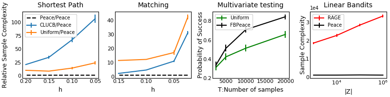
Multivariate Testing We consider multivariate testing [16, 15] in which there are $d$ options, each having $k$ possible levels. For example, consider determining the optimal content for a display-ad with slots such as headline, body, etc. and each slot has several variations. A layout is specified by a $d$-tuple $f=(f_{1},\cdots,f_{d})\in\{1,\cdots,k\}^{d}$ indicating the level chosen for each option. For each option $I$, $1\leq I\leq d$ and level $f$, $1\leq f\leq k$, there is a weight $W^{I}_{f}\in\mathbb{R}$, and for each pair of options $I,J$ and factors $f_{I},f_{J}$, there is a weight $W^{I,J}_{f_{I},f_{J}}\in\mathbb{R}$ capturing linear and quadratic interaction terms respectively. The total reward of a layout $f=(f_{1},\cdots,f_{d})$ is given by $W_{0}+\sum_{I=1}^{d}W^{I}_{f_{I}}+\sum_{I=1}^{d}\sum_{J=1}^{d}W^{I,J}_{f_{I},f_{J}}$. The fixed budget experiment in Figure 2 considers a scenario when $k=6$ and $d=3$ and compares Algorithm 3 (FBPeace) to uniform sampling. We set $W^{1,2}_{1,1}=.8$ and $W^{2,3}_{1,1}=.1$ and all other weights to zero, capturing a setting where the three options must be synchronized. At 10000 samples, FBPeace is 30% more likely to return the true optimal layout.

References

- Allen-Zhu et al. [2020] Zeyuan Allen-Zhu, Yuanzhi Li, Aarti Singh, and Yining Wang. Near-optimal discrete optimization for experimental design: A regret minimization approach. Mathematical Programming, pages 1–40, 2020.
- Boucheron et al. [2013] Stéphane Boucheron, Gábor Lugosi, and Pascal Massart. Concentration inequalities: A nonasymptotic theory of independence. Oxford university press, 2013.
- Brualdi [1969] Richard A Brualdi. Comments on bases in dependence structures. Bulletin of the Australian Mathematical Society, 1(2):161–167, 1969.
- Bubeck et al. [2015] Sébastien Bubeck et al. Convex optimization: Algorithms and complexity. Foundations and Trends® in Machine Learning, 8(3-4):231–357, 2015.
- Cao and Krishnamurthy [2019] Tongyi Cao and Akshay Krishnamurthy. Disagreement-based combinatorial pure exploration: Sample complexity bounds and an efficient algorithm. In Conference on Learning Theory, pages 558–588, 2019.
- Chen and Li [2015] Lijie Chen and Jian Li. On the optimal sample complexity for best arm identification. arXiv preprint arXiv:1511.03774, 2015.
- Chen et al. [2016] Lijie Chen, Anupam Gupta, and Jian Li. Pure exploration of multi-armed bandit under matroid constraints. In Conference on Learning Theory, pages 647–669, 2016.
- Chen et al. [2017a] Lijie Chen, Anupam Gupta, Jian Li, Mingda Qiao, and Ruosong Wang. Nearly optimal sampling algorithms for combinatorial pure exploration. In Conference on Learning Theory, pages 482–534, 2017a.
- Chen et al. [2017b] Lijie Chen, Jian Li, and Mingda Qiao. Nearly instance optimal sample complexity bounds for top-k arm selection. In Artificial Intelligence and Statistics, pages 101–110, 2017b.
- Chen et al. [2014] Shouyuan Chen, Tian Lin, Irwin King, Michael R Lyu, and Wei Chen. Combinatorial pure exploration of multi-armed bandits. In Advances in Neural Information Processing Systems, pages 379–387, 2014.
- Even-Dar et al. [2006] Eyal Even-Dar, Shie Mannor, and Yishay Mansour. Action elimination and stopping conditions for the multi-armed bandit and reinforcement learning problems. Journal of machine learning research, 7(Jun):1079–1105, 2006.
- Fiez et al. [2019] Tanner Fiez, Lalit Jain, Kevin G Jamieson, and Lillian Ratliff. Sequential experimental design for transductive linear bandits. In Advances in Neural Information Processing Systems, pages 10666–10676, 2019.
- Gabillon et al. [2016] Victor Gabillon, Alessandro Lazaric, Mohammad Ghavamzadeh, Ronald Ortner, and Peter Bartlett. Improved learning complexity in combinatorial pure exploration bandits. In Artificial Intelligence and Statistics, pages 1004–1012, 2016.
- Garivier and Kaufmann [2016] Aurélien Garivier and Emilie Kaufmann. Optimal best arm identification with fixed confidence. In Conference on Learning Theory, pages 998–1027, 2016.
- Heller [1986] Barbara Heller. Statistics for experimenters, an introduction to design, data analysis, and model building: GEP Box, WG Hunter and JS Hunter, John Wiley and Sons, New York, NY. 1978. Pergamon, 1986.
- Hill et al. [2017] Daniel N Hill, Houssam Nassif, Yi Liu, Anand Iyer, and SVN Vishwanathan. An efficient bandit algorithm for realtime multivariate optimization. In Proceedings of the 23rd ACM SIGKDD International Conference on Knowledge Discovery and Data Mining, pages 1813–1821, 2017.
- Howard et al. [2018] Steven R Howard, Aaditya Ramdas, Jon McAuliffe, and Jasjeet Sekhon. Uniform, nonparametric, non-asymptotic confidence sequences. arXiv preprint arXiv:1810.08240, 2018.
- Hsu and Sabato [2014] Daniel Hsu and Sivan Sabato. Heavy-tailed regression with a generalized median-of-means. In International Conference on Machine Learning, pages 37–45, 2014.
- Ibragimov et al. [1976] IA Ibragimov, VN Sudakov, and BS Tsirelson. Norms of gaussian sample functions. In Proceedings of the third Japan USSR symposium on probability theory, lecture notes in math, volume 550, pages 20–41, 1976.
- Jain and Jamieson [2019] Lalit Jain and Kevin G Jamieson. A new perspective on pool-based active classification and false-discovery control. In Advances in Neural Information Processing Systems, pages 13992–14003, 2019.
- Jamieson et al. [2014] Kevin Jamieson, Matthew Malloy, Robert Nowak, and Sébastien Bubeck. lil’ucb: An optimal exploration algorithm for multi-armed bandits. In Conference on Learning Theory, pages 423–439, 2014.
- Kalyanakrishnan et al. [2012] Shivaram Kalyanakrishnan, Ambuj Tewari, Peter Auer, and Peter Stone. PAC subset selection in stochastic multi-armed bandits. In Proceedings of the 29th International Conference on Machine Learning, ICML 2012, Edinburgh, Scotland, UK, June 26 - July 1, 2012, 2012.
- Karnin et al. [2013] Zohar Karnin, Tomer Koren, and Oren Somekh. Almost optimal exploration in multi-armed bandits. In Sanjoy Dasgupta and David Mcallester, editors, Proceedings of the 30th International Conference on Machine Learning (ICML-13), volume 28, pages 1238–1246. JMLR Workshop and Conference Proceedings, May 2013.
- Karnin [2016] Zohar S Karnin. Verification based solution for structured mab problems. In Advances in Neural Information Processing Systems, pages 145–153, 2016.
- Kaufmann et al. [2016] Emilie Kaufmann, Olivier Cappé, and Aurélien Garivier. On the complexity of best-arm identification in multi-armed bandit models. The Journal of Machine Learning Research, 17(1):1–42, 2016.
- Lattimore and Szepesvári [2020] Tor Lattimore and Csaba Szepesvári. Bandit Algorithms. Cambridge University Press, 2020.
- Locatelli et al. [2016] Andrea Locatelli, Maurilio Gutzeit, and Alexandra Carpentier. An optimal algorithm for the thresholding bandit problem. In International Conference on Machine Learning, pages 1690–1698, 2016.
- Simchowitz et al. [2017] Max Simchowitz, Kevin Jamieson, and Benjamin Recht. The simulator: Understanding adaptive sampling in the moderate-confidence regime. In Conference on Learning Theory, pages 1794–1834, 2017.
- Soare [2015] Marta Soare. Sequential resource allocation in linear stochastic bandits. PhD thesis, 2015.
- Soare et al. [2014] Marta Soare, Alessandro Lazaric, and Rémi Munos. Best-arm identification in linear bandits. In Advances in Neural Information Processing Systems, pages 828–836, 2014.
- Tao et al. [2018] Chao Tao, Saúl Blanco, and Yuan Zhou. Best arm identification in linear bandits with linear dimension dependency. In International Conference on Machine Learning, pages 4877–4886, 2018.
- Vershynin [2019] Roman Vershynin. High-Dimensional Probability. 2019.
- Xu et al. [2018] Liyuan Xu, Junya Honda, and Masashi Sugiyama. A fully adaptive algorithm for pure exploration in linear bandits. In International Conference on Artificial Intelligence and Statistics, pages 843–851, 2018.
Appendix A Outline and Notation
Section B gives the proof of Theorem 3. Section C presents proofs of the two results for the fixed confidence setting. Section D proves provides the main results on the computational efficiency of Algorithm 2. Section E provides the proof of our upper bound for the fixed budget setting. Section F proves various results related to . Section G gives additional lower bounds for the transductive linear bandit problem. Section H provides a discussion of rounding. Section I presents technical lemmas. Section J discusses the convexity of . Section K discusses the sample complexity results of other papers. Section M gives further details on the other experiments.
For the combinatorial bandit setting, we assume wlog that for all there exist such that and . We will sometimes write to denote . In a similar way, we will use to denote the symmetric difference of and , viewed as sets. We use to denote positive universal constants whose values may change from line to line.
Appendix B Proof of Theorem 3
Proof of Theorem 3.
Define . Let . Fix to be the measurement vectors pulled by the algorithm. Define the matrix
Define .
Let be the associated allocation: . Note that
and
Since are fixed, the same argument from the proof of Theorem 1 in [12] implies that since is -PAC,