Statistical Frameworks for Oncology Dose-Finding Designs with Late-Onset Toxicities: A ReviewThanks: 
Submitted to Statistical Science in December 2019

Phase I dose-finding studies are usually first-in-human trials for a new drug to go through before it can be approved for general use in the public. Oncology dose-finding trials aim to identify an efficacious dose with a tolerable level of toxicity, known as the maximum tolerated dose (MTD), which may be selected as the chosen dose for treating thousands of patients in subsequent clinical trials of later phases. The failure of determining an appropriate dose could lead to failure of later-phase trials and the final drug approval. Therefore, to increase the chance of identifying a safe and efficacious dose, dose-finding trials rely on efficient statistical designs and motivate several interesting statistical problems and challenges. First, oncology dose-finding trials are usually conducted with relatively small sample sizes (10 to 50 patients), which may not support statistical models of great complexity. Therefore, mainstream dose-finding designs are typically built upon relatively simple statistical models. Second, in dose-finding trials, safety concerns and ethical constraints often outplay statistical optimality in decision-making. Third, to reduce the enormous cost of new drug development, there has always been a need to shorten trial duration with advanced statistical tools. Dose-finding is a broad topic, and in this paper, we focus on the third problem of shortening trial duration by utilizing time-to-event information. It is estimated that a phase I clinical trial typically costs several thousand dollars a day to maintain its regular operation (see, e.g., Sertkaya et al., 2016). Therefore, financial savings on trial duration is very desirable. In addition, due to the competition in drug development, the race to being the first-in-class drug is also important, and shorter trials give a higher chance of being the first to go to market. For all these reasons and others that will be more clear next, novel statistical designs have been developed to speed up dose-finding trials.

Formally, the MTD is defined as the highest dose with toxicity probability close to or lower than a pre-specified target rate $p^{*}$. The type of toxicity is usually severe, like organ failure, and is called dose-limiting toxicity (DLT). The premise behind dose-finding trials is that both the toxicity and efficacy of a treatment monotonically increase with the dose level. A dose level that is too low can not provide needed efficacy, e.g. anti-tumor activity, while a dose level that is too high might induce severe toxicity. Therefore, it is crucial to find an appropriate dose that has the highest possible efficacy while maintains tolerable toxicity. Usually, a grid of discrete dose levels are investigated, and cohorts of patients are sequentially enrolled and adaptively treated at the ascending dose levels based on the previously observed data. The trial objectives include the identification of the MTD and the estimation of the dose-toxicity relationship, as well as maximizing the chance of treating patients at safe and efficacious doses.

The evaluation of DLT is conducted by following patients post-treatment within a time window, during which DLT outcomes and times to DLTs are recorded. If a patient does not experience any DLT during the follow-up window, the patient is declared having no DLT. Most existing designs require the DLT evaluation of all the previously enrolled patients to be completed before they can make a treatment assignment for the next cohort of patients. Consequently, we refer to this type of designs as complete-data designs. Examples of complete-data designs include the 3+3 design (Storer, 1989), continual reassessment method (CRM, O’Quigley et al., 1990; Goodman et al., 1995; Shen and O’Quigley, 1996; O’Quigley and Shen, 1996), escalation with overdose control (EWOC, Babb et al., 1998), product-of-beta prior method (PBP, Gasparini and Eisele, 2000), cumulative cohort design (CCD, Ivanova et al., 2007), Bayesian logistic regression model (BLRM, Neuenschwander et al., 2008), modified toxicity probability interval design (mTPI, Ji et al., 2010; Ji and Wang, 2013), product of independent beta probabilities escalation design (PIPE, Mander and Sweeting, 2015), Bayesian optimal interval design (BOIN, Liu and Yuan, 2015; Yuan et al., 2016), mTPI-2 design (Guo et al., 2017), keyboard design (Yan et al., 2017), semiparametric dose finding method (SPM, Clertant and O’Quigley, 2017; Clertant and O’Quigley, 2019), Bayesian uncertainty-directed design (BUD, Domenicano et al., 2019), surface-free design (SFD, Mozgunov et al., 2020), and i3+3 design (Liu et al., 2020), among many others. The majority of these designs are for single-agent dose-finding trials (i.e., a single investigational drug is studied), which are the focus of this article. For therapies of which the toxicity is acute and can be ascertained relatively quickly, such as cytotoxic chemotherapies, waiting for the DLT evaluation of previous patients may not be a concern, as the DLT assessment window can be short. However, for therapies that usually have late-onset toxicity, such as immunotherapies (Weber et al., 2015; Kanjanapan et al., 2019), it is more sensible to use a relatively long assessment window. This may cause difficulty for complete-data designs to operate, since patient enrollment needs to be frequently suspended until the previous patients have finished their assessment. The same difficulty arises when patient accrual is relatively fast compared to the length of the assessment window. For example, in Figure 1.1(a), while waiting for the DLT outcomes of the first 3 patients, new patient enrollment needs to be suspended, and 3 eligible patients have to be turned away. Trial suspension is undesirable in practice for two reasons. First, trial duration is prolonged, which delays scientific research and drug development. Second, subsequent patients that are available for enrollment need to be turned away, which results in a delay in their cancer care. Many patients participating in the trial do not have alternative choices for treatment, and the trial may be their last treatment option. Their diseases may also be in rapid deterioration, thus they are in need of immediate treatment.

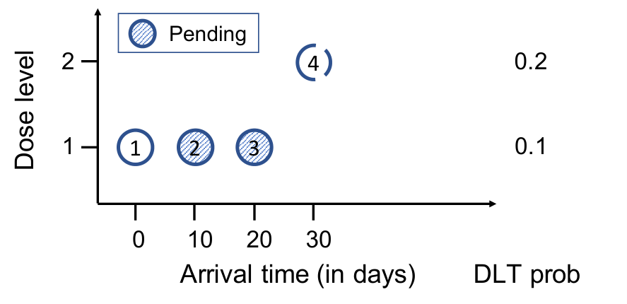
To address these practical concerns, several designs have been proposed to allow consecutive patient accrual even if some enrolled patients are still pending for DLT assessment. These include the time-to-event CRM (TITE-CRM, Cheung and Chappell, 2000; Normolle and Lawrence, 2006), rolling six design (R6, Skolnik et al., 2008), expectation-maximization CRM (EM-CRM, Yuan and Yin, 2011), data augmentation CRM (DA-CRM, Liu et al., 2013), time-to-event BOIN design (TITE-BOIN, Yuan et al., 2018), time-to-event PIPE design (TITE-PIPE, Wheeler et al., 2019), rolling TPI design (R-TPI, Guo et al., 2019), time-to-event keyboard design (TITE-keyboard, Lin and Yuan, 2020), and probability-of-decision TPI design (POD-TPI, Zhou et al., 2020). Except for R6 and R-TPI, these designs utilize time-to-event information to make treatment assignments thus are referred to as time-to-event designs. As an example, in Figure 1.1(b), when the 4th patient is available for enrollment, patients 2 and 3 are still being followed without definitive outcomes. Based on the DLT outcome of patient 1, time-to-DLT information of patient 1 and follow-up time information of patients 2 and 3, a time-to-event design may enroll the patient and de-escalate the dose level, which avoids the trial suspension.

In this article, we summarize the vast literature of time-to-event dose-finding designs into two general classes. See Figure 1.2. The key component is the construction of the likelihood function with time-to-event data, and the primary interest is inference on toxicity probabilities. Specifically, two equivalent modeling approaches can be taken for the likelihood construction. The statistical frameworks give rise to two classes of time-to-event designs, which contain the existing designs as special cases and also lead to new designs. The first class of time-to-event designs, called TITE designs, make dose-finding decisions based on inference on toxicity probabilities. The second class of time-to-event designs, called POD (probability of decision) designs, is a new type of designs that directly make inference on dose-finding decisions when DLT outcomes may be pending. The POD designs directly reflect the confidence of possible decisions and offer the investigators and regulators a way to properly assess and control the chance of making incompatible decisions when not all patients have been completely followed.

Along with the statistical frameworks, we introduce several computational algorithms to facilitate the use of time-to-event designs in practice. We discuss and study theoretical properties of time-to-event designs, such as large-sample convergence properties, coherence principles and the underlying decision rules, with a focus on interval-based and curve-free designs. We also review practical considerations of time-to-event designs, which are important in the execution of clinical trials. Usually, ad-hoc rules need to be imposed to ensure that the designs satisfy safety concerns and ethical constraints. Lastly, we examine finite-sample operating characteristics of some designs through computer simulations.

The remainder of the paper is structured as follows. In Section 2, we give a brief review of complete-data designs. In Section 3, we review statistical frameworks for time-to-event modeling in dose-finding trials. In Section 4, we introduce the two summarized classes of time-to-event designs: TITE and POD designs. In Section 5, we study theoretical properties of time-to-event designs. In Section 6, we discuss practical considerations. We assess the operating characteristics of several existing and newly proposed dose-finding designs under the TITE and POD frameworks via simulation studies in Section 7. Finally, we conclude with a discussion in Section 8. Technical details, including the computational algorithms and proof of the theoretical results, are provided in the appendix. The R source code for implementing several time-to-event designs and replicating the simulation studies is also provided as a supplementary file.

We start with a brief review of complete-data designs. At a given moment in a dose-finding trial, suppose $N$ patients have been treated, and the $(N+1)$th patient is eligible for enrollment. Let $Z_{i}\in\{1,\ldots,J\}$ denote the dose assigned to patient $i$, where $J$ is the number of available doses in the trial. Each patient is supposed to be followed for a fixed period of time $W$, and we use $Y_{i}=1$ or $0$ to represent the binary outcome of whether or not patient $i$ experiences DLT within the time window, respectively. For example, in many oncology trials, $W=28$ days. Let $p_{z}$ denote the probability of DLT at dose $z\in\{1,\ldots,J\}$ within the assessment window. The conditional distribution of $Y_{i}$ given $Z_{i}$ and $p_{z}$ is commonly modeled with a Bernoulli distribution,

A widely recognized assumption is that the DLT probability is monotone with the dose level, i.e. $p_{1}\leq p_{2}\leq\cdots\leq p_{J}$.

Suppose $Y_{i}$’s are fully observed for the first $N$ patients, and denote by $\mathcal{H}_{N}^{*}=\{(Y_{i},Z_{i}):i\leq N\}$ the previous history of observations. A complete-data design $\mathcal{A}^{*}$ can be viewed as a function of $\mathcal{H}_{N}^{*}$, which prescribes a dose $\mathcal{A}^{*}(\mathcal{H}_{N}^{*})$ for the new patient through two steps: (1) making inference about $p_{z}$’s, and (2) translating such inference to a dose-finding decision. As we shall see later, the monotonicity assumption of the DLT probabilities can play a role in both of these two steps. Inference on $p_{z}$’s can be based on the likelihood,

where $\bm{y}=(y_{1},\ldots,y_{N})$ and $\bm{z}=(z_{1},\ldots,z_{N})$ are the observed outcomes and dose assignments for the $N$ patients, respectively, and $\bm{p}=(p_{1},\ldots,p_{J})$ is the vector of toxicity probabilities. As mentioned in Section 1, there is a rich literature on complete-data dose-finding designs. The existing literature can be roughly divided into model-based and rule-based (i.e., model-free) designs (Zhou and Ji, 2020). Two classes of model-based designs, one using parametric dose-toxicity response curves and the other curve-free, accommodate the monotone dose-toxicity relationship with different approaches. The curve-based designs directly build the monotonicity assumption into the proposed curves, e.g., using a positive coefficient, while curve-free designs implicitly accommodate the assumption by an up-and-down decision framework. For example, when the observed toxicity data suggest that a dose is below or above the MTD target, the decision is to escalate (go up) or de-escalate (go down) the dose level, respectively. Below, we provide a brief review of six main-stream complete-data dose-finding designs: CRM, BOIN, mTPI-2, keyboard, SPM and i3+3. The 3+3 design is excluded from the discussion, as it does not allow the specification of a particular DLT target $p^{*}$ and a maximum sample size. It is widely recognized that 3+3 has worse performance than, e.g., mTPI (Ji and Wang, 2013). We denote by $N_{z}=\sum_{i=1}^{N}\mathbbm{1}(Z_{i}=z)$, $n_{z}=\sum_{i=1}^{N}\mathbbm{1}(Z_{i}=z,Y_{i}=1)$, and $m_{z}=\sum_{i=1}^{N}\mathbbm{1}(Z_{i}=z,Y_{i}=0)$ the total numbers of patients, DLTs, and non-DLTs at dose $z$, respectively.

Continual Reassessment Method (CRM):

The CRM design assumes a dose-toxicity response curve $p_{z}=\phi(z,\alpha)$, where $\alpha$ is an unknown parameter. Based on the monotonicity assumption of the DLT probabilities, $\phi$ should monotonically increase with $z$. For example, a commonly used dose-toxicity curve is $\phi(z,\alpha)=p_{0z}^{\exp(\alpha)}$, where $p_{0z}$’s are pre-specified constants satisfying $p_{01}<\cdots<p_{0D}$. The likelihood becomes

$\displaystyle L(\alpha\mid\mathcal{H}_{N}^{*})=\prod_{i=1}^{N}\phi(z_{i},\alpha)^{y_{i}}[1-\phi(z_{i},\alpha)]^{1-y_{i}}.$

Inference on $\alpha$ can be Bayesian (O’Quigley et al., 1990) or based on maximum likelihood (O’Quigley and Shen, 1996). From a Bayesian perspective, a prior distribution $\pi_{0}(\alpha)$ is specified for $\alpha$ (for example, $\alpha\sim\text{N}(0,1.34^{2})$), leading to the posterior $\pi(\alpha\mid\bm{y},\bm{z})\propto\pi_{0}(\alpha)L(\alpha\mid\bm{y},\bm{z})$. The DLT probabilities can thus be estimated by $\hat{p}_{z}=\int\phi(z,\alpha)\pi(\alpha\mid\bm{y},\bm{z})d\alpha$. On the other hand, the maximum likelihood estimate (MLE) for $\alpha$ is $\hat{\alpha}=\argmax_{\alpha}L(\alpha\mid\bm{y},\bm{z})$, and $p_{z}$ can be estimated by $\hat{p}_{z}=\phi(z,\hat{\alpha})$. In both cases, the dose $d^{*}=\argmin_{z}|\hat{p}_{z}-p^{*}|$ is recommended for the next patient, subject to some practical safety restrictions (Goodman et al., 1995; Cheung, 2005).

Bayesian Optimal Interval (BOIN) Design:

We refer to the local BOIN design (Liu and Yuan, 2015), which considers a statistical test of three hypotheses:

(2.3)

$\displaystyle H_{0}:p_{d}=p^{*},\quad H_{1}:p_{d}=p^{\text{L}},\quad H_{2}:p_{d}=p^{\text{R}}.$

Here $d$ is the current dose level, $p^{\text{L}}$ denotes the highest toxicity probability that is deemed subtherapeutic such that dose escalation should be made, and $p^{\text{R}}$ denotes the lowest toxicity probability that is deemed overly toxic such that dose de-escalation is required. The quantities $p^{\text{L}}$ and $p^{\text{R}}$ need to be pre-specified by physicians. Assuming equal prior weights on the three hypotheses, the optimal decision boundaries $\lambda^{\text{L}}(p^{*},p^{\text{L}})$ and $\lambda^{\text{R}}(p^{*},p^{\text{R}})$ minimizing the decision error rate are,

$\displaystyle\begin{split}\lambda^{\text{L}}&=\left.\log\left(\frac{1-p^{\text{L}}}{1-p^{*}}\right)\middle/\log\left[\frac{p^{*}(1-p^{\text{L}})}{p^{\text{L}}(1-p^{*})}\right]\right.,\\ \lambda^{\text{R}}&=\left.\log\left(\frac{1-p^{*}}{1-p^{\text{R}}}\right)\middle/\log\left[\frac{p^{\text{R}}(1-p^{*})}{p^{*}(1-p^{\text{R}})}\right]\right..\end{split}$

Let $\hat{p}_{d}=n_{d}/N_{d}$ denote the MLE for $p_{d}$. If $\hat{p}_{d}\leq\lambda^{\text{L}}$, the dose is escalated for the next patient; if $\hat{p}_{d}\geq\lambda^{\text{R}}$, the dose is de-escalated; otherwise, the same dose level is retained. Note that $\lambda^{\text{L}}$ and $\lambda^{\text{R}}$ can be pre-specified without the optimization procedure in Liu and Yuan, 2015. When they are pre-specified, BOIN uses essentially the same up-and-down rules as the cumulative cohort design (Ivanova et al., 2007). Although the monotonicity assumption of the DLT probabilities is not imposed on the inference of $p_{d}$, it plays a role in the dose-finding decision. For example, if $p_{d}$ is deemed lower than $p^{*}$, then a dose-escalation decision is made, because we believe the next higher dose level will have higher DLT and efficacy probabilities and may be closer to the MTD.

mTPI-2 Design:

The mTPI-2 design considers a partition of the $[0,1]$ interval into an equivalence interval $I_{\text{S}}=[p^{*}-\epsilon_{1},p^{*}+\epsilon_{2}]$, an underdosing interval $I_{\text{E}}=[0,p^{*}-\epsilon_{1})$, and an overdosing interval $I_{\text{D}}=(p^{*}+\epsilon_{2},1]$. Here, the subscripts “S”, “E”, and “D” stand for the corresponding dose-finding decisions: Stay, Escalation, and De-escalation. Any dose with toxicity probability inside $I_{\text{S}}$ is considered a true MTD and corresponds to a decision of “S”. The doses in $I_{\text{E}}$ (or $I_{\text{D}})$ are considered subtherapeutic (or overly toxic) and lower (or higher) than the MTD thus correspond to a decision of “E” (or “D”). The values $\epsilon_{1}$ and $\epsilon_{2}$ need to be specified by physicians. The intervals $I_{\text{E}}$ and $I_{\text{D}}$ are further divided into several sub-intervals, $I_{\text{E}_{0}},\ldots,I_{\text{E}_{K_{1}}}$ and $I_{\text{D}_{0}},\ldots,I_{\text{D}_{K_{2}}}$, such that all the sub-intervals have the same length $(\epsilon_{1}+\epsilon_{2})$ except for the two intervals ($I_{\text{E}_{0}}$ and $I_{\text{D}_{0}}$) reaching the boundary of $[0,1]$. Let $d$ denote the current dose level, and let model $\{\mathcal{M}_{d}=k\}$ represent $\{p_{d}\in I_{k}\}$, $k=\text{E}_{0},\ldots,\text{E}_{K_{1}},\text{S},\text{D}_{0},\ldots,\text{D}_{K_{2}}$. The mTPI-2 design is based on the following hierarchical prior model for $\mathcal{M}_{d}$ and $p_{d}$,

(2.4)

$\displaystyle\begin{split}&\Pr(\mathcal{M}_{d}=k)=1/(K_{1}+K_{2}+3),\;\text{for $k=\text{E}_{0},\ldots,\text{E}_{K_{1}},\text{S},\text{D}_{0},\ldots,\text{D}_{K_{2}}$};\\ &p_{d}\mid\mathcal{M}_{d}\sim\text{TBeta}(1,1;I_{\mathcal{M}_{d}}),\end{split}$

where $\text{TBeta}(\cdot,\cdot;I)$ represents a truncated beta distribution restricted to interval $I$. The dose-assignment decision for the next patient is “E”, “S”, or “D”, if $\arg\max_{k}$ $\Pr(\mathcal{M}_{d}=k\mid n_{d},m_{d})$ belongs to $\{\text{E}_{0},\ldots,\text{E}_{K_{1}}\}$, equals S, or belongs to $\{\text{D}_{0},\ldots,\text{D}_{K_{2}}\}$, respectively. This is shown to be the Bayes’ rule under a 0-1 loss Guo et al., 2017.

Keyboard Design:

The keyboard design, similar to the mTPI-2 design, considers a partition of the $[0,1]$ interval into sub-intervals of equal length (except for the two boundary intervals $I_{\text{E}_{0}}$ and $I_{\text{D}_{0}}$). The sub-intervals $I_{\text{E}_{1}},$ $\ldots,$ $I_{\text{E}_{K_{1}}},$ $I_{\text{S}},$ $I_{\text{D}_{1}},$ $\ldots,$ $I_{\text{D}_{K_{2}}}$ are referred to as keys, and the equivalence interval $I_{\text{S}}$ is referred to as the target key. The two boundary intervals $I_{\text{E}_{0}}$ and $I_{\text{D}_{0}}$ may not be long enough to form a key. Instead of using a hierarchical prior for $p_{d}$, keyboard considers a simple prior $p_{d}\sim\text{Beta}(1,1)$, leading to the posterior

$\displaystyle p_{d}\mid n_{d},m_{d}\sim\text{Beta}(n_{d}+1,m_{d}+1).$

The dose-assignment decision for the next patient is “E”, “S”, or “D”, if $\arg\max_{k}$ $\Pr(p_{d}\in I_{k}\mid n_{d},m_{d})$ belongs to $\{\text{E}_{1},\ldots,\text{E}_{K_{1}}\}$, equals S, or belongs to $\{\text{D}_{1},$ $\ldots,$ $\text{D}_{K_{2}}\}$, respectively. Under the default prior settings as described above, the mTPI-2 and keyboard designs yield identical inference, although the priors may be changed to produce different inferences.

Semiparametric Dose Finding Method (SPM):

The SPM directly models the the location of the MTD $\gamma$, $1\leq\gamma\leq J$. Conditional on $\gamma$ being the MTD, the support of $p_{z}$ is restricted to

$\displaystyle\text{supp}(p_{z})=\begin{cases}I_{\text{E}}=[0,p^{*}-\epsilon_{1}),&\text{if }z<\gamma;\\ I_{\text{S}}=[p^{*}-\epsilon_{1},p^{*}+\epsilon_{2}],&\text{if }z=\gamma;\\ I_{\text{D}}=(p^{*}+\epsilon_{2},1],&\text{if }z>\gamma.\end{cases}$

This restriction guarantees the partial ordering of the $p_{z}$’s. The partition of the $[0,1]$ interval in the SPM coincides with the mTPI and mTPI-2 designs, while the center interval is interpreted differently as an indifference interval (Cheung and Chappell, 2002). The priors on $\gamma$ and $p_{z}$’s can be specified as follows,

(2.5)

$\displaystyle\begin{split}&\Pr(\gamma=z^{*})=\kappa_{z^{*}},\\ &p_{z}\mid\gamma\sim\text{TBeta}(c\theta_{z}^{\gamma}+1,c(1-\theta_{z}^{\gamma})+1;I_{z}^{\gamma}).\end{split}$

Here $\kappa_{z^{*}}$, $c$ and $\theta_{z}^{\gamma}$ are hyperparameters, and $I_{z}^{\gamma}=I_{\text{E}},I_{\text{S}}$ or $I_{\text{D}}$ for $z<\gamma$, $z=\gamma$ or $z>\gamma$, respectively. The hyperparameter $\theta_{z}^{\gamma}$ is the prior mode of $p_{z}$ if $\gamma$ is the assumed MTD, and is specified in a similar fashion as CRM. The posterior $\pi(\gamma,\bm{p}\mid\bm{y},\bm{z})\propto\pi_{0}(\gamma)\pi_{0}(\bm{p}\mid\gamma)L(\bm{p}\mid\bm{y},\bm{z})$, and the dose $\hat{\gamma}=\argmax_{\gamma}\pi(\gamma\mid\bm{y},\bm{z})$ is recommended for the next patient, again subject to some restrictions seen in the CRM design.

i3+3 Design:

The i3+3 design consists of a set of algorithmic decision rules, that is, model free. Similar to mTPI-2, it considers a partition of the $[0,1]$ interval into $I_{\text{E}}$, $I_{\text{S}}$ and $I_{\text{D}}$. Suppose the current dose is $d$. If $n_{d}/N_{d}\in I_{\text{E}}$, the decision is escalation. If $n_{d}/N_{d}\in I_{\text{S}}$, the decision is stay. If $n_{d}/N_{d}\in I_{\text{D}}$, the decision is stay when $(n_{d}-1)/N_{d}\in I_{\text{E}}$ and is de-escalation otherwise.

For the following discussion, it is helpful to elaborate on the categorization of complete-data designs. First, we categorize the designs according to how they make inference about $\bm{p}$. A curve-based design (e.g., CRM and BLRM) models the toxicity probabilities with a parametric curve $p_{z}=\phi(z,\bm{\alpha})$, which is monotonically increasing in $z$. A curve-free design (e.g., BOIN, mTPI-2 and keyboard) does not use a parametric dose-toxicity curve to estimate $\bm{p}$ but instead estimate each $p_{z}$ separately. A semiparametric design (e.g., SPM) does not use a parametric curve to model $\bm{p}$ but imposes some constraint on $\bm{p}$ to ensure its (partial) ordering. Second, we can also categorize the designs based on how they translate inference on $\bm{p}$ to a dose-assignment decision. Generally, a design starts at a low dose. At each subsequent step, a point-based design (e.g., CRM) allocates the next cohort to $d^{*}=\argmin_{z}|\hat{p}_{z}-p^{*}|$, where $\hat{p}_{z}$ is a point estimate of $p_{z}$ (e.g., MLE or posterior mean) based on (2.2). On the other hand, suppose the currently-administered dose is $d$, and $\epsilon_{1}>0$ and $\epsilon_{2}>0$ are pre-determined constants. Interval-based designs make dose-finding decisions based on the interval $I_{\text{S}}=[p^{*}-\epsilon_{1},p^{*}+\epsilon_{2}]$. As discussed above, one class of interval-based designs (e.g., CCD and BOIN) make stay (at $d$), escalation (to $d+1$) or de-escalation (to $d-1$) decisions based on whether $\hat{p}_{d}$ is within, below or above $I_{\text{S}}$, respectively. Another class of interval-based designs (e.g., mTPI-2 and keyboard) consider a partition of the $[0,1]$ interval into sub-intervals (from left to right) $\{I_{\text{E}_{0}},\ldots,I_{\text{E}_{K_{1}}}\}$, $I_{\text{S}}$ and $\{I_{\text{D}_{0}},\ldots,I_{\text{D}_{K_{2}}}\}$, where $I_{\text{S}}=[p^{*}-\epsilon_{1},p^{*}+\epsilon_{2}]$ is the only sub-interval that contains $p^{*}$. The dose-finding decision is stay (at $d$), escalation (to $d+1$) or de-escalation (to $d-1$) if $\arg\max_{k}$ $\Pr(p_{d}\in I_{k}\mid\mathcal{H}_{N}^{*})$ equals S, belongs to $\{\text{E}_{0},\ldots,\text{E}_{K_{1}}\}$ or belongs to $\{\text{D}_{0},\ldots,\text{D}_{K_{2}}\}$, respectively. Here, $\Pr(p_{d}\in I_{k}\mid\mathcal{H}_{N}^{*})$ is the posterior probability of $p_{d}$ falling within the interval $I_{k}$. Although the existing complete-data designs differ in many aspects, they can be extended to time-to-event designs based on the same strategy, which will be elaborated in the next sections.

References

- Babb et al., (1998) Babb, J., Rogatko, A., and Zacks, S. (1998). Cancer phase I clinical trials: Efficient dose escalation with overdose control. Statistics in Medicine, 17(10):1103–1120.
- Cheung, (2005) Cheung, Y. K. (2005). Coherence principles in dose-finding studies. Biometrika, 92(4):863–873.
- Cheung and Chappell, (1999) Cheung, Y. K. and Chappell, R. (1999). Sequential designs for phase I clinical trials with late-onset toxicities. Technical report, Department of Biostatistics and Medical Informatics, University of Wisconsin–Madison. No. 134.
- Cheung and Chappell, (2000) Cheung, Y. K. and Chappell, R. (2000). Sequential designs for phase I clinical trials with late-onset toxicities. Biometrics, 56(4):1177–1182.
- Cheung and Chappell, (2002) Cheung, Y. K. and Chappell, R. (2002). A simple technique to evaluate model sensitivity in the continual reassessment method. Biometrics, 58(3):671–674.
- Clertant and O’Quigley, (2017) Clertant, M. and O’Quigley, J. (2017). Semiparametric dose finding methods. Journal of the Royal Statistical Society: Series B (Statistical Methodology), 79(5):1487–1508.
- Clertant and O’Quigley, (2019) Clertant, M. and O’Quigley, J. (2019). Semiparametric dose finding methods: Special cases. Journal of the Royal Statistical Society: Series C (Applied Statistics), 68(2):271––288.
- Dempster et al., (1977) Dempster, A. P., Laird, N. M., and Rubin, D. B. (1977). Maximum likelihood from incomplete data via the EM algorithm. Journal of the Royal Statistical Society: Series B (Statistical Methodology), 39(1):1–38.
- Domenicano et al., (2019) Domenicano, I., Ventz, S., Cellamare, M., Mak, R., and Trippa, L. (2019). Bayesian uncertainty-directed dose finding designs. Journal of the Royal Statistical Society: Series C (Applied Statistics), 68(5):1393–1410.
- Gasparini and Eisele, (2000) Gasparini, M. and Eisele, J. (2000). A curve-free method for phase I clinical trials. Biometrics, 56(2):609–615.
- Goodman et al., (1995) Goodman, S. N., Zahurak, M. L., and Piantadosi, S. (1995). Some practical improvements in the continual reassessment method for phase I studies. Statistics in Medicine, 14(11):1149–1161.
- Guo et al., (2019) Guo, W., Ji, Y., and Li, D. (2019). R-TPI: Rolling toxicity probability interval design to shorten the duration and maintain safety of phase I trials. Journal of Biopharmaceutical Statistics, 29(3):411–424.
- Guo et al., (2017) Guo, W., Wang, S.-J., Yang, S., Lynn, H., and Ji, Y. (2017). A Bayesian interval dose-finding design addressing Ockham’s razor: mTPI-2. Contemporary Clinical Trials, 58:23–33.
- Higdon, (1998) Higdon, D. M. (1998). Auxiliary variable methods for Markov chain Monte Carlo with applications. Journal of the American statistical Association, 93(442):585–595.
- Ivanova et al., (2007) Ivanova, A., Flournoy, N., and Chung, Y. (2007). Cumulative cohort design for dose-finding. Journal of Statistical Planning and Inference, 137(7):2316–2327.
- Ji et al., (2007) Ji, Y., Li, Y., and Nebiyou Bekele, B. (2007). Dose-finding in phase I clinical trials based on toxicity probability intervals. Clinical Trials, 4(3):235–244.
- Ji et al., (2010) Ji, Y., Liu, P., Li, Y., and Nebiyou Bekele, B. (2010). A modified toxicity probability interval method for dose-finding trials. Clinical Trials, 7(6):653–663.
- Ji and Wang, (2013) Ji, Y. and Wang, S.-J. (2013). Modified toxicity probability interval design: A safer and more reliable method than the 3+3 design for practical phase I trials. Journal of Clinical Oncology, 31(14):1785–1791.
- Jin et al., (2014) Jin, I. H., Liu, S., Thall, P. F., and Yuan, Y. (2014). Using data augmentation to facilitate conduct of phase I–II clinical trials with delayed outcomes. Journal of the American Statistical Association, 109(506):525–536.
- Kanjanapan et al., (2019) Kanjanapan, Y., Day, D., Butler, M., Wang, L., Joshua, A., Hogg, D., Leighl, N., Razak, A. A., Hansen, A., Boujos, S., Chappell, M., Chow, K., Sherwin, B., Stayner, L.-A., Soultani, L., Zambrana, A., Siu, L., Bedard, P., and Spreafico, A. (2019). Delayed immune-related adverse events in assessment for dose-limiting toxicity in early phase immunotherapy trials. European Journal of Cancer, 107:1–7.
- Klein and Moeschberger, (2006) Klein, J. P. and Moeschberger, M. L. (2006). Survival Analysis: Techniques for Censored and Truncated Data. Springer Science & Business Media.
- Lee and Liu, (2008) Lee, J. J. and Liu, D. D. (2008). A predictive probability design for phase II cancer clinical trials. Clinical Trials, 5(2):93–106.
- Lee and Cheung, (2009) Lee, S. M. and Cheung, Y. K. (2009). Model calibration in the continual reassessment method. Clinical Trials, 6(3):227–238.
- Lin and Yuan, (2020) Lin, R. and Yuan, Y. (2020). Time-to-event model-assisted designs for dose-finding trials with delayed toxicity. Biostatistics, 21(4):807–824.
- Liu et al., (2020) Liu, M., Wang, S.-J., and Ji, Y. (2020). The i3+ 3 design for phase I clinical trials. Journal of Biopharmaceutical Statistics, 30(2):294–304.
- Liu and Ning, (2013) Liu, S. and Ning, J. (2013). A Bayesian dose-finding design for drug combination trials with delayed toxicities. Bayesian Analysis, 8(3):703–722.
- Liu et al., (2013) Liu, S., Yin, G., and Yuan, Y. (2013). Bayesian data augmentation dose finding with continual reassessment method and delayed toxicity. The Annals of Applied Statistics, 7(4):2138–2156.
- Liu and Yuan, (2015) Liu, S. and Yuan, Y. (2015). Bayesian optimal interval designs for phase I clinical trials. Journal of the Royal Statistical Society: Series C (Applied Statistics), 64(3):507–523.
- Mander and Sweeting, (2015) Mander, A. P. and Sweeting, M. J. (2015). A product of independent beta probabilities dose escalation design for dual-agent phase I trials. Statistics in Medicine, 34(8):1261–1276.
- Meter et al., (2012) Meter, E. M. V., Garrett-Mayer, E., and Bandyopadhyay, D. (2012). Dose-finding clinical trial design for ordinal toxicity grades using the continuation ratio model: An extension of the continual reassessment method. Clinical Trials, 9(3):303–313.
- Mozgunov et al., (2020) Mozgunov, P., Gasparini, M., and Jaki, T. (2020). A surface-free design for phase I dual-agent combination trials. Statistical Methods in Medical Research, 29(10):3093–3109.
- Mu et al., (2019) Mu, R., Yuan, Y., Xu, J., Mandrekar, S. J., and Yin, J. (2019). gBOIN: A unified model-assisted phase I trial design accounting for toxicity grades, and binary or continuous end points. Journal of the Royal Statistical Society: Series C (Applied Statistics), 68(2):289–308.
- Neuenschwander et al., (2008) Neuenschwander, B., Branson, M., and Gsponer, T. (2008). Critical aspects of the Bayesian approach to phase I cancer trials. Statistics in Medicine, 27(13):2420–2439.
- Normolle and Lawrence, (2006) Normolle, D. and Lawrence, T. (2006). Designing dose-escalation trials with late-onset toxicities using the time-to-event continual reassessment method. Journal of Clinical Oncology, 24(27):4426–4433.
- O’Quigley et al., (1990) O’Quigley, J., Pepe, M., and Fisher, L. (1990). Continual reassessment method: A practical design for phase 1 clinical trials in cancer. Biometrics, 46(1):33–48.
- O’Quigley and Shen, (1996) O’Quigley, J. and Shen, L. Z. (1996). Continual reassessment method: A likelihood approach. Biometrics, 52(2):673–684.
- Oron et al., (2011) Oron, A. P., Azriel, D., and Hoff, P. D. (2011). Dose-finding designs: The role of convergence properties. The International Journal of Biostatistics, 7(1):1–17.
- Robert and Casella, (2004) Robert, C. P. and Casella, G. (2004). Monte Carlo Statistical Methods (Second Edition). Springer Science & Business Media.
- Saville et al., (2014) Saville, B. R., Connor, J. T., Ayers, G. D., and Alvarez, J. (2014). The utility of Bayesian predictive probabilities for interim monitoring of clinical trials. Clinical Trials, 11(4):485–493.
- Sertkaya et al., (2016) Sertkaya, A., Wong, H.-H., Jessup, A., and Beleche, T. (2016). Key cost drivers of pharmaceutical clinical trials in the United States. Clinical Trials, 13(2):117–126.
- Shen and O’Quigley, (1996) Shen, L. Z. and O’Quigley, J. (1996). Consistency of continual reassessment method under model misspecification. Biometrika, 83(2):395–405.
- Skolnik et al., (2008) Skolnik, J. M., Barrett, J. S., Jayaraman, B., Patel, D., and Adamson, P. C. (2008). Shortening the timeline of pediatric phase I trials: The rolling six design. Journal of Clinical Oncology, 26(2):190–195.
- Storer, (1989) Storer, B. E. (1989). Design and analysis of phase I clinical trials. Biometrics, 45(3):925–937.
- Tanner and Wong, (1987) Tanner, M. A. and Wong, W. H. (1987). The calculation of posterior distributions by data augmentation. Journal of the American Statistical Association, 82(398):528–540.
- Wages et al., (2011) Wages, N. A., Conaway, M. R., and O’Quigley, J. (2011). Dose-finding design for multi-drug combinations. Clinical Trials, 8(4):380–389.
- Weber et al., (2015) Weber, J. S., Yang, J. C., Atkins, M. B., and Disis, M. L. (2015). Toxicities of immunotherapy for the practitioner. Journal of Clinical Oncology, 33(18):2092–2099.
- Wheeler et al., (2019) Wheeler, G. M., Sweeting, M. J., and Mander, A. P. (2019). A Bayesian model-free approach to combination therapy phase I trials using censored time-to-toxicity data. Journal of the Royal Statistical Society: Series C (Applied Statistics), 68(2):309–329.
- Yan et al., (2017) Yan, F., Mandrekar, S. J., and Yuan, Y. (2017). Keyboard: A novel Bayesian toxicity probability interval design for phase I clinical trials. Clinical Cancer Research, 23(15):3994–4003.
- Yuan et al., (2016) Yuan, Y., Hess, K. R., Hilsenbeck, S. G., and Gilbert, M. R. (2016). Bayesian optimal interval design: A simple and well-performing design for phase I oncology trials. Clinical Cancer Research. Article No. 0592.
- Yuan et al., (2018) Yuan, Y., Lin, R., Li, D., Nie, L., and Warren, K. E. (2018). Time-to-event Bayesian optimal interval design to accelerate phase I trials. Clinical Cancer Research. Article No. 0246.
- Yuan and Yin, (2011) Yuan, Y. and Yin, G. (2011). Robust EM continual reassessment method in oncology dose finding. Journal of the American Statistical Association, 106(495):818–831.
- Zhou et al., (2020) Zhou, T., Guo, W., and Ji, Y. (2020). PoD-TPI: Probability-of-Decision toxicity probability interval design to accelerate phase I trials. Statistics in Biosciences, 12:124–145.
- Zhou and Ji, (2020) Zhou, T. and Ji, Y. (2020). Emerging methods for oncology clinical trials. CHANCE, 33(3):39–48.
Appendix A Modeling Time-to-Toxicity Data
We introduce several examples for the specification of . That is, the model for the conditional distribution . Recall that the event is equivalent to .
A.1. Uniform Distribution
The simplest choice for the conditional distribution of is a uniform distribution,
This leads to the conditional pdf,
where no additional parameter is involved. The weight function in this case is . The uniform distribution, albeit simple, has been shown to be sufficient in many cases (Cheung and Chappell, 2000). It is the default choice in Cheung and Chappell, 2000, Yuan et al., 2018 and Lin and Yuan, 2020.
A.2. Piecewise Uniform Distribution
A more flexible specification for the conditional distribution of is a piecewise uniform distribution. The interval is first partitioned into sub-intervals , where . Next, each sub-interval is assigned a weight , . Conditional on , falls into with probability and follows a uniform distribution within this interval. The conditional pdf of is thus