G2D: Generate to Detect Anomaly
Abstract
In this paper, we propose a novel method for irregularity detection. Previous researches solve this problem as a One-Class Classification (OCC) task where they train a reference model on all of the available samples. Then, they consider a test sample as an anomaly if it has a diversion from the reference model. Generative Adversarial Networks (GANs) have achieved the most promising results for OCC while implementing and training such networks, especially for the OCC task, is a cumbersome and computationally expensive procedure. To cope with the mentioned challenges, we present a simple but effective method to solve the irregularity detection as a binary classification task in order to make the implementation easier along with improving the detection performance. We learn two deep neural networks (generator and discriminator) in a GAN-style setting on merely the normal samples. During training, the generator gradually becomes an expert to generate samples which are similar to the normal ones. In the training phase, when the generator fails to produce normal data (in the early stages of learning and also prior to the complete convergence), it can be considered as an irregularity generator. In this way, we simultaneously generate the irregular samples. Afterward, we train a binary classifier on the generated anomalous samples along with the normal instances in order to be capable of detecting irregularities. The proposed framework applies to different related applications of outlier and anomaly detection in images and videos, respectively. The results confirm that our proposed method is superior to the baseline and state-of-the-art solutions.
1 Introduction
One-Class Classification (OCC) is the task of detecting samples which are unseen or out-of-target distribution. In other words, an OCC method looks for anomalies, i.e., unexpected behaviors or events which do not (or rarely) occur in the training data tang2020integrating. Such methods should be trained just in the presence of normal samples (in distribution) and do not mind the concept of outlires. Furthermore, outliers are conceptually diverse and very complex. These difficulties alongside the high correlation of OCC to a wide range of computer vision and machine learning applications pose an ongoing challenge.
Inspired by the successes of deep learning solutions, especially Generative Adversarial Networks (GANs), some methods like ALOCC sabokrou2018adversarially; sabokrou2020deep have been presented for outlier detection. In a nutshell, such methods adversarially learn two deep neural networks, one for generating fake data and another for discriminating normal samples from outliers. Although they have achieved promising results, as same as all other GAN-based methods, learning to find the optimum parameters is a bothersome procedure. Also, for the OCC task, finding the appropriate time for stopping the learning process to achieve the best performance without any validation samples of outlier class is very challenging and needs trial and error sabokrou2018adversarially; sabokrou2018avid. In beside of this, their performance is highly dependent on hyper-parameters such as number of layers, kernels and the learning rate.

To address the mentioned challenges, we propose a very simple yet efficient method for detecting outlier samples. Similar to the prior approaches, we take advantage of the adversarial learning, but use it in a completely different manner. Previously proposed methods such as AVID sabokrou2018avid and ALOCC sabokrou2018adversarially, have focused to adversarially learn the distribution of normal data and consider all of the instances with a major diversion from the reference model as outlier. In contrary to such solutions, we suggest a simple and straightforward way for generating irregular samples which do not follow the distribution of normal data. Generated irregularities alongside of available normal instances, simply can be used for training a binary classifiers.
GAN is a well-known tool for generating samples with the same distribution of training ones, i.e., normal class data. Having analyzed the generator network of a GAN during the training procedure, we have interestingly found that its role is changed as long as the learning process is not finished, especially when the GAN is trained only on the target class data for the OCC task. Regarding this analysis, we decide to benefit from the training process of the GAN for generating outliers. In Fig. 1, the generated samples (blue) using GAN (i.e., generator network trained on target samples colored red) in different epochs of training are shown. As can be seen, they successfully generate the samples near the target class, but as outliers. By accessing to the target class data and outliers surrounding them (boundary samples), a binary classifier can be simply and efficiently used to make discrimination between target and irregular class. Availability of data from both target and outlier class in the training phase, empowers our algorithm to be almost insensitive to the change of irregularities in number, in the stage of test. In fact, our method does experience a considerable drop in performance in case that irregular samples increase.
The main contributions of this paper are: (1) we propose an effective solution utilizing GAN for generating unseen (abnormal) samples. To the best of our knowledge, our proposed model for generating irregular data is the first method in this area of research, (2) most of the previous approaches for the OCC task which is based on the adversarial learning, are very difficult for training and suffer from GANs weaknesses such as instability. In our case, to avoid these challenges, we exploit GANs to generate abnormal samples (outliers) in a completely different manner. Having generated outliers, we simplify the OCC problem and convert it into a binary classification task, (3) learning the concept of normal and outlier class data helps our algorithm to operate more robust compared to the other approaches, and (4) our method is merely trained on samples belonging to the target class. Furthermore, we have achieved the state-of-the-art performance in different applications, such as outlier detection in images and anomalous event detection in videos.
2 Related Works
OCC is an umbrella term for a group of tasks such as rare event detection, outlier detection/removal and anomaly detection. All of these tasks are looking for a concept that does not (or scarcely) occur in the training data. Consequently, many of real-world problems are highly correlated to the OCC task. Traditional OCC methods learn the concept of the target class data as a normal reference model. Afterward, the samples with a high deviation from this model are detected as novelty.
Self-representation learning xia2015learning; you2017provable; cong2011sparse; sabokrou2016video and statistical modeling markou2003novelty are two widely used approaches for solving the OCC task. Representing of video or image data using a set of features is a fundamental pre-process. The most used features for representing the images or videos for the OCC task are: (1) low level features bertini2012multi, (2) high level features (e.g., trajectories morris2011trajectory), and (3) deeply learned features xu2015learning; sabokrou2015real; sabokrou2017deep. In the following, we survey the effective and successful methods have been proposed for OCC problem, by concentrating on those inspired by the generative adversarial learning.
Self-Representation As has been investigated by the previously proposed methods, self-representation is a worthwhile approach for novelty detection task. For instance, Cong et al. cong2011sparse and Sabokrou et al. sabokrou2016video exploit the self-representation to detect the irregular events in video and also novelty by taking the advantages of sparse representation learning. In fact, in these works the sparsity is utilized as a criterion for distinguishing between inlier and outlier samples. Furthermore, in the test phase of the some methods, like what has been suggested by Xu et al. xu2015learning and Cong et al. cong2011sparse, samples are reconstructed by an encoder-decoder neural network trained on the target class data. In this case, the decision about the type of a sample is made based on the reconstruction error. In other words, if the reconstruction error for a sample becomes less than a threshold, it is considered as inlier. Otherwise, i.e., the reconstruction error exceeds the threshold, the sample is detected as outlier. Liu et al. liu2010robust used a low-rank representation rather than sparse representation and penalized by the sum of self-representation errors. It is worth mentioning that, this penalization led to more robustness against outliers (analogous with the work of Adeli et al. adeli2015robust). Similarly, Sabokrou et al. sabokrou2019self; sabokrou2016video and Xu et al. xu2015learning proposed algorithms in which the encoder-decoder neural networks are trained based reconstruction error loss function exploited for measuring outlier removal and video anomaly detection. In nguyen2019anomaly a method based on modeling the correspondence between common object appearances and their associated temporal features is presented.
Statistical Modeling Several works attempt to understand the positive samples by analyzing their statistical characteristics. As a simple way, they represented the samples from the target class to a reduced dimension feature space, a probability distribution with the maximum likelihood is fit on such represented samples, after that, samples that do not comply the fitted distribution are detected as outliers or novelty (e.g., eskin2000anomaly; yamanishi2004line; markou2003novelty). rahmani2016coherence an efficient method named Coherence Pursuit (CoP) for Robust Principal Component Analysis (RPCA) is proposed by Rahmani and Atia. This method assumed that the correlation between the inlier samples is very high, and can be spanned in low dimensional sub-spaces, and thus they have a strong mutual coherence with a large number of data points. As a result, the outliers either do not accord with the low dimensional subspace or form small clusters. Also, a method proposed in xu2010robust, OutlierPursuit, used convex optimization techniques to solve the PCA problem with robustness to corrupted entries, which led to the development of many recent methods for PCA with robustness to outliers. Lerman et al. lerman2015robust introduced REAPER, a convex solution for detecting outliers.
Constrained Reconstruction as Supervision Representation learning for the normal (regular) class under some constraints has achieved successes for detecting irregular events in the area of visual data. Therefore, in case that test data does not conform with the imposed constraints, they can potentially be considered as anomaly. As an example, learning the concept of normal class in order to the reconstruct its samples with sparse representation and also minimum effort, which are presented by Cong et al. cong2011sparse and Boiman et al. boiman2007detecting respectively, is widely employed for the task of rare event detection. For more details, Boiman et al. boiman2007detecting consider an event as anomaly if reconstructing it be nearly impossible with accordance to the previous observations. Antic et al. antic2011video proposed a scene parsing approach in which all of the object hypotheses for the foreground of a frame are explained by normal training. Those hypotheses that cannot be explained by normal training are considered as anomaly. In sabokrou2016video; sabokrou2018adversarially; cong2011sparse, normal class is learned through a model by reconstructing samples with minimum reconstruction errors. High reconstruction error for a testing sample means the sample is an outlier. Also, sabokrou2016video; cong2011sparse introduced a self-representation technique for video anomaly and outlier detection through sparse representation, as a measure for separating inlier and outlier samples. perera2019ocgan have exploited GANs with a constrained latent representations for OCC task.
In a simple term, we can say that any deviation from an expected and usual behavior is cited as an anomaly in the system.
3 G2D: Generate to Detect Anomaly
As stated previously, irregularity detection is the task of finding samples with no or low likelihood of occurrence. Abnormal or Irregular samples can be any deviation from an expected and usual behavior or anything which are dissimilar to the target class data singh2020crowd. Hence, they are very diverse and researchers prefer to learn the shared concept among the training data, i.e., regular instances. In this case, samples with a different concept are considered as irregularities. In this paper, we follow up a new approach for irregularity detection. Although modeling the outlier samples is difficult, generating them is simple. Due to the high diversity of irregularities, a randomly generated sample can be considered as an outlier instance regarding the target class, with high probability. We Generate to Detect (G2D) anomalies using a binary classification. Our method, i.e., G2D, is composed of three main modules: (1) rregularity generator network (), (2) ritic network, and (3) etector network ().
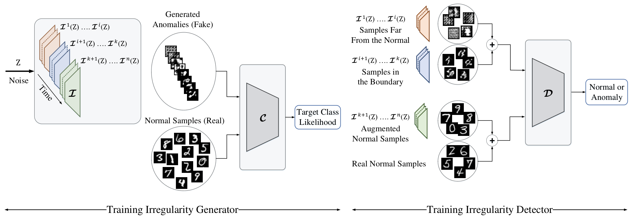
acts as an irregularity generator, while it is totally unaware of such samples. The key idea is to train a GAN on normal samples and utilize its generator before the complete convergence. In fact, generated irregular data should have some deviation from normal instances. Generated irregularities by alongside the available normal samples, form an informative training set for optimizing the parameters of a Convolutional Neural Network (CNN) like to distinguish between normal and anomalous samples. A sketch of our proposed method is shown in Fig. 2. The detailed information of , and is described in the following sections.
3.1 : rregularity Generator Network
GAN is a well-known framework to implicitly learn the real data distribution. Furthermore, it can effectively generate samples following the learned distribution. Generally, a GAN is composed of two neural networks, Generator (G) and Discriminator (D). G tends to generate samples similar to the real ones, while the D attempts to correctly distinguish between generated (fake) and real (target class) data. These two networks are trained adversarially and in competing with each other through a min-max objective function. There are several efficient methods which take advantage of GANs to learn the distribution of their target class and use D as an irregularity detector ravanbakhsh2019training; sabokrou2018adversarially; mohammadi2019end; ahmadi2019generative. Inspired by these works, but from a different point of view, we exploit GANs to learn an efficient deep neural network in presence of samples from both normal and outlier classes.
As explained previously, owing to the high diversity of samples belonging to the outlier class, researchers are unwilling to model and also learn such classes. Thus, they confine the learning process to only the target class. On the contrary, we aim to generate samples from the unseen class to solve the OCC problem as a simple binary classification task.
is tailored for generating samples from the the unseen class data. This network receives a random noise vector sampled from Gaussian distribution, i.e., , as input, and then maps it to an image. Such networks can easily generate samples which do not follow the target class distribution even with no need for the training procedure and only based on randomly initialized parameters. By considering and as the unseen and target class respectively, the number of unseen samples is very larger than target class data, i.e., ( counts the number of samples). Consequently, , as a randomly generated sample by belongs to the unseen class with high probability (i.e., ). Generated instances in this way, is not sufficiently informative to use as training set for a classifier because: (1) generated samples are not semantically similar to the real images, and (2) they are very different from the target class while for a binary classification, samples that are near the boundary of two classes (e.g., support vectors in SVM) are essential. To this end, we train on samples from the target class to play the role of G network of GANs. and are jointly and adversarially trained. After the training process, generates samples following the target class distribution, i.e., .
network gradually learns the distribution of the target class. Let be the learned distribution by in epoch. In the learning period, gradually approaches . Finally, in the optimum point, i.e., , meets . During the training of network, the learned distributions, from to , and generated samples by can be interpreted as follows:
- •
, As explained earlier, we expect that a sample generated by a random CNN, does not comply with the distribution of the target class. Accordingly, samples like are very far from normal instances.
- •
For , . In other words, it is obvious that more training leads to better understanding of real data distribution.
- •
We observe that, For close to , the KL(, where KL and are the distance between two distributions and a small number close to zero, respectively. In this case, generates samples, which in term of texture, are very similar to the target class data, but semantically are completely different. We investigate that such instances can be considered as the boundary outlier class data enclosing the target class samples.
In summary, we save the parameters of after each epoch. Therefore, we have a set of generator networks, i.e., ). can be used for generating: (1) random samples which are very far from the target class data, (2) outliers surrounding the normal samples, i.e., instances which are in the boundary of the target and the outlier class, and (3) samples following the target class distribution. (1) and (2) are used for generating outlier samples, while (3) is appropriate for augmenting the target class data. By generating outliers, the OCC task turns into a binary classification problem. Note that is a CNN which its details is represented in Fig. 3.

3.2 : etector Network
network is a classifier for distinguishing the normal samples from the simulated anomalies. After the training process (see Section 3.3), there are sufficiently available data to train a binary classifier. shows the samples generated by network where . Here, is the number of selected model extracted from the training procedure of the GAN and represents the number of samples generated by each of selected models. Additionally, is the available normal data. Finally, a fully connected neural network, which ends with a softmax layer as a binary classifier, can be trained on and in order to properly perform the anomaly detection task. The softmax layer outputs two scalar values indicating what class (target or outlier) the processed sample belongs to. The overall scheme of network is represented in Fig. 3. is learned by optimizing the Equ. 1.
| (1) |
Where y is the label (1 for anomaly and 0 for normal) and p(y) is the predicted probability of a sample being abnormal for all data.
3.3 Training: and
As explained previously, Goodfellow et al. goodfellow2014generative has introduced an efficient way for adversarial learning of two different neural networks, G and D , called GAN. GANs aim to generate samples that follow the real data distribution through the adversarial training of two networks. G learns to map a latent space like sampled from a specific distribution, i.e., , to a real data distribution (referred to as ). D is trained by maximizing the probability of assigning the correct label to both the actual data and the fake data from G, while G is simultaneously trained to minimize . In other words, G and D play the following two-players mini-max game:
| (2) |
GANs suffer from the fundamental problems which can also cause difficulties for our algorithm: (1) GANs are not stable and the model may never converge. In fact, the G loss does not indicate that an abnormal sample is far form the normal ones or it resides in the boundary, (2) the behavior of GANs is not interpretative. Generally, we expect that decreasing the loss of G results in increasing the quality of the generated images. But, contrary to our expectation, it may not happen in practice, and (3) mode collapse is common for the conventional GANs.
To avoid that defects of the conventional GANs negatively affect our work, Wasserstein GAN (WGAN) is utilized instead. The discriminator of WGANs are broadly known as ritic (). network of WGAN is similar to G network of GAN, but the sigmoid function is eliminated. In WGAN, network outputs a scalar score rather than a probability. This score can be interpreted as how real the input images are. In other words, it measures how good a state (the input) is. network is optimized based on the Equ. 3.
| (3) |
In GAN, the loss measures how well it fools D networks rather than a measure of the image quality. The G loss in GAN does not drop even the image quality improves. Hence, its value does not properly reflect the progress. Instead, we need to save the testing images and evaluate it visually. On the contrary, the loss function of WGAN indicates the image quality which is more desirable and it is calculated based on the Equ. 4.
| (4) |
The loss of WGAN is much more stable than GAN loss enabling us to continue learning without experiencing the drop in accuracy. During training, models have been saved for each epoch. Accordingly, we have different models after epochs.
Selecting networks of saved models as irregularly generators can be done in two ways: (1) using validation set including both normal and anomalous data, and (2) by analyzing network loss. In reality, there are not any samples from outlier class. Hence, using validation samples is not feasible, i.e., this approach is flatly contradict our primary assumption. To follow the second solution, the irregularity networks are selected as follows:
Where, (in our case h=5), is a generated irregularity and is the loss value of in epoch. With respect to Fig. 4, and . Fig 4 shows the relation between the loss of in training duration and the role of network.
Hereupon, the classifier network should learn the distribution of normal samples to be able to effectively separate normal and abnormal instances from each other. Having selected the models for , each of models can generate samples. In this case, we have samples in addition to normal data. For the classifier network, normal samples are considered as real data belonging to the target class while anomalous samples fall into the outlier class because they are considered as the fake data.
3.4 Irregularity Detection
We aim to proposed an end-to-end neural network to detect irregular samples. Accordingly, as explained previously, merely network plays the role of anomaly detector in videos and outlier detector in images. The binary classification problem, which is the converted version of the OCC task in our case, can be simply formulated as:
Where is a predetermined threshold (in our case is equal to ).
4 Experimental Results

We comprehensively evaluate our proposed solution, i.e., G2D, on different datasets. The experimental results alongside an in-depth analysis are presented in this section. Obtained results confirms the superiority of G2D compared to the other baseline and state-of-the-art methods. To show the generality and applicability of the proposed framework for a variety of tasks, we test it for detecting: (1) outlier images, and (2) video anomalies.
4.1 Implementation Details
We implement G2D using PyTorch framework and Python ran on a 64-bit Ubuntu 18.04 LTS system with an Intel corei7 3.80GHz processor, 16 GB RAM and NVIDIA GTX 1080 GPU. We use Adam as the optimizer. The learning rate of and are the same and equal to 0.0001 with 0.5 as Beta1, 0.999 as Beta2 and a batch size of 64. For network, optimizer is SGD and learning rate is equal to 0.01. Also, momentum is equal to 0.9 with a batch size of 32. We use negative log likelihood function as the loss function for network. The detailed structures of and is explained in Sections 3.1 and 3.2, respectively. These structures are kept fixed for different tasks.
4.2 Datasets
UCSD: This dataset mahadevan2010anomaly is composed of two subsets, Ped1 and Ped2 which are derived from two different outdoor scenes recorded by a static camera with 10 fps. The resolutions of Ped1 and Ped2 are 158234 and 240360, respectively. Since the dominant mobile objects are pedestrians in these scenes, the rest objects (e.g., cars, skateboarders, wheelchairs or bicycles) are considered as anomalies. Our proposed algorithm has been evaluated on Ped2.
MNIST: This dataset lecun2010mnist consists of 60,000 handwritten digits from “0” to “9”. Each of digit categories is considered as the target class, i.e., inlier, and the outliers are simulated by randomly sampling images from the other categories with the proportion of 10% to 50%. This process has been repeated for all of digit categories.
Caltech-256: This dataset griffin2007caltech includes 256 object categories and 30,607 images in total. Each category contains at least 80 images. Analogous with the previous works sabokrou2018adversarially, the procedure is repeated three times. We have used which are randomly chosen categories as inliers, i.e., target class data. The first 150 images of each category is opted in case that the category has more than 150 images. A certain number of outliers are randomly selected from the “clutter” category. Each of conducted experiments includes exactly 50% outliers.
4.3 Video Anomaly Detection
Visual analysis of unusual and rare events has been drawn the attention of many researchers in computer vision communities. The complexity of the video processing poses even more challenges for detecting anomalous events or novelty compared to outlier detection in image processing. G2D is evaluated on a widely-used and popular dataset, USCD mahadevan2010anomaly Ped2. The results are reported based on frame-level basis.
Results on UCSD Ped2: In this experiment, each frame is divided into 2D patches of size 3030 with the overlap of 5. As explained in Section 3.3, network generates a set of irregular samples with the same size of normal patches. In this way, network is trained on both generated irregular and available normal patches as a binary classifier. In the state of test, is able to detect whether the extracted patches of a frame is abnormal or not.
The comparison is made based on a frame-level Equal Error Rate (EER). To this end, detecting a pixel of a frame as anomaly leads to considering the whole frame as an abnormal sample. Table 1 represents the results obtained from the conducted experiments. As it is clear, we have attained comparable and even better result to the other state-of-the-art methods while our work is general with no further tuning to the video based tasks or any other specific applications. Note that G2D treats video as images, i.e., unlike the other approaches (especially Deep-Cascade sabokrou2017deep and Deep-Anomaly sabokrou2018deep) benefited from both spatial and temporal complex features, our proposed method operates on a patches extracted from the spatial features of the frames.
| Method | EER | Method | EER | |
| MPCCA kim2009observe | 30% | RE sabokrou2016video | 15% | |
| Sabokrou et al.sabokrou2018deep | 16% | Ravanbakhsh et al. ravanbakhsh2019training | 13% | |
| MDT mahadevan2010anomaly | 24% | Ravanbakhsh et al. ravanbakhsh2017abnormal | 14% | |
| Li et al. li2013anomaly | 18.5% | Deep-Anomalysabokrou2018deep | 13% | |
| Dan Xu et al. xu2014video | 20% | Deep-cascade sabokrou2019self | 9% | |
| AVIDsabokrou2018avid | 14% | NRE sabokrou2019self | 14% | |
| ALOCC sabokrou2018adversarially | 13% | Ours (G2D) | 11% |
4.4 Image Outlier Detection
If machine learning based methods fail in dealing with processing the data contaminated by noise and irregularities, they experience a considerable drop in performance. The necessity of providing a proper solution to cope with this problem is inevitable because outliers are very common in realistic vision-based training sets. we evaluate the performance of G2D using MNIST and Caltech datasets.
Results on MNIST: and networks are adversarially and jointly trained on normal samples. Similar to the previous experiments, outlier samples simultaneously are generated and network is trained on normal and generated abnormal samples. We report the performance of our method based on -score measure against the percentage of outlier instances. Figure 5 confirm that G2D has a better performance, in terms of -score, compared to the other state-of-the-art methods. Also, as can be seen, G2D is insensitive to change of outlier portion. The other baseline solutions have a reference model which learns the distribution of normal data. Accordingly, they are able to effectively detect normal sample while facing unusual events cause a sharp drop in their performance. Hence, when outliers form 10% of the total data, all of the methods performs well. However, with the increase of outliers in number, -score has declined. On the other hand, G2D knows the concept of both normal and abnormal data (generated anomalous samples) leading to the higher precision for detecting anomalies and operates more robust. Therefore, the growth of outliers has a negligible effect on the performance of our proposed method and thus it does not experience a noticeable drop in -score measure.
| R-graph you2017provable | REAPER lerman2015robust | OutlierPursuit xu2010robust | LRR liu2010robust | SSGAN kimura2018semi | ALOCC sabokrou2018adversarially | Ours (G2D) | |
| AUC | 0.948 | 0.816 | 0.837 | 0.907 | - | 0.942 | 0.957 |
| 0.914 | 0.808 | 0.823 | 0.893 | 0.977 | 0.928 | 0.945 | |
| AUC | 0.29 | 0.796 | 0.788 | 0.479 | - | 0.938 | 0.951 |
| 0.880 | 0.784 | 0.779 | 0.671 | 0.963 | 0.913 | 0.922 | |
| AUC | 0.913 | 0.657 | 0.629 | 0.337 | - | 0.923 | 0.939 |
| 0.858 | 0.716 | 0.711 | 0.667 | 0.945 | 0.905 | 0.913 |
Results on Caltech-256: We compare our work with other six methods therein designed specifically for outlier detection, including R-graph you2017provable, REAPER lerman2015robust, OutlierPursuit xu2010robust, LRR liu2010robust, SSGAN kimura2018semi and ALOCC sabokrou2018adversarially. The performance metrics of this experiment are -score and the Area Under the Curve (AUC). Results listed in the Table 2 confirm G2D performs at least as good as the other solutions, whereas it outperforms them in many cases.
4.5 Complexity
In our method, irregularity detection is only performed by network. Hence, there is an end-to-end architecture which is capable of processing an image or video with a lower complexity than the other GAN-based state-of-the-art methods such as AVIDsabokrou2018avid or ALOCCsabokrou2018adversarially. Irregularity detection is properly done if a sample processed by two complicated neural networks either for ALOCC or AVD. Otherwise, these algorithms are not able to attain high accuracy. For more details, ALOCC utilized both G network, which includes an encoder-decoder neural network, and D network of a pre-trained GAN to achieve better results.
5 Discussion
In this section, the significant issues and the way of dealing with them by our proposed method, i.e., G2D, are thoroughly investigated.
Weak supervision: G2D is an unsupervised method even though knowing that there is not any irregular samples among the training data can be considered as a weak supervision. In reality, abnormal data are rare and broadly form just a little portion of all samples. Accordingly, the existence of a few number of anomalous instances among the normal data is not problematic in case of considering all the available data as normal.
Generality: G2D is a general purpose framework for the OCC task which can easily fit to various range of problems (see Section 3). However, we have achieved comparable and even better results than the other state-of-the-arts (see Section 4). Obviously, If we customize our algorithm, e.g., by some modifications in the size and the order of convolutional layers, for a specific-purpose application, the final performance improves.
Convenience of implementation: G2D is easily implementable forming one of the most important of our contributions. Generally, GAN-based approaches suffer form finding the optimum point for stopping the training process of its two joint neural networks, G and D. In fact, determining a suitable moment in which the discriminator learns the distribution of the normal data is very challenging. On the contrary, our method does not get involved with this burdensome task because we utilized non-optimal trained models for simulationary generating abnormal samples.
Normal data augmentation: As discussed in Section 3.1, all of the models are saved during training. Samples can be generated by the trained models fall into three categories: (1) far from the target class, (2) near to the boundary, and (3) semantically similar to normal samples. Having trained network, models belonging to the third category are appropriate for generating samples following the concept of normal data and very similar to them. Therefore, we can use our algorithm for augmenting normal class. This feature is very useful especially when the normal instances are not sufficient.
False positive rate reduction: The majority of the proposed solution for the OCC task, like anomaly detection, suffer from high false positive rate. This difficulty is mainly caused by the samples resides in the boundary between normal and anomalous data. Lim et al. lim2018doping attempted to solve this problem by generating normal data in the boundary. Also, we are able to solve this problem by carefully generating abnormal instances. However, producing anomalies mistakenly does not help. In order to gain better performance in this regard, we can check the quality of simulated anomalies. High quality of the generated samples is an indicator that the model is very close to a suitable boundary which can effectively distinguish between normal and abnormal instances. Note that reducing the false positive rate is just one of the application of our work while it is the main contribution of lim2018doping.
6 Conclusion
In this paper we propose a general purpose framework for irregularity detection. Firstly, two networks are unsupervisedly and adversarially trained on just normal samples aiming to generate irregular data. Afterward, a deep neural network as a binary classifier learns the simultaneously generated anomalies along with the available normal instances. Result have confirmed that our proposed method, i.e., G2D, can accurately detect irregularities while it is totally unaware of abnormal class data.
Acknowledgement
This research was in part supported by a grant from IPM (No. CS1396-5-01).
References
- (1) Ehsan Adeli, Kim-Han Thung, Le An, Feng Shi, and Dinggang Shen. Robust feature-sample linear discriminant analysis for brain disorders diagnosis. In Advances in Neural Information Processing Systems, pages 658–666, 2015.
- (2) Milad Ahmadi, Mohammad Sabokrou, Mahmood Fathy, Reza Berangi, and Ehsan Adeli. Generative adversarial irregularity detection in mammography images. In International Workshop on PRedictive Intelligence In MEdicine, pages 94–104. Springer, 2019.
- (3) Borislav Antić and Björn Ommer. Video parsing for abnormality detection. In Computer Vision (ICCV), 2011 IEEE International Conference on, pages 2415–2422. IEEE, 2011.
- (4) Marco Bertini, Alberto Del Bimbo, and Lorenzo Seidenari. Multi-scale and real-time non-parametric approach for anomaly detection and localization. Computer Vision and Image Understanding, 116(3):320–329, 2012.
- (5) Oren Boiman and Michal Irani. Detecting irregularities in images and in video. International journal of computer vision, 74(1):17–31, 2007.
- (6) Markus M Breunig, Hans-Peter Kriegel, Raymond T Ng, and Jörg Sander. Lof: identifying density-based local outliers. In ACM sigmod record, volume 29, pages 93–104. ACM, 2000.
- (7) Yang Cong, Junsong Yuan, and Ji Liu. Sparse reconstruction cost for abnormal event detection. In Computer Vision and Pattern Recognition (CVPR), 2011 IEEE Conference on, pages 3449–3456. IEEE, 2011.
- (8) Eleazar Eskin. Anomaly detection over noisy data using learned probability distributions. In In Proceedings of the International Conference on Machine Learning. Citeseer, 2000.
- (9) Ian Goodfellow, Jean Pouget-Abadie, Mehdi Mirza, Bing Xu, David Warde-Farley, Sherjil Ozair, Aaron Courville, and Yoshua Bengio. Generative adversarial nets. In Advances in neural information processing systems, pages 2672–2680, 2014.
- (10) Gregory Griffin, Alex Holub, and Pietro Perona. Caltech-256 object category dataset. 2007.
- (11) Jaechul Kim and Kristen Grauman. Observe locally, infer globally: a space-time mrf for detecting abnormal activities with incremental updates. In 2009 IEEE Conference on Computer Vision and Pattern Recognition (CVPR), pages 2921–2928. IEEE, 2009.
- (12) Masanari Kimura and Takashi Yanagihara. Semi-supervised anomaly detection using gans for visual inspection in noisy training data. arXiv preprint arXiv:1807.01136, 2018.
- (13) Yann LeCun, Corinna Cortes, and Christopher JC Burges. Mnist handwritten digit database. AT&T Labs [Online]. Available: http://yann. lecun. com/exdb/mnist, 2, 2010.
- (14) Gilad Lerman, Michael B McCoy, Joel A Tropp, and Teng Zhang. Robust computation of linear models by convex relaxation. Foundations of Computational Mathematics, 15(2):363–410, 2015.
- (15) Weixin Li, Vijay Mahadevan, and Nuno Vasconcelos. Anomaly detection and localization in crowded scenes. IEEE transactions on pattern analysis and machine intelligence, 36(1):18–32, 2013.
- (16) Swee Kiat Lim, Yi Loo, Ngoc-Trung Tran, Ngai-Man Cheung, Gemma Roig, and Yuval Elovici. Doping: Generative data augmentation for unsupervised anomaly detection with gan. In 2018 IEEE International Conference on Data Mining (ICDM), pages 1122–1127. IEEE, 2018.
- (17) Guangcan Liu, Zhouchen Lin, and Yong Yu. Robust subspace segmentation by low-rank representation. In Proceedings of the 27th international conference on machine learning (ICML-10), pages 663–670, 2010.
- (18) Vijay Mahadevan, Weixin Li, Viral Bhalodia, and Nuno Vasconcelos. Anomaly detection in crowded scenes. In 2010 IEEE Computer Society Conference on Computer Vision and Pattern Recognition (CVPR), pages 1975–1981. IEEE, 2010.
- (19) Markos Markou and Sameer Singh. Novelty detection: a review—part 1: statistical approaches. Signal processing, 83(12):2481–2497, 2003.
- (20) Bahram Mohammadi and Mohammad Sabokrou. End-to-end adversarial learning for intrusion detection in computer networks. In 2019 IEEE 44th Conference on Local Computer Networks (LCN), pages 270–273, 2019.
- (21) Brendan Tran Morris and Mohan M Trivedi. Trajectory learning for activity understanding: Unsupervised, multilevel, and long-term adaptive approach. IEEE transactions on pattern analysis and machine intelligence, 33(11):2287–2301, 2011.
- (22) Trong-Nguyen Nguyen and Jean Meunier. Anomaly detection in video sequence with appearance-motion correspondence. In Proceedings of the IEEE International Conference on Computer Vision, pages 1273–1283, 2019.
- (23) Pramuditha Perera, Ramesh Nallapati, and Bing Xiang. Ocgan: One-class novelty detection using gans with constrained latent representations. In Proceedings of the IEEE Conference on Computer Vision and Pattern Recognition, pages 2898–2906, 2019.
- (24) Mostafa Rahmani and George Atia. Coherence pursuit: Fast, simple, and robust principal component analysis. arXiv preprint arXiv:1609.04789, 2016.
- (25) Mahdyar Ravanbakhsh, Moin Nabi, Enver Sangineto, Lucio Marcenaro, Carlo Regazzoni, and Nicu Sebe. Abnormal event detection in videos using generative adversarial nets. In 2017 IEEE International Conference on Image Processing (ICIP), pages 1577–1581. IEEE, 2017.
- (26) Mahdyar Ravanbakhsh, Enver Sangineto, Moin Nabi, and Nicu Sebe. Training adversarial discriminators for cross-channel abnormal event detection in crowds. In 2019 IEEE Winter Conference on Applications of Computer Vision (WACV), pages 1896–1904. IEEE, 2019.
- (27) Mohammad Sabokrou, Mahmood Fathy, and Mojtaba Hoseini. Video anomaly detection and localisation based on the sparsity and reconstruction error of auto-encoder. Electronics Letters, 52(13):1122–1124, 2016.
- (28) Mohammad Sabokrou, Mahmood Fathy, Mojtaba Hoseini, and Reinhard Klette. Real-time anomaly detection and localization in crowded scenes. In Proceedings of the IEEE CVPR Workshops, pages 56–62, 2015.
- (29) Mohammad Sabokrou, Mahmood Fathy, Guoying Zhao, and Ehsan Adeli. Deep end-to-end one-class classifier. IEEE Transactions on Neural Networks and Learning Systems, 2020.
- (30) Mohammad Sabokrou, Mohsen Fayyaz, Mahmood Fathy, and Reinhard Klette. Deep-cascade: Cascading 3d deep neural networks for fast anomaly detection and localization in crowded scenes. IEEE Transactions on Image Processing, 26(4):1992–2004, 2017.
- (31) Mohammad Sabokrou, Mohsen Fayyaz, Mahmood Fathy, Zahra Moayed, and Reinhard Klette. Deep-anomaly: Fully convolutional neural network for fast anomaly detection in crowded scenes. Computer Vision and Image Understanding, 172:88–97, 2018.
- (32) Mohammad Sabokrou, Mohammad Khalooei, and Ehsan Adeli. Self-supervised representation learning via neighborhood-relational encoding. International Conference on Computer Vision (ICCV), 2019.
- (33) Mohammad Sabokrou, Mohammad Khalooei, Mahmood Fathy, and Ehsan Adeli. Adversarially learned one-class classifier for novelty detection. In Proceedings of the IEEE Conference on Computer Vision and Pattern Recognition (CVPR), pages 3379–3388, 2018.
- (34) Mohammad Sabokrou, Masoud Pourreza, Mohsen Fayyaz, Rahim Entezari, Mahmood Fathy, Jürgen Gall, and Ehsan Adeli. Avid: adversarial visual irregularity detection. In Asian Conference on Computer Vision, pages 488–505. Springer, 2018.
- (35) Kuldeep Singh, Shantanu Rajora, Dinesh Kumar Vishwakarma, Gaurav Tripathi, Sandeep Kumar, and Gurjit Singh Walia. Crowd anomaly detection using aggregation of ensembles of fine-tuned convnets. Neurocomputing, 371:188 – 198, 2020.
- (36) Yao Tang, Lin Zhao, Shanshan Zhang, Chen Gong, Guangyu Li, and Jian Yang. Integrating prediction and reconstruction for anomaly detection. Pattern Recognition Letters, 129:123 – 130, 2020.
- (37) Yan Xia, Xudong Cao, Fang Wen, Gang Hua, and Jian Sun. Learning discriminative reconstructions for unsupervised outlier removal. In Proceedings of the IEEE International Conference on Computer Vision, pages 1511–1519, 2015.
- (38) Dan Xu, Elisa Ricci, Yan Yan, Jingkuan Song, and Nicu Sebe. Learning deep representations of appearance and motion for anomalous event detection. arXiv preprint arXiv:1510.01553, 2015.
- (39) Dan Xu, Rui Song, Xinyu Wu, Nannan Li, Wei Feng, and Huihuan Qian. Video anomaly detection based on a hierarchical activity discovery within spatio-temporal contexts. Neurocomputing, 143:144–152, 2014.
- (40) Huan Xu, Constantine Caramanis, and Sujay Sanghavi. Robust pca via outlier pursuit. In Advances in Neural Information Processing Systems, pages 2496–2504, 2010.
- (41) Kenji Yamanishi, Jun-Ichi Takeuchi, Graham Williams, and Peter Milne. On-line unsupervised outlier detection using finite mixtures with discounting learning algorithms. Data Mining and Knowledge Discovery, 8(3):275–300, 2004.
- (42) Chong You, Daniel P Robinson, and René Vidal. Provable self-representation based outlier detection in a union of subspaces. In Proceedings of the IEEE Conference on Computer Vision and Pattern Recognition, pages 3395–3404, 2017.