Physical Properties of a Regular Rotating Black Hole:
Thermodynamics, Stability, Quasinormal Modes
Abstract
Respecting the angular momentum conservation of torque-free systems, it is natural to consider rotating solutions of massive objects. Besides that, motivated by the realistic astrophysical black holes that rotate, we use the Newman-Janis formalism to construct a regular rotating black hole. We start with a nonlinearly charged regular static black hole in the framework of the standard general relativity and then obtain the associated rotating solution through such a formalism. We investigate the geometrical properties of the metric by studying the boundary of ergosphere. We also analyze thermodynamic properties of the solution in AdS spacetime and examine thermal stability and possible phase transition. In addition, we perturb the black hole by using of a real massless scalar field as a probe to investigate its dynamic stability. We obtain an analytic expression for the real and imaginary parts of the quasinormal frequencies. Finally, we look for a connection between the quasinormal frequencies and the properties of the photon sphere in the eikonal limit.
I Introduction
One of the main open questions in theoretical physics is the existence of singularity in different theories. From the gravitational point of view, there might be something mysterious about the spacetime singularity. Thus, investigation of such a pathology is a hot topic, either in physical and mathematical communities or in philosophical circle.
The Einstein general relativity not only admits different solutions including singularity, but expresses that such a singularity may be unavoidable a real-world scenario. For this reason, one has to perceive the nature of singularity to understand the nature of singular spacetimes. Nonetheless, since the general relativity could not describe the nature and physical properties of the spacetime singularity, one may look for alternative viewpoint. The possibility of constructing a nonsingular (regular) spacetime might be potentially important implication for avoiding the breakdown of physical laws near the singularity, a region with extreme curvature and vanishing volume. In addition, there is as yet no a consistent theory of quantum gravity and some scientists believe that the singularity would not occur in such a theory. Fortunately, the Einstein general relativity allows some regular solutions without curvature singularity which contain at most coordinate singularity Bardeen. It is worth mentioning that such regular black holes are not vacuum solutions of the Einstein field equations. These regular solutions often include a special class of nonlinear electrodynamics violating energy conditions in the vicinity of the black hole Ayon-Beato1-Sajadi:2017glu. Till date there has been a lot of significant work in regular solutions of gravitating systems Bronnikov:2001tv-Dymnikova:1992ux.
On the other hand, according to the published results of the gravitational wave observatories by the collaborations LIGO and VIRGO LIGO1; LIGO2; LIGO3 and shadow of black hole by Event Horizon Telescope Akiyama:2019cqa-Akiyama:2019bqs, one finds that the astrophysical black holes are not static and spherically symmetric, but asymmetric due to they have rotation. In other words, one of the most realistic features of relativistic black holes is that they have angular momentum in a stationary manner. Hence, in order to have a pragmatic black hole solution, one has to consider rotating spacetime. However, introducing a new rotating black hole solution, directly, is a nontrivial task as it turns out to be a rather long process to obtain the Kerr solution. However, one may use the Newman-Janis algorithm to convert static solutions to rotating ones Newman-Modesto. A special solution of the Kerr black hole in the presence of electromagnetic field is obtained in Liao2017. Phase transition of the Kerr-Newman-AdS black hole with a model of dark energy is discussed in Jafarzade2017 and its extension to nonlinear magnetic charge in Ndongmo2019. The astrophysical aspects of rotating black holes, such as shadow images and the geodetic precession frequency, have already been studied in Haroon2019; Rizwan2019. Besides that, other physical properties of rotation black holes, in particular thermodynamic behavior and photon sphere are of interest.
Taking into account the quantum effects near a black hole, one has to regard it as a thermodynamical entity with a temperature and an entropy. Such a statement help us to understand a deep connection among three interesting theories; general relativity, quantum field theory and thermodynamics. In other words, the black hole thermodynamics can be used as a bridge to connect two apparently independent theories, general relativity and quantum field theory. Black hole thermodynamics began, seriously, with the pioneering works of Hawking and Beckenstein, and has recently become very fascinating in the extended phase space by considering the cosmological constant as a thermodynamic quantity. Taking a dynamical cosmological constant into account, the consistent first law of black hole thermodynamics and the associated Smarr relation are modified by including a term. Comparing such a modified first law of black hole thermodynamics with that of everyday system, we find that in this representation, the mass of the black hole is considered as the enthalpy of the system instead of the internal energy kastor09-kubiznak14. Exploring the phase transition and critical behavior of the black hole solutions in the extended phase space is another interesting issue which is reported for different gravitating systems kubiznak12; Gunasekaran-Hendi. Thermal stability of a black hole plays an important role in exploring its behavior near the equilibrium. It is notable that a thermally stable black hole has a non-negative heat capacity.
In addition to thermal stability criteria, one has to examine dynamical stability of black holes under perturbations of the geometry and matter fields. The robustness check of black holes against small perturbations is sufficiently strong to veto some mathematical black holes. Regarding a perturbative black hole, one may observe some oscillated behavior, named as quasinormal modes (QNMs) which are related to some quasinormal frequencies (QNFs). It is shown that QNMs are the intrinsic imprints of the black hole response to external perturbations which means that such QNMs are independent of initial perturbations. Authors of Refs. Nollert1993; Hod1998 show that the asymptotic behavior of QNMs is related to the quantum nature of gravitation. It is also reported that for AdS black holes, the imaginary parts of QNFs are corresponding to the perturbations damping of a thermal state in the conformal field theory Horowitz2000; Cardoso2001. So, the investigation of QNMs help us to find the features of compact objects, the evolution of fields and also the properties of spacetime Kokkotas1999; Berti2009; Konoplya2011.
There are several approaches to the study black hole’s QNMs. Ferrari and Mashhoon vf, working on the potential barrier in the effective one-dimensional Schrodinger equation and obtain simple exact solutions. Such a barrier is related to the photon sphere of the black hole yd. We should note that QNMs of regular black holes have been studied before sf-scu. The behavior of QNMs at the thermodynamics phase transitions has been studied in Konoplya:2017zwo; Sajadi:2019hzo. Moreover, the relation between the QNFs and the thermodynamical quantities at eikonal limit for static solution Hod:1998vk and for rotating one Musiri:2003ed has been studied. Cardoso et al. Cardoso:2008bp showed that the real part of the QNMs is related to the angular velocity of the last circular null geodesic while Stefanov et al. Stefanov:2010xz found a connection between black hole’s QNMs in the eikonal limit and lensing in the strong deflection limit. Furthermore, in Ref. Jusufi:2019ltj the connection between the QNMs and the shadow radius for static black hole and recently for rotating one Jusufi:2020dhz has been obtained. In this work, we use the Newman-Janis formalism to obtain a regular rotating black hole solution. We also study the thermodynamic and phase transition of such a rotating solution in the extended phase space by using of standard approach. In addition, we study the stability of the black hole against perturbation of spacetime and look for the QNMs cv; sc.
The paper is organized as follows. In Sec. II, we study the geometric properties of an interesting class of regular rotating black hole. We study the thermodynamics of rotating AdS black hole and look for possible phase transition in Sec. III. Section IV is devoted to study the QNMs and their connection to the properties of photon sphere in the eikonal limit. The paper ends with our concluding remarks in Sec. V.
II Regular Rotating Black Hole
The dimensional action governing nonlinearly charged black holes in the presence of a negative cosmological constant is given by
| (1) |
in which is the determinant of the metric tensor, denotes the AdS length related to the negative cosmological constant, is the Ricci scalar and is an arbitrary function of the Maxwell invariant . Applying the variational principle to the action (1), one can show that the field equations are given by
| (2) |
| (3) |
where in the above equations is the Einstein tensor and .
The metric of rotating charged regular black hole in the Boyer-Lindquist
coordinates is obtained as Newman, Dymnikova
| (4) |
where
and the functional form of depends on the choice of the EM Lagrangian . Our approximate functional form of is introduced in Balart:2014cga, Ghosh:2014pba as
| (5) |
Here, for the sake of simplicity we have considered above function for . It is worth mentioning that the asymptotic behavior of the metric (4) is in agreement to the Kerr-Newman-AdS black hole.
The radius of the horizon can be obtained from the following
equation
| (6) |
The existence/nonexistence of real positive root of the above equation indicates two scenarios, regular black hole or no-horizon solution. The regular black hole and no-horizon cases may be separated by introducing the extremal horizon of the black hole solution. The extremality condition is defined by the following relation
Regarding , one can obtain
| (7) |
where . It is notable that has a minimum which is corresponding to the extremal configuration for the black hole. So, by taking the derivative of mass with respect to the horizon radius, one can obtain the extremal charge which its maximum value is
| (8) |
For the case of , one can obtain the following relation between the extremal value of quantities
| (9) |
and
| (10) |
where
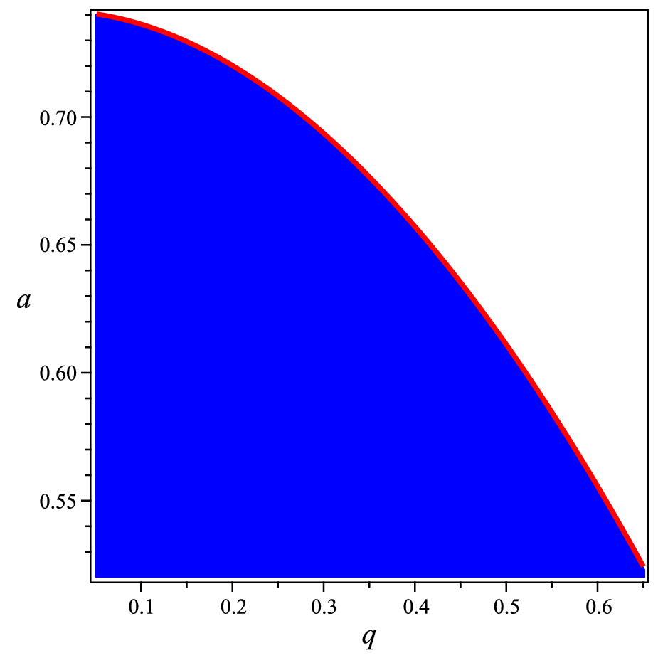
The conditions of having the regular black hole or the no-horizon solution in terms of the free parameters are observed in Fig. 1. In order to have regular black holes, there are upper limits (critical values) on the electric charge and rotation parameter of the metric. At the critical values (the border of the shaded and white regions) there is a minimum horizon which corresponds to the extremal black hole ( plot). The solution has no-horizon in the white region of the plot. In the case of the rotating regular black hole (shaded region of plot), by increasing the rotation parameter the critical value of the electric charge decreases.
Static observers cannot exist everywhere in the spacetime, because the four velocity of static observer finally becomes null. When this occurs the observer cannot remain static and rotate with the black hole.Therefore, the stationary limit surface is described by . Similar to the case of event horizon, one can obtain the conditions for the critical parameter of black hole so that the solutions of () merge to one. The conditions are
| (11) |

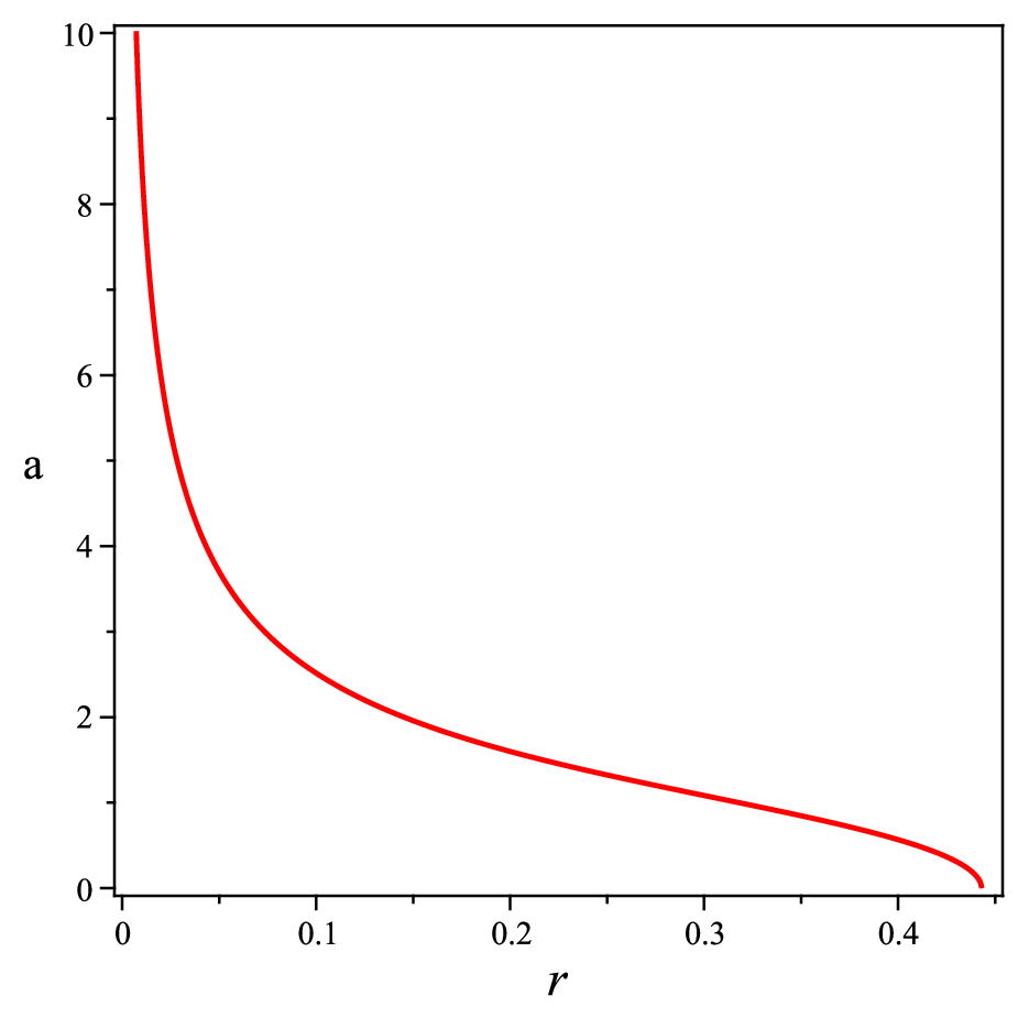
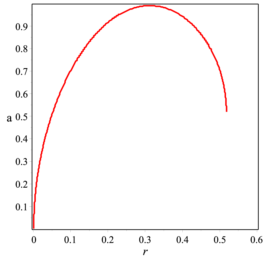
Solving the mentioned conditions, simultaneously, for obtaining and in the case of and plotting them, one can find Fig. 2 and obtain following equations
| (12) |
In the plot, shaded and white plots correspond to the regular black hole with stationary limit surface and without stationary limit surface, respectively. The plot represents the dependence of the radius of the stationary limit surface on .
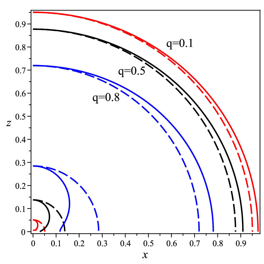

The stationary limit surface does not coincide with the event horizon and is
located outside the horizon. The region between the horizon and the
stationary limit surface is called the ergoregion which is shown in the Fig.
(3). In Fig. (3), size and shape of ergoregion
in the plane, where and , have
been depicted. By increasing and , one can observe the change in the
shape and size of the ergoregion.
We now consider a possible nonlinear source for the metric (4).
The magnetic part of the gauge field () of charged rotating
regular black hole is given by
| (13) |
in which by calculating the electromagnetic field tensor, one obtains
| (14) |
By solving the Einstein tensor for and as independent parameters, one can find
| (15) |
| (16) |
The above definitions for and satisfy all five different Einstein field equations. In the case of , one can recover the expressions presented in Fan:2016hvf. We should note that the total derivative of with respect to is not equal to and their difference in the case of is given as
| (17) |
where its asymptotic limit ()is
| (18) |
In Fig. 4, we have shown in terms of at the equatorial plane of the regular rotating black holes for different values of parameters. According to the Fig. (4), one finds that the inconsistency between and is smaller than . As a result, we find that the metric (4) is a charged rotating solution for the Einstein equation.

III Thermodynamics
In this section, we explore the thermodynamics of the regular rotating-AdS black hole solution (4). In order to investigate the thermodynamic properties of the black hole in extended phase space, we need to obtain some relevant thermodynamic quantities. In the extended phase space, we treat the cosmological constant as a thermodynamic pressure and its conjugate quantity as a thermodynamic volume via dolan10; dolan11; altamirano14:1
| (19) |
where is the horizon area of black hole which is calculated as
| (20) |
and and are, respectively, the mass and the angular momentum of the black hole which can be obtain by using of Altas-Tekin method Altas:2018zjr. Using the Killing vectors and associated with the time translation and rotational invariance, one gets Caldarelli:1999xj
| (21) |
The Hawking temperature for non-extremal case can be obtained by using the surface gravity interpretation
| (22) |
where is the surface gravity. In the case of small and we have
| (23) |
As we know, the Killing vector at the event horizon of the rotating black hole is a null vector, and therefore, we can use
| (24) |
to obtain the angular velocity, , by inserting and from metric (4)
| (25) |
on the horizon , so we obtain following expression for angular velocity
| (26) |
However, we should note that the thermodynamical angular velocity is the differences between the angular velocity measured by the observer at the infinity and the angular velocity at the horizon, yielding
| (27) |
The electric part of vector potential is given as
| (28) |
so, the electrostatic potential of the event horizon with respect to spatial infinity as an electrostatic potential reference is obtained as
| (29) |
where is the null generator of the horizon. By computing the flux of electromagnetic field tensor by using of the standard Gauss’ law, one can obtain the electric charge as follow
| (30) |
where is the dual of the Faraday 2-form. For a black hole embedded in AdS spacetime, employing the relation between the cosmological constant and thermodynamic pressure, would result in the interpretation of the black hole mass as the enthalpy. Using the expressions (21), (30) and (20) for mass, angular momentum, electric charge and entropy, and the fact that , one obtains the enthalpy in terms of thermodynamic quantities as
| (31) |
by using (31), one can determine the temperature, electrostatic potential, volume and angular momentum respectively, as
| (32) |
| (33) |
| (34) |
| (35) |
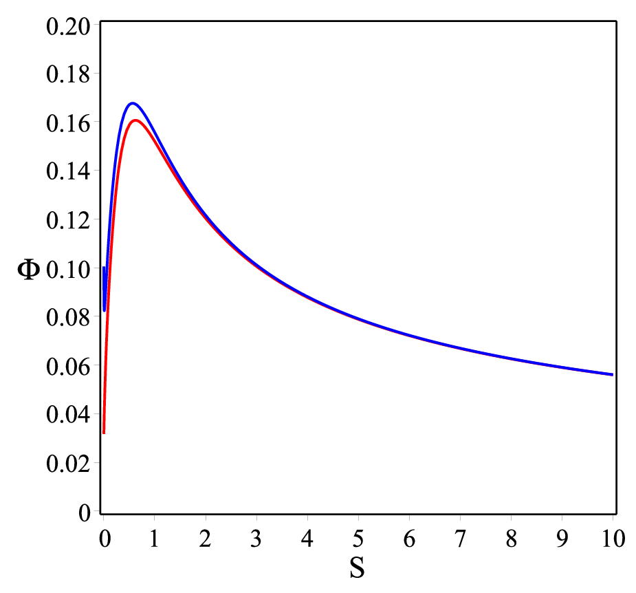
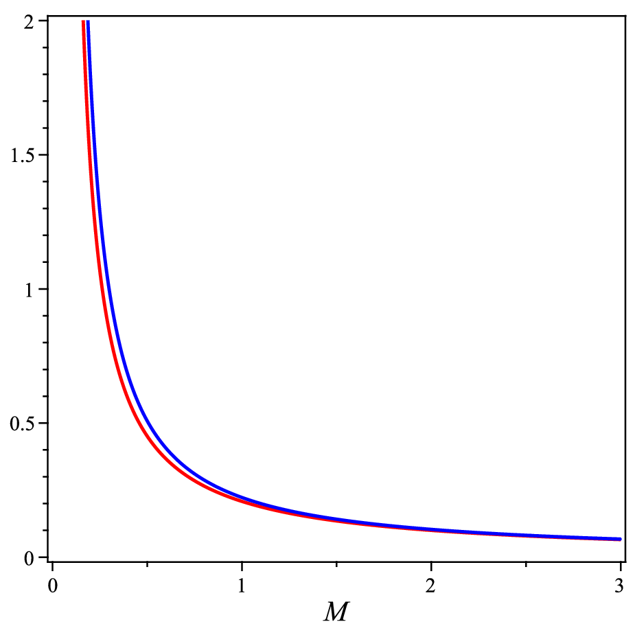
Calculations show that the intensive quantities calculated by Eqs. (32)-(35) coincide with Eqs. (19), (22), (26) and (29) respectively. For instance in Fig. (5), we have done a comparison between relation (33) (red solid line) and (29) (blue solid line).
Thus, these thermodynamic quantities satisfy the first law of black hole thermodynamics in the enthalpy representation
| (36) |
In addition, for the sake of completeness, we calculate the Smarr relation. Using the scaling argument, it should be given as
| (37) |
In figure 6, we have shown the differences between left and right of equation (37). As can be seen, the figure shows the familiar Smarr relation is satisfied.

III.1 Phase transition and stability
Thermodynamic stability tells us how a system in thermodynamic equilibrium responds to fluctuations of thermodynamic parameters. We should distinguish between global and local stability. In global stability, we allow a system in equilibrium with a thermodynamic reservoir to exchange energy with the reservoir. The preferred phase of the system is the one that minimizes the Gibbs free energy. In order to investigate the global stability, we use the following expression for the Gibbs free energy in terms of , and
| (38) |
in which at the large , we have
| (39) |
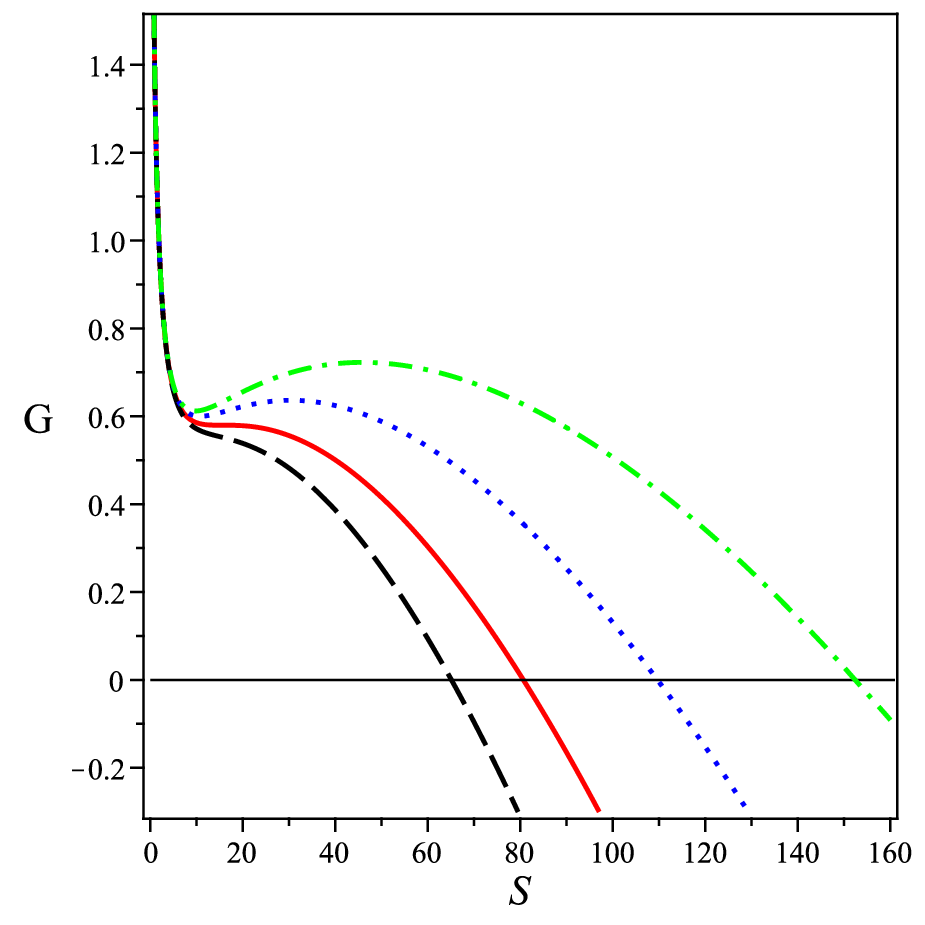
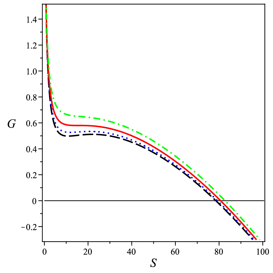
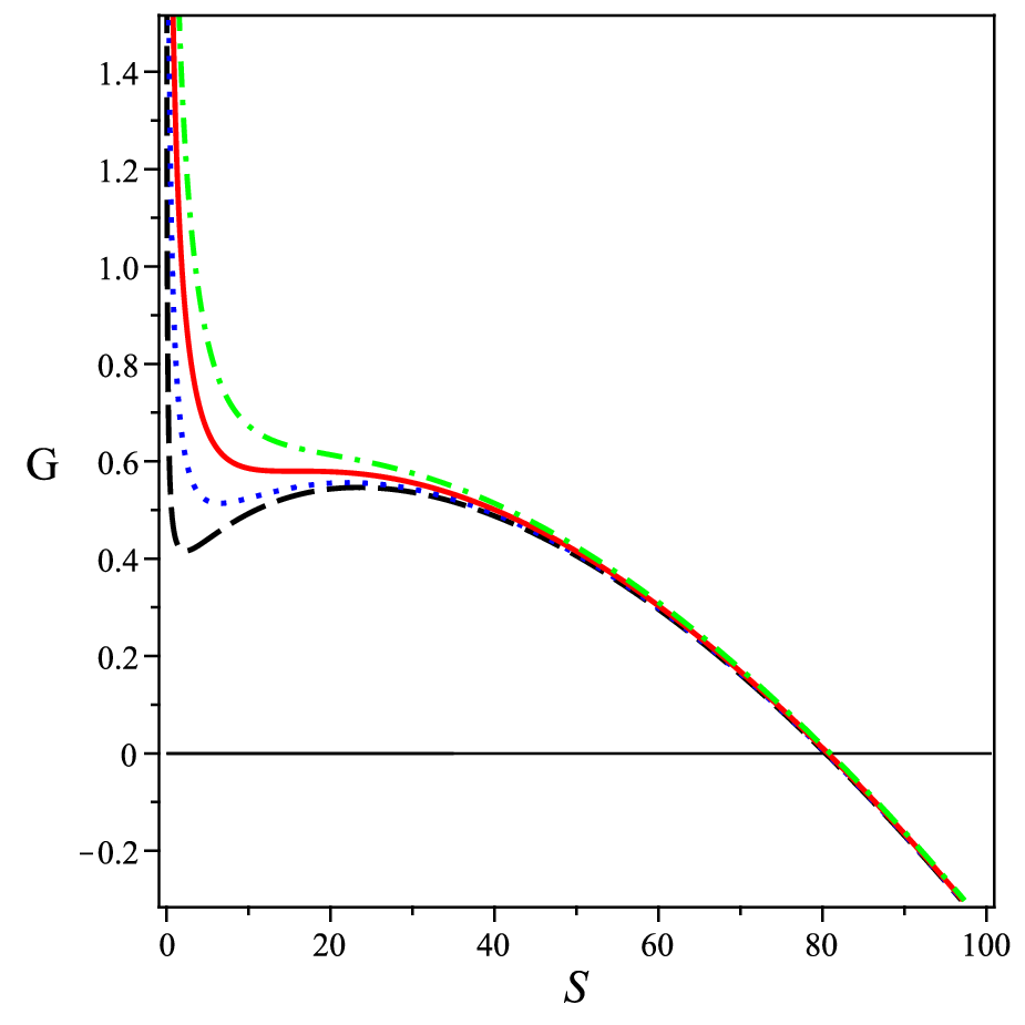
In Fig. (7), we have shown the Gibbs free energy in terms of
entropy. Considering Fig. (7), we find that for
constant and , the Gibbs free energy is a decreasing function of
for both small and large event horizon entropy, while it is an increasing
function for intermediate . This behavior confirms that intermediate
black holes are globally unstable. Since the large black holes have negative
Gibbs free energy, they are more stable than small black holes. Also, Fig. (7) shows that by increasing the pressure the black hole is
more stable. Also, we have shown the behavior of the Gibbs free energy in
terms of for constant pressure and angular momentum in Fig. (7) and for constant pressure and electric charge in Fig. (7). It is obvious that by increasing the angular
momentum and electric charge the black hole is more stable.
On the other hand, local stability is concerned with how the system responds
to small changes in its thermodynamic parameters. In order to study the
thermodynamic stability of the black holes with respect to small variations
of the thermodynamic coordinates, one can investigate the behavior of the
heat capacity. The positivity of the heat capacity ensures the local
stability. The form of , plotted in Fig. (8), is
explicitly as follow
| (40) |
where
| (41) |
and
| (42) |
in which we used the abbreviation of .
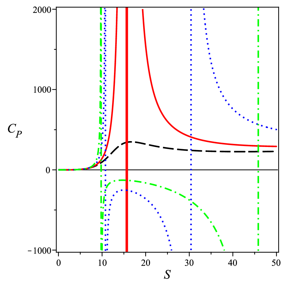
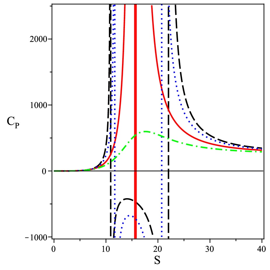
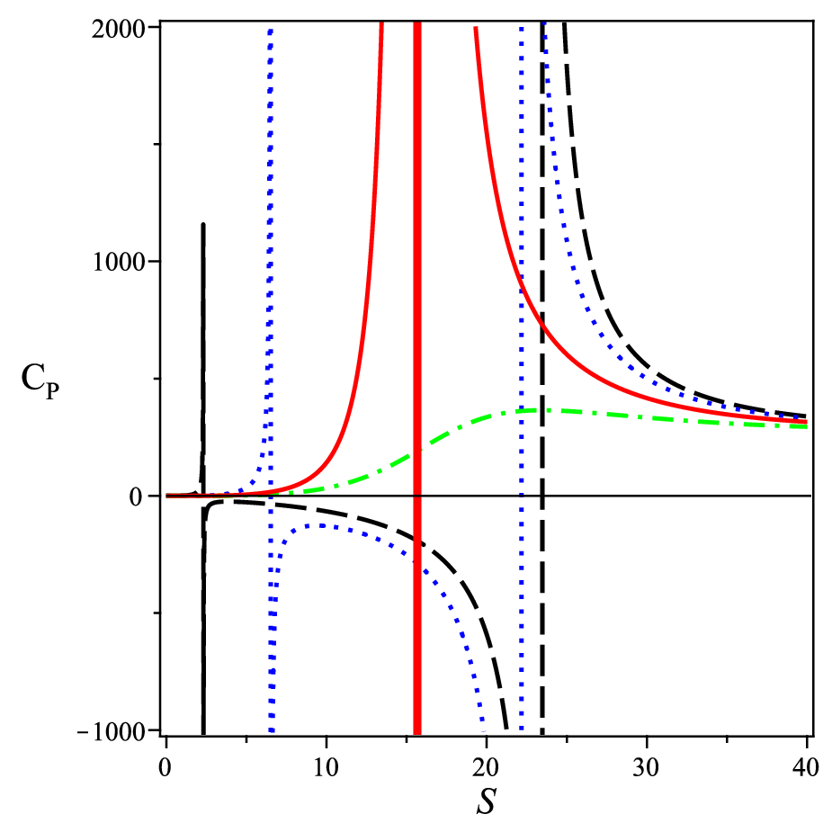
As can be seen from Fig. (8), there exist three different regions for . The partially positive specific heat for small black hole region and large black hole region means that those black holes are thermodynamically locally stable. Having negative specific heat of the intermediate black hole region represents a locally unstable system. The unstable region disappears at pressure resulting in a divergence point. When , is always positive and no divergent point exists. This means that in this case the black hole is local stable for arbitrary values of . In Fig. (8) and (8), the behavior of in terms of for different values of electric charge and angular momentum of black hole has been plotted. Obviously, at the critical pressure by increasing and the critical point disappears and black hole is stable.
The behavior of heat capacity could also represent the phase transitions. It
is clear that the heat capacity has at most two divergences which separate
small stable BHs, unstable region with medium horizon radius, and large
stable ones that are coincidence with extremum points of temperature and
Gibbs free energy. Also, the root of temperature coincides with the point
that the heat capacity changes its signature. The root separates the
non-physical solutions with negative temperature from physical black holes
with positive temperature (Fig. 9).
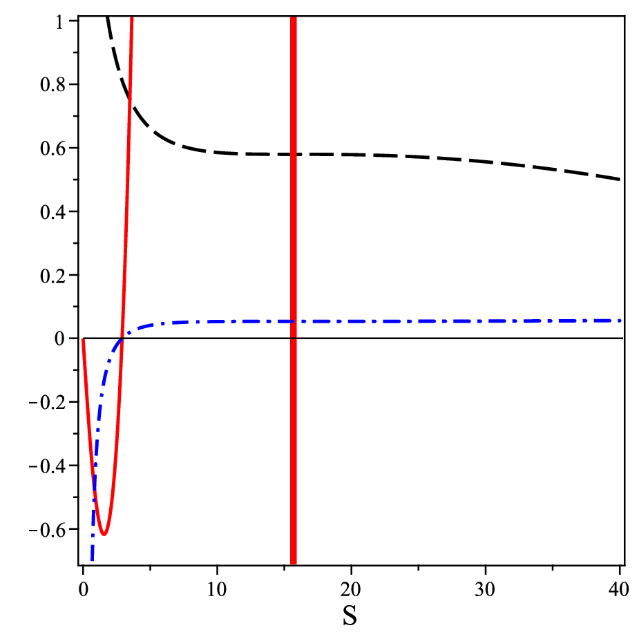

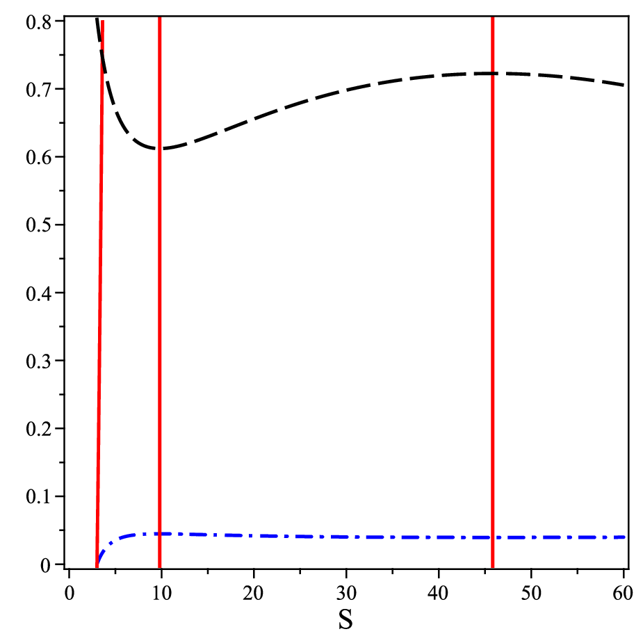
At the root the temperature is zero in which corresponds to the extremal configurations of black hole and leads to the maximum of the angular momentum such that
| (43) |
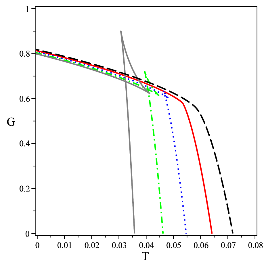
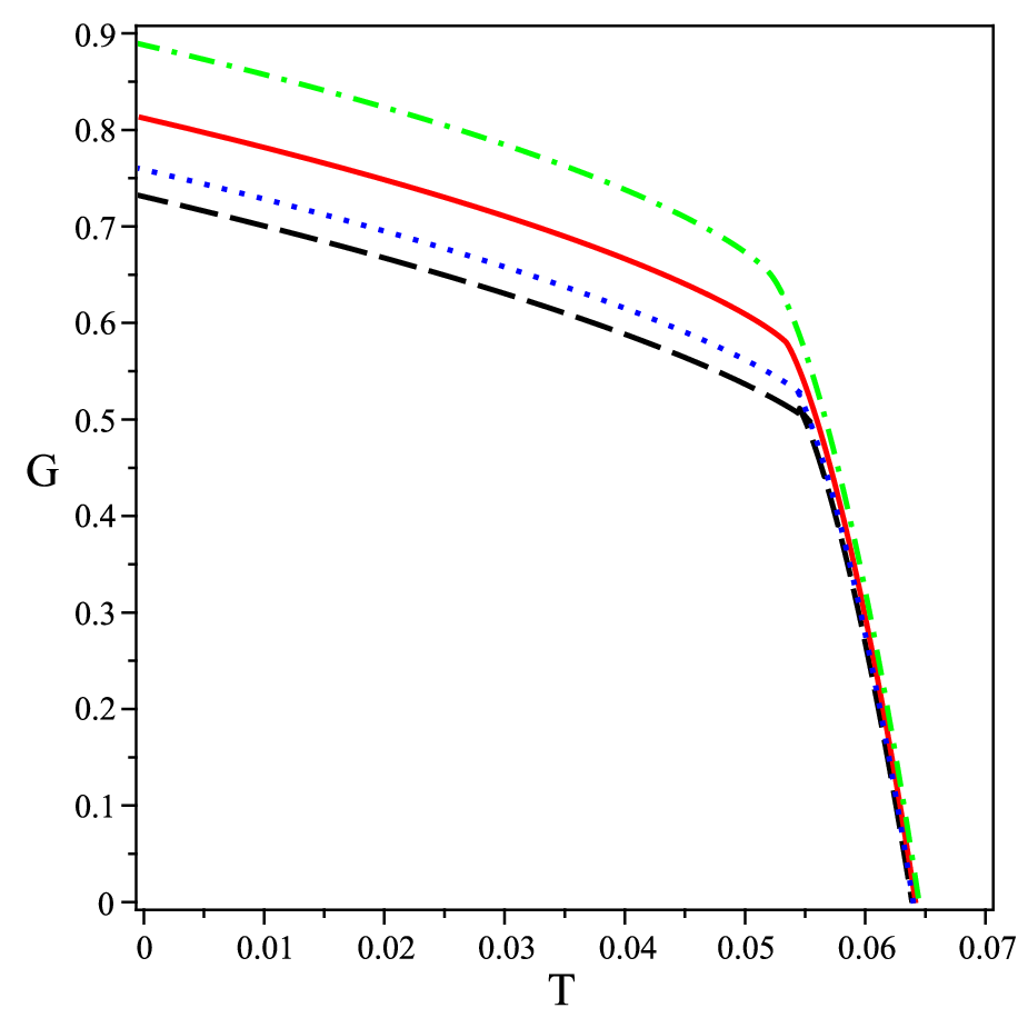
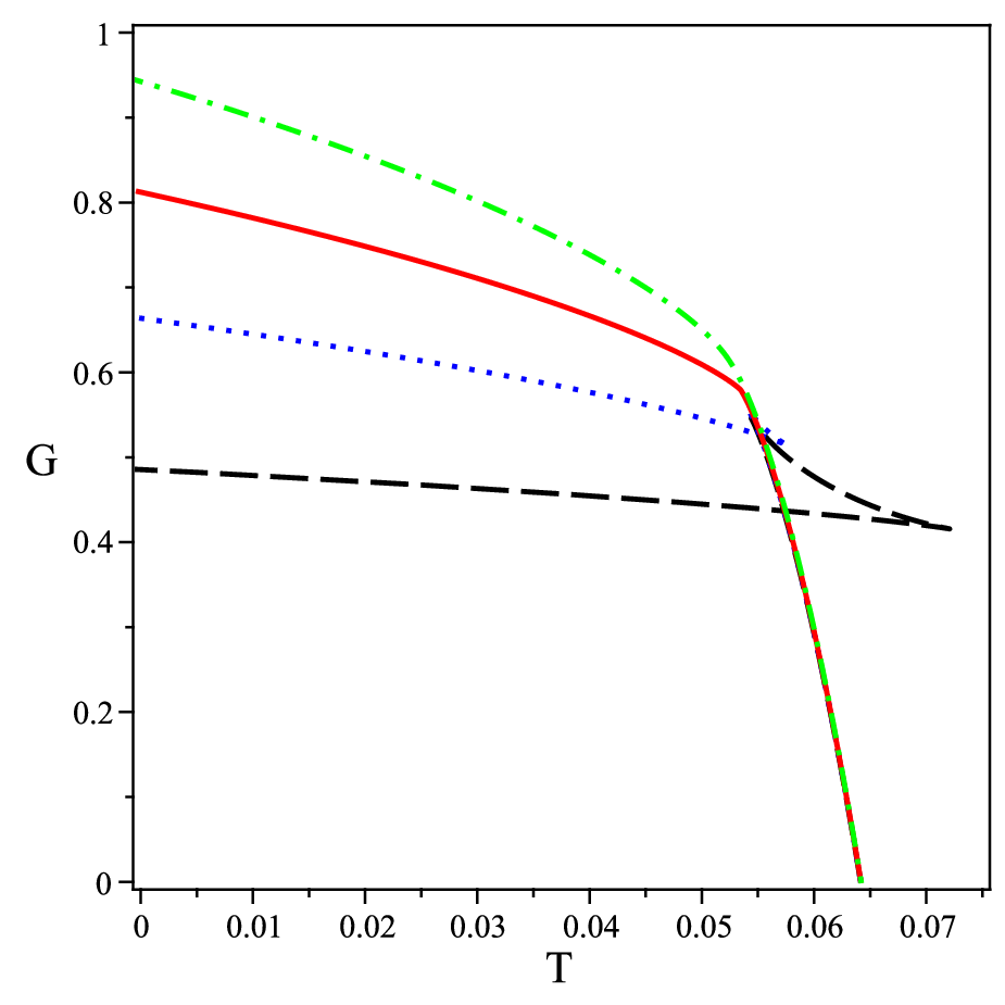
The plot of the Gibbs free energy with respect to the temperature shows a swallowtail behavior as presented in Fig. (10). When , the Gibbs free energy with respect to temperature develops a swallowtail like shape. There is a small/large first order phase transition in the black hole, which resembles the liquid/gas change of phase occurring in the van der Waals fluid. At the critical pressure , the swallowtail disappears which corresponds to the critical point. In the Fig. (10) and (10), we have represented the behavior of the Gibbs free energy in terms temperature for the different values of and . As can be seen, by increasing and the critical point disappears.
By using Eq. (32), we have plotted the pressure as a function of the event horizon radius in Fig. (11), keeping , and fixed. The temperature of isotherm diagrams decreases from top to bottom. The upper black solid line corresponds to the ideal gas phase, the critical isotherm is denoted by the red solid line, lower blue solid line corresponds to temperature smaller than the critical temperature and below the temperature the pressure becomes negative. Again, this is similar to the pressure-volume plot in van der Waals liquid/gas system.
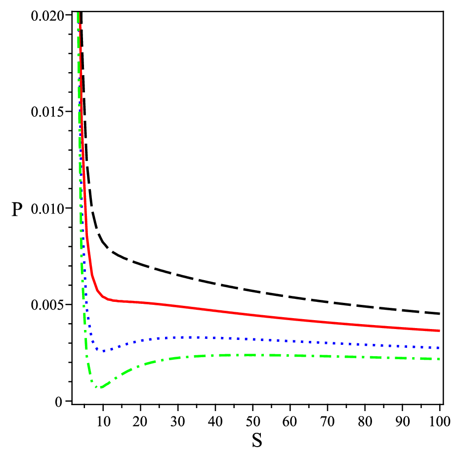
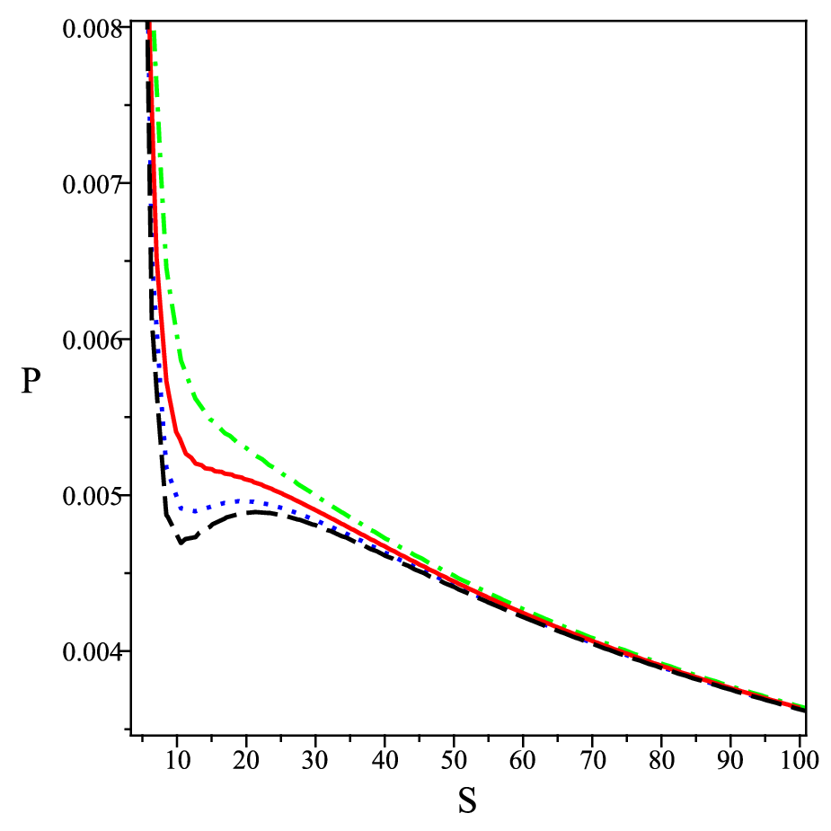
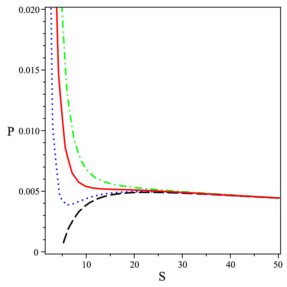
The isotherm corresponding to , has an inflection point. The corresponding pressure and entropy at that point are called critical pressure and critical entropy, respectively. So, the critical point is determined by
| (44) |
Using numerical methods for , we have and . Plugging these values into Eq. (22), one finds . By using of above consequence, one can achieve an approximately charge-independent result for the near universal ratio .
IV QNMs
It is possible to obtain an analytic relation for the real and imaginary parts of QNM as functions of the black hole charges () and of the gravitational perturbation field (). To do that, we obtain the field equation for the mass less scalar probe as follows
| (45) |
By using of two Killing vectors of the metric and , one can use the separation of variables of the scalar field as
| (46) |
Inserting Eq. (46) into (45) leads to two differential equations for the angular and radial terms of wave functions
| (47) |
| (48) |
where is a separation constant which can be obtained by using the boundary conditions of regularity at and . Since is a function of , we can calculate it, perturbatively, for small Casals:2018eev
| (49) |
where in the case of , we can write Casals:2018eev. In order to study QNMs, first one can change the radial coordinate to tortoise coordinate as follows
| (50) |
Now, we can find that black hole perturbations from equation (47) can be reduced to the following second-order ODE
| (51) |
where
| (52) |
So, for the slowly rotating and small charged black hole , and for the case and , the effective potential becomes
| (53) |
By using of Mashhoon’s method vf; Mashhoon:1985cya for QNMs, we can obtain an approximate expression for quasinormal frequencies.
At first, we should note that the maximum of occurs at
| (54) |
and therefore, is the radius of the photon sphere. The value of the maximum potential is
| (55) |
and the curvature parameter is given by vf; Mashhoon:1985cya
| (56) |
It should be noted that has a crucial role for all the above results. In order to obtain , we have inserted the above results in the equation (26) of Ref. Mashhoon:1985cya. Solving such a relation for , one can find the proper quasinormal frequencies as follows
| (57) |
where the real and imaginary parts of are, respectively,
| (58) |
and
| (59) |
It is noticable that all of the above results have been obtained in the case of .
As we know, in the eikonal limit there is a relation between the quasinormal frequencies and the properties of photon orbits. The real part of the quasinormal frequencies is related to the angular velocity of the photon orbit while the imaginary part is related to the Lyapunov exponent. In what follows, we want to investigate the relation between the real part of quasinormal modes and the radius of the shadow cast by the photon sphere of the black hole. To do so, we use the Hamilton-Jacobi Method to obtain the following equations of motion for null geodesics of charged rotating regular black hole at equatorial plane (see Appendix A) takahashi; mnv
| (60) |
where
| (61) |
| (62) | |||||
| (63) |
and
| (64) |
are two impact parameters. The conditions for the unstable circular orbits is given by . Now, one can easily obtain the expressions for and from the conditions of unstable circular orbits. For the generic , these parameters take the following simple forms
| (65) |
| (66) |
where is the radius of the unstable circular orbits. These two equations determine the contour of the shadow in plane. Furthermore, the radius of the shadow is calculated as
| (67) |
in which for the limit of and , we have
| (68) |
By inserting into the Eq. (54), one can obtain the radius of photon sphere as follows
| (69) |
It is obvious that in the limit and by inserting Eq. (69) for (at ) into the Eq. (68), we achieve
| (70) |
and it is easy to show that the real part of QNMs is inversely proportional to the shadow radius as follows
| (71) |
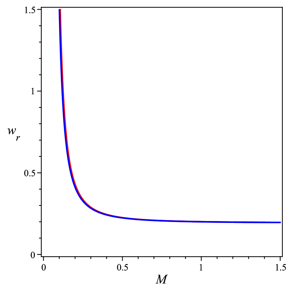
In the following, we want to obtain the connection between Lyapunov exponent and the imagenary parts of quasinormal mode (Eq. (59)). The Lyapunov behavior exists in the systems that sensitive to the initial conditions. So, the Lyapunov exponent which determines the value of the sensitvity should have behavior looks like the imagenary parts of quasinormal mode which determines instability of black hole. To extract the Lyapunov exponent, we follow the method of Ref. Mashhoon:1985cya. We perturb the equatorial geodesic equations (60) as
| (72) |
Here, by perturbing the radial equation to leading order in , we obtain
| (73) |
Now, by solving Eq. (73) and using the condition , we can find
| (74) |
So, by using of first equation for the radial and third equation for of Eqs. (60) and (65) and also the equation (54) for photon sphere radius in the limit of and , we can write
| (75) |
For the sake of completeness, we have done a comparison between Lyapunov exponent and imaginary part of quasinormal frequency in Fig. 13, and obviously, there is a good agreement between them.
V Conclusion
In this study, we have addressed a rotating regular black hole in the framework of Einstein’s general relativity coupled to a nonlinear electrodynamics. We have shown that for some values of parameters, there is an event horizon for nonsingular solution and we can interpret it as a black hole. In fact, we have obtained an upper limit for the magnetic charge or rotation parameter in order to have event horizon and ergosphere. We have plotted the ergoregion and have shown that as the magnetic charge and rotation parameter increased, the ergoregion also increased. Since thermodynamical behavior is of great importance in the search for a quantum theory of gravitation, we have also managed to perform a thermodynamic investigation of the black hole solutions. The conserved and thermodynamic quantities have been calculated and the validity of the first law has been examined. In addition, we have investigated the global stability of the black hole by plotting the Gibbs free energy. Also, the heat capacity has been studied to check the local stability. We have shown that the present solutions admitted small/large phase transitions similar to the van der Waals liquid/gas phase transition. Then, we have analytically studied the quasinormal modes of black hole by using of Mashhoon’s method. Finally, in order to obtain a relation between the quasinormal frequencies and the properties of the photon sphere, we have obtained the shadow radius of black hole and Lyapunov exponent. As it can be seen, there is a good agreement between the inverse of shadow radius and Lyapunov exponent with real and imaginary parts of quasinormal modes, respectively.
Acknowledgements
S. N. Sajadi acknowledge the support of Shiraz University.
Appendix A Effective potential
Here, we want to show why we have used the original metric instead of effective metric to study the shadow of black hole. As we know, photons in the nonlinear electrodynamics do follow the null geodesics of an effective metric rather than of the original one mnv. So, we need to study the effective metric. The effective geometry has been written as follows
| (76) |
So, the effective metric in the plane , can be written as
| (77) |
where
| (78) |
| (79) |
| (80) |
| (81) |
Here is the same as that of Eq. (16) but at and at . It is useful to study the effective potential that is felt by the photons. By using of the symmetries of the metric one can achieve to the following equation
| (82) |
where
| (83) |
and are the components of the metric, is the Killing vector and is the total energy. Considering Fig. 14, we give plots of for the metric (77)(blue line) and for metric (4)(red line). One can see that the difference between the two plots is insignificant and it is thus legitimate to use the original metric instead of effective one.

References
- (1) J. Bardeen, in Conference Proceedings of GR5 (USSR, Tbilisi, 1968), p. 174.
- (2) E. Ayon-Beato and A. Garcia, Phys. Rev. Lett. 80, 5056 (1998).
- (3) E. Ayon-Beato and A. Garcia, Phys. Lett. B 464, 25 (1999).
- (4) E. Ayon-Beato and A. Garcia, Gen. Rel. Grav. 31, 629 (1999).
- (5) E. Ayon-Beato and A. Garcia, Phys. Lett. B 493, 149 (2000).
- (6) L. Balart and E. C. Vagenas, Phys. Rev. D 90, 124045 (2014).
- (7) S. G. Ghosh, Eur. Phys. J. C 75, 532 (2015).
- (8) S. N. Sajadi and N. Riazi, Gen. Rel. Grav. 49, 45 (2017).
- (9) K. A. Bronnikov, Phys. Rev. D 64, 064013 (2001).
- (10) K. A. Bronnikov, Particles 1, 56 (2018).
- (11) K. A. Bronnikov, Phys. Rev. D 96, 128501 (2017).
- (12) K. Bronnikov, Phys. Rev. Lett. 85, 4641 (2000).
- (13) K. Bronnikov and J. Fabris, Phys. Rev. Lett. 96, 251101 (2006).
- (14) S. A. Hayward, Phys. Rev. Lett. 96, 031103 (2006).
- (15) W. Berej, J. Matyjasek, D. Tryniecki and M. Woronowicz, Gen. Rel. Grav. 38, 885 (2006).
- (16) I. Dymnikova, Class. Quant. Grav. 21, 4417(2004).
- (17) I. Dymnikova and E. Galaktionov, Class. Quant. Grav. 22, 2331(2005).
- (18) I. Dymnikova, Int. J. Mod. Phys. D 12, 1015(2003).
- (19) I. Dymnikova, Gen. Rel. Grav. 24, 235(1992).
- (20) B. P. Abbott and et al. [LIGO Scientific and Virgo Collaborations], Phys. Rev. Lett. 116, 061102 (2016).
- (21) B. P. Abbott and et al., [LIGO Scientific and Virgo Collaborations], Phys. Rev. Lett. 116, 241103 (2016).
- (22) B. P. Abbott and et al., [LIGO Scientific and Virgo Collaborations], Phys. Rev. Lett. 118, 241103 (2017).
- (23) K. Akiyama et al. [Event Horizon Telescope], Astrophys. J. 875, L1 (2019).
- (24) K. Akiyama et al. [Event Horizon Telescope], Astrophys. J. Lett. 875, L5 (2019).
- (25) K. Akiyama et al. [Event Horizon Telescope], Astrophys. J. Lett. 875, L6 (2019).
- (26) K. Akiyama et al. [Event Horizon Telescope], Astrophys. J. Lett. 875, L4 (2019).
- (27) E. T. Newman and A. I. Janis, J. Math. Phys. 6, 915 (1965).
- (28) I. Dymnikova and E. Galaktionov, Class. Quant. Grav. 32, 165015 (2015).
- (29) S. P. Drake and P. Szekeres, Gen. Rel. Grav. 32, 445 (2000).
- (30) C. Bambi and L. Modesto, Phys. Lett. B 721, 329 (2013).
- (31) S. P. Drake and R. Turolla, Class. Quant. Grav. 14, 1883 (1997).
- (32) D. J. C. Lombardo, Classical Quantum Gravity, 21, 1407 (2004).
- (33) R. Ferraro, Gen. Rel. Grav. 46, 1705 (2014).
- (34) M. Novello, V. A. De Lorenci, J. M. Salim and R. Klippert, Phys. Rev. D 61, 045001 (2000).
- (35) L. Modesto and P. Nicolini, Phys. Rev. D 82, 104035 (2010).
- (36) Y. Liao, X. B. Gong and J. S. Wu, Astrophys. J. 835, 247 (2017).
- (37) K. Jafarzade and J. Sadeghi, [arXiv:1710.08642].
- (38) R. T. Ndongmo, S. Mahamat, T. B. Bouetou and T. C. Kofane, [arXiv:1911.12521].
- (39) S. Haroon, M. Jamil, K. Jusufi, K. Lin and R. B. Mann, Phys. Rev. D 99, 044015 (2019).
- (40) M. Rizwan, M. Jamil and K. Jusufi, Phys. Rev. D 99, 024050 (2019).
- (41) H. Nollert, Phys. Rev. D 47, 5253 (1993).
- (42) S. Hod, Phys. Rev. Lett. 81, 4293 (1998).
- (43) G. T. Horowitz and V. E. Hubeny, Phys. Rev. D 62, 024027 (2000).
- (44) V. Cardoso and J. P. S. Lemos, Phys. Rev. D 64, 084017 (2001).
- (45) K. D. Kokkotas and B. G. Schmidt, Living Rev. Rel. 2, 2 (1999).
- (46) E. Berti, V. Cardoso and A. O. Starinets, Class. Quant. Grav. 26, 163001 (2009).
- (47) R. A. Konoplya and A. Zhidenko, Rev. Mod. Phys. 83, 793 (2011).
- (48) D. Kastor, S. Ray and J. Traschen, Class. Quant. Grav. 27, 235014 (2010).
- (49) F. Simovic and R. B. Mann, JHEP 1905, 136 (2019).
- (50) F. Simovic and R. B. Mann, Class. Quant. Grav. 36, 014002 (2019).
- (51) L. Balart and S. Fernando, Mod. Phys. Lett. A 32, 1750219 (2017).
- (52) L. Balart and E. C. Vagenas, Phys. Lett. B 730, 14 (2014).
- (53) L. Gulin and I. Smolic, Class. Quant. Grav. 35, 025015 (2018).
- (54) D. A. Rasheed, hep-th/9702087.
- (55) N. Breton, Gen. Rel. Grav. 37, 643 (2005).
- (56) B. P. Dolan, Class. Quant. Grav. 28, 125020 (2011).
- (57) B. P. Dolan, Class. Quant. Grav. 28, 235017 (2011).
- (58) M. Cvetic, G. W. Gibbons, D. Kubiznak and C. N. Pope, Phys. Rev. D 84, 024037 (2011).
- (59) D. Kubiznak and R. B. Mann, JHEP 1207, 033 (2012).
- (60) S. Gunasekaran, R. B. Mann and D. Kubiznak, JHEP 1211, 110 (2012).
- (61) A. Belhaj, M. Chabab, H. El Moumni and M. B. Sedra, Chin. Phys. Lett. 29, 100401 (2012).
- (62) R. Banerjee and D. Roychowdhury, Phys. Rev. D 85, 104043 (2012).
- (63) S. H. Hendi and M. H. Vahidinia, Phys. Rev. D 88, 084045 (2013).
- (64) N. Altamirano, D. Kubiznak, R. B. Mann and Z. Sherkatghanad, Class. Quant. Grav. 31, 042001 (2014).
- (65) N. Altamirano, D. Kubiznak, R. B. Mann and Z. Sherkatghanad, Galaxies 2, 89 (2014).
- (66) D. Kubiznak and R. B. Mann, Can. J. Phys. 93, 999 (2015).
- (67) C. V. Vishveshwara, Phys. Rev. D 1, 2870 (1970).
- (68) S. Chandrasekhar, Clarendon Press, Oxford, 1983.
- (69) F. J. Zerilli, Phys. Rev. Lett. 24, 737 (1970).
- (70) V. Ferrari and B. Mashhoon, Phys. Rev. D 30, 295 (1984).
- (71) B. Mashhoon, Phys. Rev. D 31, 290 (1985).
- (72) Y. Dcanini, A. Folacci, B. Raffaelli, Phys. Rev. D 81,104039 (2010) .
- (73) S. Fernando, J. Correa, Phys. Rev. D 86, 64039(2012).
- (74) A. Flachi, J. Lemos, Phys. Rev. D 87, 024034 (2013).
- (75) S. C. Ulhoa, Braz. Jour. Phys. 44, 380 (2014).
- (76) R. A. Konoplya and A. Zhidenko, JHEP 1709, 139 (2017).
- (77) S. N. Sajadi, N. Riazi and S. H. Hendi, Eur. Phys. J. C 79, 775 (2019).
- (78) S. Hod, Phys. Rev. Lett. 81, 4293 (1998).
- (79) S. Musiri and G. Siopsis, Phys. Lett. B 579, 25 (2004).
- (80) E. Abdalla, K. H. C. Castello-Branco and A. Lima-Santos, Mod. Phys. Lett. A 18, 1435 (2003).
- (81) E. Berti, V. Cardoso, K. D. Kokkotas and H. Onozawa, Phys. Rev. D 68, 124018 (2003).
- (82) V. Cardoso, A. S. Miranda, E. Berti, H. Witek and V. T. Zanchin, Phys. Rev. D 79, 064016 (2009).
- (83) I. Z. Stefanov, S. S. Yazadjiev and G. G. Gyulchev, Phys. Rev. Lett. 104, 251103 (2010).
- (84) K. Jusufi, arXiv:1912.13320 [gr-qc].
- (85) K. Jusufi, arXiv:2004.04664 [gr-qc].
- (86) Z. Y. Fan and X. Wang, Phys. Rev. D 94, 124027 (2016).
- (87) M. Casals and P. Zimmerman, Phys. Rev. D 100, 124027 (2019).
- (88) R. Takahashi, Publ. Astron. Soc. Jap. 57, 273 (2005).
- (89) E. Altas and B. Tekin, Phys. Rev. D 99, 044026 (2019).
- (90) M. M. Caldarelli, G. Cognola and D. Klemm, Class. Quant. Grav. 17, 399 (2000).