Causal representation of multi-loop Feynman integrands within the loop-tree dualityPreprint: IFIC/20-27
Abstract
The numerical evaluation of multi-loop scattering amplitudes in the Feynman representation usually requires to deal with both physical (causal) and unphysical (non-causal) singularities. The loop-tree duality (LTD) offers a powerful framework to easily characterise and distinguish these two types of singularities, and then simplify analytically the underling expressions. In this paper, we work explicitly on the dual representation of multi-loop Feynman integrals generated from three parent topologies, which we refer to as Maximal, Next-to-Maximal and Next-to-Next-to-Maximal loop topologies. In particular, we aim at expressing these dual contributions, independently of the number of loops and internal configurations, in terms of causal propagators only. Thus, providing very compact and causal integrand representations to all orders. In order to do so, we reconstruct their analytic expressions from numerical evaluation over finite fields. This procedure implicitly cancels out all unphysical singularities. We also interpret the result in terms of entangled causal thresholds. In view of the simple structure of the dual expressions, we integrate them numerically up to four loops in integer space-time dimensions, taking advantage of their smooth behaviour at integrand level.
1 Introduction
There is an important interest in considering higher order predictions in perturbation theory. This is due to the exceptional experimental measurements that have been done at the CERN’s Large Hadron Collider (LHC) Mangano:2020icy and, also, in view of future colliders Abada:2019lih; Abada:2019zxq; Benedikt:2018csr; Abada:2019ono; Blondel:2019vdq; Bambade:2019fyw; Roloff:2018dqu; CEPCStudyGroup:2018ghi. In general, multi-loop integrals are not always well defined in space-time dimensions. Hence, a special treatment needs to be carried out through dimensional regularisation (DREG) Bollini:1972ui; tHooft:1972tcz that introduces extra difficulties. Several alternative techniques have appeared in the recent years Gnendiger:2017pys that are aimed at overcoming this problem by keeping most of the computations in space-time dimensions.
Scattering amplitudes and loop integrals in the Feynman representation exhibit, in general, unphysical or non-causal singularities in the loop momentum space. Their representation in terms of Feynman parameters, Symanzik polynomials or Mellin-Barnes also inherit the unphysical structure of the original loop integral. However, all these unphysical singularities are expected to cancel after integration.
It would be therefore desirable to work with loop representations, in which the integrand would exclusively exhibit the physical or causal singularities that characterise the final integrated expression. On the one hand, such representations would be more stable and faster to integrate through numerical methods. On the other hand, the presence of non-causal singularities obscures and makes difficult the analysis of the actual singular structure through, e.g., the Landau equations Landau:1959fi, particularly at higher quantum orders.
One of the most appealing features of the loop-tree duality (LTD) Catani:2008xa; Bierenbaum:2010cy; Bierenbaum:2012th is that the unphysical or non-causal singularities cancel among different contributions of the integrand dual representation. This behaviour was firstly demonstrated for one-loop amplitudes Buchta:2014dfa; Buchta:2015wna and then to higher quantum orders Aguilera-Verdugo:2019kbz, and is the fundamental property that enables the simultaneous generation of loop and real-emission events through the four-dimensional unsubtraction (FDU) Hernandez-Pinto:2015ysa; Sborlini:2016gbr; Sborlini:2016hat. Other methods have also been proposed that are aimed at performing perturbative computations directly in the four physical space-time dimensions Fazio:2014xea; Bobadilla:2016scr; BaetaScarpelli:2001ix; BaetaScarpelli:2000zs; Pittau:2012zd; Page:2018ljf; Gnendiger:2017rfh; Bruque:2018bmy; Pozzorini:2020hkx.
The LTD formalism has recently taken also a lot of attention from other authors Tomboulis:2017rvd; Runkel:2019yrs; Runkel:2019zbm; Capatti:2019ypt. This is indeed due to the advantages of LTD in the numerical integration of loop integrals Buchta:2015xda; Buchta:2015wna; Capatti:2019edf and, therefore, scattering amplitudes Driencourt-Mangin:2017gop; Jurado:2017xut; Driencourt-Mangin:2019aix; Driencourt-Mangin:2019sfl; Driencourt-Mangin:2019yhu. In particular, an -point amplitude at loops requires, within the LTD approach, only integrations. Typically, this corresponds to the Euclidean space of the loop three-momenta, although LTD works as well in arbitrary coordinate systems. Since, in an Euclidean space, the hierarchies of scales are unambiguous, LTD has also been exploited as an alternative method Driencourt-Mangin:2017gop; Plenter:2019jyj; Plenter:2020lop for asymptotic expansions Beneke:1997zp. Moreover, extra external momenta and, likewise, internal propagators do not alter the number of integrations. Thus, the CPU time necessary for numerical integrations does not increase drastically with the number of external momenta as in other numerical approaches.
In a recent Letter Verdugo:2020kzh, we have conjectured that, in fact, LTD leads to loop integrand representations which are manifestly free of non-causal singularities to all orders and independently of the internal configuration. In this paper, we elaborate further on the conjecture of Ref. Verdugo:2020kzh, which claims that non-causal singularities can be eliminated at integrand level from its analytic expression, then, leading to unintegrated representations displaying causal singularities exclusively. In order to achieve this conclusion, we rely on the classification of parent topologies at multi-loop level defined in Ref. Verdugo:2020kzh, which are used as the building block to describe more complex topologies. In particular, two-loop scattering amplitudes can be characterised by a topology with momentum sets, where in each set there is an explicit dependence on the same loop momentum or a linear combination of the two loop momenta. The generalisation of this topology at multi-loop level, with momentum sets, is called Maximal Loop Topology (MLT). Similarly, the extension to loop configurations with and sets, with arbitrary, originates the Next-to-Maximal Loop Topology (NMLT) and the Next-to-Next-to-Maximal Loop Topology (N2MLT), respectively. Several relations exist among them through convolutions and factorisation identities, as presented in Ref. Verdugo:2020kzh. These are the only topologies necessary to describe any scattering amplitude of up to three loops. Beyond three loops, new topologies appear that are considered in another paper Ramirez-Uribe:2020hes.
Following this spirit, we present closed formulae for all the MLT, NMLT and N2MLT multi-loop topologies in terms of causal propagators only. We start from their compact LTD representations presented in Ref. Verdugo:2020kzh that contain both causal and non-causal singularities. Then, we reconstruct the full analytical result from numerical evaluations over finite fields vonManteuffel:2014ixa; Peraro:2016wsq. This reconstruction algorithm allows us to overcome the non-causal propagators, since cancellations of the latter are implicitly performed. To the best of our knowledge, the application of finite fields to generate integrands free of unphysical singularities is not present in the literature and is studied here for the first time. On top of it, the algorithm presented in this paper can be straightforwardly extended to any topology, NkMLT with , and arbitrary internal configurations.
For the purpose of elucidating the methods and results, we organise the paper in two parts. The first one corresponds to the explicit study of the three parent loop topologies, MLT, NMLT and N2MLT, first with single and then with multiple power propagators. We emphasise on the physical causal structure that the integrands display as a byproduct of the LTD representation. Traditional approaches based on integration-by-parts identities Chetyrkin:1981qh; Laporta:2001dd produce, in general, scalar integrals with powered propagators. The LTD approach allows, without modifying our algorithm, to consider as well all these configurations, and therefore provides the interplay between our approach and the traditional methods.
The second part concerns to the study of the numerical performance of the causal LTD representation of the MLT, NMLT and N2MLT topologies. We highlight that the structure of these compact formulae at loops allows us to have a smooth and well-behaved numerical evaluation. Certainly, with the presence of only physical singularities, we can elaborate more efficiently on the cancellation of the latter, following the lines of FDU Hernandez-Pinto:2015ysa; Sborlini:2016gbr; Sborlini:2016hat, in which the cancellation of infrared and ultraviolet singularities are performed at integrand level.
The paper is structured as follows. In Sec. 2, we recall the main features
of the all-order LTD representation with Lorentz-invariant infinitesimal
complex prescription of dual propagators Catani:2008xa; Bierenbaum:2010cy; Verdugo:2020kzh.
Then, in Sec. 3, on top of the general expressions for the MLT, NMLT and N2MLT
configurations given in Ref. Verdugo:2020kzh, we present their compact analogous expressions
in terms of exclusively causal propagators. In order to obtain this set of expressions,
we use analytic reconstruction over finite fields through the
C++ implementation, FiniteFlow Peraro:2019svx, of this algorithm
and interpret the results in terms of entangled causal thresholds.
In Sec. 4, elaborating on Sec 3, we study topologies
with higher powers in the propagators. We show that, independently of the powers
of the propagators, we end up with causal integrands.
These results are independent of the number of space-time dimensions.
Then, in Sec. 5, we numerically integrate the causal expressions obtained for
MLT, NMLT and N2MLT with linear and raised powers in the propagators.
In order to exploit the causal LTD representation,
we perform several numerical tests at space-time dimensions,
finding full agreement with softwares based on sector decomposition Hepp:1966eg; Roth:1996pd; Binoth:2000ps; Heinrich:2008si,
SecDec 3.0 Borowka:2015mxa and Fiesta 4.2 Smirnov:2015mct.
Finally, in Sec. 6, we draw our conclusions and future research directions.
Algebraic manipulations of this paper have been carried out with an in-house Mathematica implementation of the LTD theorem.
2 On the Loop-Tree Duality theorem to all orders
In this section, we set the notation and review the main features of the loop-tree duality (LTD) formalism. To start the discussion, let us consider a generic -point scattering amplitude at loops,
| (1) |
where, to simplify the notation, we use the shorthand notation for the integration measure, where corresponds to the independent loop momenta, is a function of the loop and external momenta , which is given by the Feynman rules of the theory. The function is defined as follows,
| (2) |
with the powers of the propagators and,
| (3) |
the usual Feynman propagator of one single particle, in which, corresponds to its mass, to the usual infinitesimal imaginary prescription and,
| (4) |
is the on-shell energy of the loop momentum written in terms of their spatial components . We have explicitly pulled out in Eq. (3) the dependence of the Feynman propagator on the energy component of the loop momentum because we will integrate out this component explicitly. In general, the LTD theorem is defined in arbitrary coordinate systems, as explained in Refs. Catani:2008xa; Bierenbaum:2010cy; Verdugo:2020kzh.
The sum inside the integrand of Eq. (1) accounts for all the Feynman diagrams, or sets of Feynman diagrams, that contribute to the scattering amplitude. In the context of integration-by-parts identities Chetyrkin:1981qh; Laporta:2001dd, Eq (1) can represent a single Feynman integral or a sum over master integrals.
Since all the propagators are written in terms of independent loop momenta, we classify them through the flowing between them. With this in mind, the set includes all the propagators with internal momenta of the form , where is a linear combination of external momenta and is the loop momentum, or the linear combination of loop momenta, that characterises the set. The number of different sets is always larger than the number of loops beyond one loop. For the sake of simplicity, we will consider from now on that each set is composed by only one propagator.
In order to obtain the LTD representation for a given scattering amplitude, it is necessary to apply the Cauchy residue theorem iteratively and integrate out one degree of freedom for each loop momentum. Then, in each iterative step, we select the poles with negative imaginary part in the complex plane of the component of the loop momentum that is integrated. In some intermediate steeps it is necessary to reverse some sets of momenta to keep a coherent momentum flow. A detailed discussion about this procedure is presented in Ref. Aguilera-Verdugo:2020nrp. Explicitly, starting from Eq. (1) and setting on shell the propagators that depend on the first loop momentum, , we define 11 1 For each loop, and w.r.t. Ref. Verdugo:2020kzh, the factor from the Cauchy residue theorem is now included in the integration measure, Eq. (7).,
| (5) |
where is the integrand of the amplitude in Eq. (1). The residue in Eq. (5) corresponds to integrate out the energy components of the loop momenta. Hence, assuming that the iteration goes until the -th set, we construct the nested residue as
| (6) |
The final LTD representation is given by the sum of all the nested residues and corresponds to setting simultaneously lines on shell, which is equivalent to open the loop amplitude to non-disjoint trees. In the following, we use the abbreviation
| (7) |
for the -momentum integration measure.
3 Causal representation of multi-loop integrals by analytic reconstruction
In former works Aguilera-Verdugo:2019kbz, we have demonstrated how the LTD formalism provides a comprehensive classification of causal singularities and how unphysical ones are cancelled among paired terms. These results stimulated the study of multi-loop topologies based on the definition of a systematic classification scheme, and leading to general LTD representations22 2 A formal inductive proof of the all-order validity of such representations is presented in Aguilera-Verdugo:2020nrp. of the MLT, NMLT and N2MLT topologies depicted in Fig. 1. In fact, along the same lines, these results have been extended to N4MLT Ramirez-Uribe:2020hes. In view of specific explicit examples, we also conjectured in Ref. Aguilera-Verdugo:2019kbz that LTD leads to integrand representations which are manifestly free of nonphysical singularities to all loop orders and regardless of the internal configuration. Hence, here and in the successive sections, we elaborate on this conjecture and present causal representations of MLT, NMLT and N2MLT to all loop orders.
Starting from the compact LTD representations of the NMLT and N2MLT multi-loop topologies
presented in Ref. Verdugo:2020kzh in terms of nested residues (6),
that contain both causal and non-causal singularities,
and motivated by their factorisation properties in terms of MLT subtopologies, for which we already obtained
a causal representation, namely, free of non-causal singularities,
we reconstruct in this section their full analytic expression in term of causal propagators only.
Here and in the following, we refer to causal propagators to denominators that only
contain sums of on-shell energies of the loop momenta,
,
whereas non-causal ones are expressed as denominators
that contain differences of
on-shell energies of the loop momenta,
,
leading thus to spurious singularities that are canceled as
shall be described in this section.
We perform this operation by numerical evaluation over finite fields vonManteuffel:2014ixa; Peraro:2016wsq,
in which we use the C++ implementation of the FiniteFlow Peraro:2019svx algorithm
together with its Mathematica interface.
In particular, we profit from the way how this algorithm solves linear systems.
Within the approach of reconstructing analytical expressions from numerical evaluations, we simply end up with rational functions, whose variables are the on-shell loop momenta and the energy components of the external momenta, . It turns out that this rational function is written only in terms of causal propagators Verdugo:2020kzh, which always have the structure of sums of on-shell loop energies. This pattern, indeed, shows a very interesting behaviour, since the numerical evaluation of these quantities lacks of possible zeroes due to the absence of differences of . As shall be described in the following, we comment more on this pattern, elucidating how our final formula, originally constructed from non-causal propagators, contains only causal ones, and we interpret the result in terms of entangled causal thresholds.
Furthermore, it is important to obtain a closed formula that can describe the pattern of any topology with an arbitrary number of loops. This, certainly, provides a parametric expression at all orders and, hence, the calculation through the nested residue (6) is avoided. In order to sketch our procedure to obtain the causal analytic expressions, we explicitly consider NMLT and N2MLT vacuum integrals first and then their generalisation with external momenta.
3.1 The two-loop sunrise diagram
Before starting with the analysis of the multi-loop MLT, NMLT and N2MLT configurations, let us consider, for illustrative reasons, the simplest example of the two-loop sunrise diagram with three propagators. Then, with the convention of (3), this two-loop integral becomes
| (8) |
with for , and . Thus, by applying the Cauchy residue theorem in , we obtain the LTD representation of in terms of the nested residues (6),
| (9) |
where the bar indicates a reversal of the momentum flow of the corresponding propagators, , and represents the double residue of the integrand of ,
| (10) |
Then, the first term of the integrand in Eq. (9),
| (11) |
allows us to implement the decomposition
| (12) |
where the first term on the r.h.s. of Eq. (12) represents the double residue over the positive energy mode of the propagator with momentum . This term generates a causal threshold at , if , when becomes on shell, and represents a configuration where the three on-shell momenta are aligned in the same direction. The second term in Eq. (12) is non-causal and shall cancel. Hence, by applying partial fractioning to the three contributions of (9), we notice that non-causal denominators are piecewise canceled, leading to,
| (13) |
which is manifestly free of non-causal thresholds. Besides the causal threshold which is active if , this expression also generates the complementary causal threshold for that arise when the three on-shell momenta flow in the opposite direction. In other words, when the three negative energy modes are selected and set on shell. If , both threshold configurations occur simultaneously, although only the limit , with , can lead to an integrand singularity.
We would like to remark that the ordering in which the residues are taken does not alter the final result given by Eq. (13), although individual terms are modified. For example, the expression
| (14) |
leads exactly to Eq. (13), although the individual contributions are different from those in Eq. (9) and also exhibits non-causal thresholds.
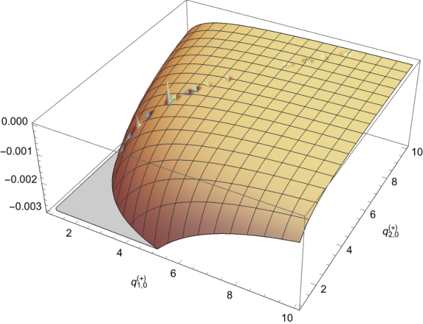
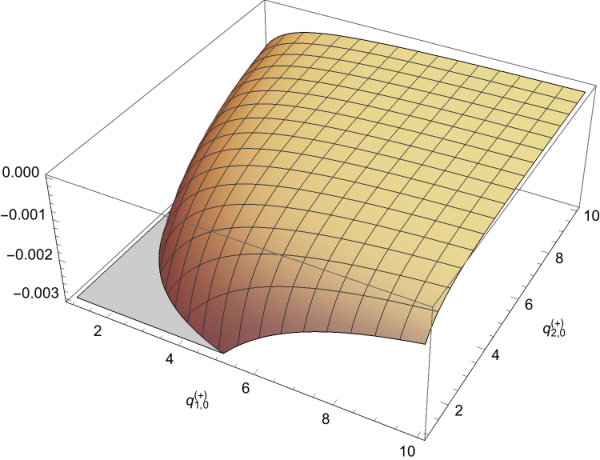
Let us now briefly comment on the structure of the two kind of integrands. Both representations, with or without non-causal thresholds, are physically equivalent. However, the LTD representation that still contains non-causal denominators is not optimal since it exhibits spurious singularities. This is illustrated in Fig. 2, where we show the difference between the full expression (9) and the simplified one (13). The small peaks in the left plot are due to numerical fluctuations introduced by the numerical cancellation of non-causal thresholds arising at (assuming ), which correspond to the singularities of the individual terms in (9).
3.2 Maximal Loop Topology
The MLT configuration is characterised by sets of propagators with an arbitrary number of propagators in each set. A pictorial representation of this topology is given in Fig. 1a. Its general LTD representation is given by Verdugo:2020kzh,
| (15) |
in terms of the nested residues defined in Eq. (9). This expression is valid for any loop integral or scattering amplitude with an arbitrary internal configuration, although it contains both causal and non-causal thresholds. Again, the bar in indicates a reversal of the momentum flow or equivalently a selection of negative energy modes.
For the sake of simplicity, we will consider in the following only one propagator in each set and scalar integrals. The momenta of these propagators are defined as follows.
| (16) |
The two-loop integral in Eq. (8) indeed belongs to the MLT family. Likewise, any two-loop amplitude can be cast in this way, independently on whether it contains planar or non-planar topologies. At this order, , there are only three independent sets of propagators.
A causal representation of this topology was already presented in Ref. Verdugo:2020kzh,
| (17) |
where means that the external momentum has been inserted in the loop momentum according to (16), and,
| (18) |
Due to the simplicity that this set of integrals holds, we have used it as a first test of the reconstruction algorithm that is explained later. By setting , we recover (13).
Each of the two terms of the integrand in Eq. (17) represents a potential causal threshold singularity. Only one of them is active once the sign of the energy of the external momentum, , is fixed. These two causal thresholds can be interpreted exactly as we interpreted Eq. (13). The threshold singularities arise when all the momenta are on shell and either aligned in one direction or the opposite one. The graphical interpretation of these causal thresholds is illustrated in Fig. 3.
3.3 NMLT vacuum integral
As we have observed, the MLT topology is sufficient to describe any two-loop configuration. Starting from three loops, the NMLT and N2MLT topologies are also necessary to characterise the loop configurations that are not described by MLT. General LTD representations for NMLT and N2MLT have been presented in Ref. Verdugo:2020kzh that contain both causal and non-causal thresholds. In this section, we consider their causal LTD representation. To simplify the presentation, we start by considering configurations with one single propagator in each set, and no external momenta. The more complex case with external momenta will be considered in Sec. 3.5. Then, to describe NMLT configurations, on top of considering the internal momenta (16), with , we also need to add an additional one,
| (19) |
A pictorial representation of NMLT is provided in Fig 1b.
The causal LTD representation that we obtain is
| (20) |
with
| (21) |
This expression, although it is slightly more complicated than the MLT one, can easily be rewritten by partial fractioning in the more suitable form,
| (22) |
The analytic expression of Eq. (22) can alternatively be reconstructed from numerical evaluations over finite fields. Since the integrand in (20) is a rational function in the on-shell energies of the loop momenta, , we find relations among and . For instance, at , we find
| (23) | ||||||
Then, by plugging these relations in (20), we directly find (22). Because the numerator of (20) is a linear function of , both approaches are of the same difficulty.
In this particular case, it is straightforward to observe the linear relations between and , leading, in this way, to simplifications originated by polynomial divisions. In fact, as stated above, Eq. (20) can be directly obtained by using partial fractioning. In more general cases, partial fractioning will produce more terms that need to be properly canceled. Hence, to avoid the proliferation of terms at intermediate steps, we make use of the analytic reconstruction over finite fields to obtain compact expressions containing only causal propagators. In the following section, we shall note that simplifications are not straightforward because the degree of the numerator we want to reduce increases as the number of causal propagators.
Let us now interpret (22) in terms of what we call entangled causal thresholds. Each of the represents a potential causal threshold singularity that, as in the MLT case, requires that all the momentum flows are aligned in the same direction. The product of two causal denominators can be understood as representing physical configurations where two sets of propagators can simultaneously go on shell. For this to happen, the common propagators have to be in the same configuration. This entanglement can also be understood from the factorisation identity that NMLT fulfils in terms of MLT subtopologies, as explained in Ref. Verdugo:2020kzh.
A pictorial interpretation of the entangled causal structure of (22) is provided in Fig. 4, where the dashed lines single out the internal propagators that eventually go on shell simultaneously; a subset of them is already on shell through LTD. Each diagram in Fig. 4 has two dashed lines that correspond to the two denominators and which are present in each term of (22). The causal thresholds are entangled because the momentum flow of the propagators that are common to both causal thresholds are matched. For example, the first diagram of Fig. 4 represents the term corresponding to the causal thresholds and that share the entangled propagators .
3.4 N2MLT vacuum integral
The N2MLT is the last topology that is needed to describe any full scattering amplitude at three loops. In fact, N2MLT is the master topology that describes also MLT and NMLT configurations to all orders Verdugo:2020kzh. This configuration is depicted in Fig. 1c, and is usually called Mercedes–Benz topology. Similar to the NMLT case, besides considering the internal momenta (16) and (19), we add one more,
| (24) |
For the moment, we consider configurations without external momenta. Then, with internal propagators, we have all the required ingredients to understand the structure of any integral at three loops and, equivalently, any scattering amplitude.
Hence, from the LTD representation of N2MLT given in Ref. Verdugo:2020kzh, we end up with the integrand written as a rational function,
| (25) |
with through defined in Eq. (21),
| (26) |
and a degree-four polynomial in . From the structure of the latter it is not straightforward to make manifest an expression with the features of Eqs. (17) and (22). Thus, we reconstruct its analytic expression through finite fields. In fact, one notices that the denominators are not independent; they, instead, obey a few relations. Hence, we write some and in terms of ,
| (27) | ||||||
Then, by properly replacing and , according to their relations and performing a straightforward polynomial division, we find,
| (28) |
Analogous to the NMLT case, we note that (28) is written to all orders in term of causal propagators only, in this case in terms of the product of three causal propagators. This pattern can be understood from two approaches. First, from their factorisation properties in terms of MLT and NMLT configurations, as explained in Ref. Verdugo:2020kzh. Second, from the entanglement of three causal thresholds. A pictorial representation of this entanglement is presented in Fig. 5 for the first term in the r.h.s. of (28).
3.5 NMLT and N2MLT topologies with external momenta
In this section, we show how to generalise the causal representations of the NMLT and N2MLT vacuum diagrams presented in Sections 3.3 and 3.4 to the most general case that considers insertion of external momenta. Then, to obtain analytic and compact expressions for these two topologies, we follow the same algorithm based on finite fields. The vacuum expression in Eqs. (22) and (28) have been used to guide this computation. Let us anticipate that the insertion of external momenta does not affect the causal physical behaviour of these integrals. The only difference now is that, as for the causal MLT representation given in Section 3.2, we have to distinguish the entangled configurations that correspond to external momenta with positive or negative energy flow, or in other words, if the external momenta are incoming or outgoing.
We can apply the same procedure for the insertion of the external momenta , and in the internal momenta , and , respectively,
| (29) |
The three external momenta are considered to have positive energy when they are incoming. By momentum conservation, we should also have either for NMLT or for N2MLT as outgoing momentum in one of the vertices. Besides, we emphasise that we set for NMLT while keeping the definition of the internal momenta at (29). These topologies, with the insertion of external momenta, are depicted in Fig. 6.
We note that the causal propagators are now shifted by the external momenta or a linear combination of them as
| (30) | ||||||
With the formula that we present in the following, we can describe, with a single representation, up to three-point functions for NMLT and up to four-point functions for N2MLT.
The causal representation of NMLT is a function of through , with , and is given by
| (31) |
Due to the insertion of external momenta, we have now to consider the entangled threshold configurations that distinguish if the external momenta are incoming or outgoing, namely, if their energy flow is positive or negative. With our conventions, positive energy flows correspond to incoming momenta. The exchange accounts for the configurations with opposite momentum flows and results in a doubling of the terms obtained for the vacuum diagrams.
The causal N2MLT representation also exhibits a very compact expression
| (32) |
Let us briefly summarise on the algorithm used to compute all these formulae.
As mentioned before, we profit from the software
FiniteFlow and its built-in functions, FFLinearFit and FFDenseSolve,
to analytically reconstruct the rational function of the configuration and
to find relations between and , respectively.
We would like to remark that these expressions for MLT, NMLT and N2MLT
have been analytically checked, with the iterated application of the LTD
theorem, up to six loops, finding completely agreement.
The pattern displayed by all topologies allows us to generalise
and provide a closed formula that has the mathematical support
of the studies carried out in Verdugo:2020kzh; Aguilera-Verdugo:2020nrp to all orders.
In other words, only causal contributions remain in the final expressions, being all
the non-causal or unphysical terms cancelled at intermediate steps.
We also note that the structure of the integrands suggests a smooth numerical
evaluation, which we profit in Sec. 5. Although we have presented explicit
expressions only for scalar integrals, the algorithm is valid as well for non-scalar integrals.
4 Topologies with higher powers in the propagators
So far we have discussed the structure of MLT, NMLT and N2MLT configurations in which the dependence on the Feynman propagators is linear. However, in practical applications, like UV local renormalisation Driencourt-Mangin:2017gop; Driencourt-Mangin:2019aix; Driencourt-Mangin:2019yhu or multi-loop calculations, one also deals with higher powers in the propagators Chetyrkin:1981qh; Laporta:2001dd; Bierenbaum:2012th. In this section, we elaborate on the compact formulae, found in the previous section, and provide a procedure for computing -loop integrals with higher powers in the propagators. In particular, due to the causal structure observed in all the cases, it is expected that this physical behaviour should also remain with higher powers of the propagators. Abusing of the notation and recalling we are considering only one propagator in each loop set, let us define,
| (33) |
with , for any -loop integral, where the superscript corresponds to the power of the -th propagator. In the following, for the sake of the simplicity, we restrict our study to the scalar case in which the numerator is .
Remarkably, due to the structure of the Feynman propagator (3), it is straightforward to raise the power in the propagators by simple performing derivatives w.r.t. ,
| (34) |
Therefore, the results obtained in Sec. 3 can be used for the purpose of the present discussion. Furthermore, we stress that the expressions obtained in the present paper are valid in any dimension, since only the energy components of the loop momenta have been integrated. Hence, we can yet numerically evaluate these integrals in any integer dimensions. Since the LTD representation of the Nk-1MLT configurations that we have considered are manifestly free of non-causal propagators, the corresponding loop integrals with raised propagators will also be causal. In the following we will consider integrals that are ultraviolet and infrared finite in order to check the better numerical performance of the causal LTD representation.
Therefore, if we were to evaluate finite integrals, for instance in integer space-time dimensions, it is sufficient to consider the causal LTD representation with linear propagators and perform the derivatives in the on-shell energies . For example, the MLT configuration, with the insertion of an external momentum,
| (35) |
In order to elucidate the operation of raising powers, we consider the simplest case with one single squared propagator. Since the denominators depend linearly on , we utilise the chain rule as follows,
| (36) |
This amounts to,
| (37) |
In the following, we present the numerical evaluation of several MLT, NMLT and N2MLT configurations. We remark that, within LTD, the inclusion of internal masses do not stem any issue. In more details, one needs to perform integrations for each loop. The number of integrations turn out to be lower than approaches based on Feynman parametrisation.
5 Numerical evaluation of Nk-1MLT
In view of the results of Secs. 3 and 4, we elaborate on those expressions by numerically integrating in the -loop momenta, . This is indeed done to investigate the stability of this set of formulae, written now in terms of causal propagators only. To this end, we evaluate multi-loop integrals in space-time dimensions 33 3 The case with space-time dimensions Runkel:2019zbm is trivial. One just replaces . , presenting results for topologies with and without higher powers in the propagators up to four loops.
The numerical results presented in this section are double checked with the softwares SecDec 3.0 and Fiesta 4.2.
5.1 Two-dimensional integrals
We start with the first non-trivial numerical application at space-time dimensions, in which we perform -loop integrations, one integration per loop. In order to perform these integrations, we embed the integration domain, , in a -dimensional sphere. This set of integration variables has the features that only one variable goes to infinity,
| (38) |
which we can compactify. Then, its domain is mapped onto through to the change of variable,
| (39) |
These operations are carried out in Mathematica as well as the numerical integration,
which was performed with the built-in function NIntegrate.
Then, with all the ingredients ready to perform the integrations, we evaluate the multi-loop integrals in which the propagators of the lines (16) have mass , while the remaining ones have mass . Likewise, to test the smooth behaviour of these integrations, we scan over . Here and in the following, all kinematic invariants are implicitly given in GeV2. We then integrate numerically up to four loops the MLT, NMLT and N2MLT topologies presented in Sec. 3. Nevertheless, the extension to higher loops does not originate any obstacle within our approach.
The evaluation of the two-dimensional integrals is shown in Fig. 7, where solid lines corresponds to the evaluation within LTD, and the dots represent the evaluations performed by Fiesta 4.2 and SecDec 3.0. The evaluation time per point was in a desktop machine with an Intel i7 (3.4GHz) processor with 8 cores and 16 GB of RAM. Additionally, we report that when including more propagators or, equivalently, inserting external momenta, the number of integrations for the softwares based on sector decomposition increases w.r.t. the number of Feynman parameters, instead, within LTD, one always has to perform integrations.
5.2 Three- and four-dimensional integrals
It is clear that the number of integrations depends on the dimensionality of the loop momenta. Hence, we can still use the same procedure of Sec. 5.1 to express all loop components in terms of spherical coordinates. Thanks to the LTD theorem, we pass from Minkowskian to Euclidean space, which, in practice, corresponds to work in . Hence, the embedding in a -dimensional sphere can be carried out analogously as in the former section.
Alternatively, an equivalent approach consists in treating each loop momentum independently when doing the change of variables. For instance, the integration domain can be separately expressed as follows,
| (40) |
where each term in the product is the -dimensional space of each loop momentum. The main difference between this approach and the former one relies on how the integrand behaves at infinity. In particular, embedding the integrand in a -dimensional sphere allows us to reach and understand this behaviour with a single variable. Instead, in the product of -dimensional spheres (40), this behaviour is understood with variables. In the present discussion, we, nonetheless, follow both approaches as a double check of our results.
6 Conclusions
In this paper, we have explicitly elaborated on the analytical structure of the Maximal (MLT), Next-to-Maximal (NMLT) and Next-to-Next-to-Maximal (N2MLT) loop topologies to all orders. We noted that any multi-loop scattering amplitude constructed from the MLT, NMLT and N2MLT topologies, within the loop-tree duality formalism, can always be expressed in terms of causal propagators only. The causal representation contains products of causal propagators that can be interpreted as entangled thresholds.
In order to understand the pattern of the multi-loop MLT, NMLT and N2MLT topologies, we reconstructed their compact analytic expressions and, thus, elucidated their causal structure. We made use of reconstruction of analytic expressions from numerical evaluations over finite fields, and generated compact formulae at arbitrary numbers of loops. The calculation of the compact causal formulae was explicitly carried out for multi-loop vacuum integrals as well as for their extension with external momenta.
We also studied the behaviour of topologies with higher powers in the propagators. In particular, we noted that the results generated for topologies with single power propagators give the relevant causal information. Hence, due to the explicit dependence in the on-shell loop energies of the LTD representation, we defined an operator that raises the powers of propagators starting from the original single-power causal representation.
In view of the compact and simple expressions of MLT, NMLT and N2MLT, we integrated them numerically up to four loops in integer space-time dimensions, . Since we had to perform integrations, we followed two approaches to evaluate these integrals. The first one embeds the integration domain in sphere, whereas the second one embeds the former in products of spheres. We found agreement in both approaches. Furthermore, we checked our expressions with available softwares based on sector decomposition, Fiesta 4.2 and SecDec 3.0.
The algorithm presented in this paper and the interpretation in terms of entangled causal thresholds can be extended to other loop integrals with more complex internal configurations and to new Nk-1MLT topologies, with , that will appear beyond three loops. We recall that a causal representation is expected, since in the end Nk-1MLT admits a decomposition in terms of MLT subtopologies.
Acknowledgements
This work is supported by the Spanish Government (Agencia Estatal de Investigación) and ERDF funds from European Commission (Grant No. FPA2017-84445-P), Generalitat Valenciana (Grant No. PROMETEO/2017/053) and the COST Action CA16201 PARTICLEFACE. R.J.H.-P. acknowledges support from Departament de Física Teòrica, Universitat de València, CONACyT through the Project No. A1-S-33202 (Ciencia Básica) and Sistema Nacional de Investigadores; W.J.T. from Juan de la Cierva program (FJCI-2017-32128), and J.J.A.V. from Generalitat Valenciana (GRISOLIAP/2018/101).
References
- (1) M. Mangano, LHC at 10: the physics legacy, 2003.05976.
- (2) FCC collaboration, A. Abada et al., FCC Physics Opportunities: Future Circular Collider Conceptual Design Report Volume 1, Eur. Phys. J. C 79 (2019) 474.
- (3) FCC collaboration, A. Abada et al., FCC-ee: The Lepton Collider: Future Circular Collider Conceptual Design Report Volume 2, Eur. Phys. J. ST 228 (2019) 261–623.
- (4) FCC collaboration, A. Abada et al., FCC-hh: The Hadron Collider: Future Circular Collider Conceptual Design Report Volume 3, Eur. Phys. J. ST 228 (2019) 755–1107.
- (5) FCC collaboration, A. Abada et al., HE-LHC: The High-Energy Large Hadron Collider: Future Circular Collider Conceptual Design Report Volume 4, Eur. Phys. J. ST 228 (2019) 1109–1382.
- (6) A. Blondel, J. Gluza, S. Jadach, P. Janot and T. Riemann, eds., Theory for the FCC-ee: Report on the 11th FCC-ee Workshop Theory and Experiments, vol. 3/2020 of CERN Yellow Reports: Monographs, (Geneva), CERN, 5, 2019. 10.23731/CYRM-2020-003.
- (7) P. Bambade et al., The International Linear Collider: A Global Project, 1903.01629.
- (8) CLIC, CLICdp collaboration, The Compact Linear e+e- Collider (CLIC): Physics Potential, 1812.07986.
- (9) CEPC Study Group collaboration, M. Dong et al., CEPC Conceptual Design Report: Volume 2 - Physics & Detector, 1811.10545.
- (10) C. G. Bollini and J. J. Giambiagi, Dimensional Renormalization: The Number of Dimensions as a Regularizing Parameter, Nuovo Cim. B12 (1972) 20–26.
- (11) G. ’t Hooft and M. J. G. Veltman, Regularization and Renormalization of Gauge Fields, Nucl. Phys. B44 (1972) 189–213.
- (12) C. Gnendiger et al., To , or not to : recent developments and comparisons of regularization schemes, Eur. Phys. J. C77 (2017) 471, [1705.01827].
- (13) L. Landau, On analytic properties of vertex parts in quantum field theory, Nucl. Phys. 13 (1960) 181–192.
- (14) S. Catani, T. Gleisberg, F. Krauss, G. Rodrigo and J.-C. Winter, From loops to trees by-passing Feynman’s theorem, JHEP 09 (2008) 065, [0804.3170].
- (15) I. Bierenbaum, S. Catani, P. Draggiotis and G. Rodrigo, A Tree-Loop Duality Relation at Two Loops and Beyond, JHEP 10 (2010) 073, [1007.0194].
- (16) I. Bierenbaum, S. Buchta, P. Draggiotis, I. Malamos and G. Rodrigo, Tree-Loop Duality Relation beyond simple poles, JHEP 03 (2013) 025, [1211.5048].
- (17) S. Buchta, G. Chachamis, P. Draggiotis, I. Malamos and G. Rodrigo, On the singular behaviour of scattering amplitudes in quantum field theory, JHEP 11 (2014) 014, [1405.7850].
- (18) S. Buchta, G. Chachamis, P. Draggiotis and G. Rodrigo, Numerical implementation of the loop–tree duality method, Eur. Phys. J. C77 (2017) 274, [1510.00187].
- (19) J. J. Aguilera-Verdugo, F. Driencourt-Mangin, J. Plenter, S. Ramírez-Uribe, G. Rodrigo, G. F. Sborlini et al., Causality, unitarity thresholds, anomalous thresholds and infrared singularities from the loop-tree duality at higher orders, JHEP 12 (2019) 163, [1904.08389].
- (20) R. J. Hernandez-Pinto, G. F. R. Sborlini and G. Rodrigo, Towards gauge theories in four dimensions, JHEP 02 (2016) 044, [1506.04617].
- (21) G. F. R. Sborlini, F. Driencourt-Mangin, R. Hernandez-Pinto and G. Rodrigo, Four-dimensional unsubtraction from the loop-tree duality, JHEP 08 (2016) 160, [1604.06699].
- (22) G. F. R. Sborlini, F. Driencourt-Mangin and G. Rodrigo, Four-dimensional unsubtraction with massive particles, JHEP 10 (2016) 162, [1608.01584].
- (23) R. A. Fazio, P. Mastrolia, E. Mirabella and W. J. Torres Bobadilla, On the Four-Dimensional Formulation of Dimensionally Regulated Amplitudes, Eur. Phys. J. C74 (2014) 3197, [1404.4783].
- (24) W. J. Torres Bobadilla, Generalised unitarity for dimensionally regulated amplitudes within FDF, PoS RADCOR2015 (2016) 063, [1601.05742].
- (25) A. Baeta Scarpelli, M. Sampaio, B. Hiller and M. Nemes, Chiral anomaly and CPT invariance in an implicit momentum space regularization framework, Phys. Rev. D 64 (2001) 046013, [hep-th/0102108].
- (26) A. Baeta Scarpelli, M. Sampaio and M. Nemes, Consistency relations for an implicit n-dimensional regularization scheme, Phys. Rev. D 63 (2001) 046004, [hep-th/0010285].
- (27) R. Pittau, A four-dimensional approach to quantum field theories, JHEP 1211 (2012) 151, [1208.5457].
- (28) B. Page and R. Pittau, NNLO final-state quark-pair corrections in four dimensions, Eur. Phys. J. C 79 (2019) 361, [1810.00234].
- (29) C. Gnendiger and A. Signer, in the four-dimensional helicity scheme, Phys. Rev. D 97 (2018) 096006, [1710.09231].
- (30) A. Bruque, A. Cherchiglia and M. Pérez-Victoria, Dimensional regularization vs methods in fixed dimension with and without , JHEP 08 (2018) 109, [1803.09764].
- (31) S. Pozzorini, H. Zhang and M. F. Zoller, Rational Terms of UV Origin at Two Loops, JHEP 05 (2020) 077, [2001.11388].
- (32) E. Tomboulis, Causality and Unitarity via the Tree-Loop Duality Relation, JHEP 05 (2017) 148, [1701.07052].
- (33) R. Runkel, Z. Szőr, J. P. Vesga and S. Weinzierl, Causality and loop-tree duality at higher loops, Phys. Rev. Lett. 122 (2019) 111603, [1902.02135].
- (34) R. Runkel, Z. Szőr, J. P. Vesga and S. Weinzierl, Integrands of loop amplitudes within loop-tree duality, Phys. Rev. D 101 (2020) 116014, [1906.02218].
- (35) Z. Capatti, V. Hirschi, D. Kermanschah and B. Ruijl, Loop-Tree Duality for Multiloop Numerical Integration, Phys. Rev. Lett. 123 (2019) 151602, [1906.06138].
- (36) S. Buchta, Theoretical foundations and applications of the Loop-Tree Duality in Quantum Field Theories. PhD thesis, Valencia U., 2015. 1509.07167.
- (37) Z. Capatti, V. Hirschi, D. Kermanschah, A. Pelloni and B. Ruijl, Numerical Loop-Tree Duality: contour deformation and subtraction, JHEP 04 (2020) 096, [1912.09291].
- (38) F. Driencourt-Mangin, G. Rodrigo and G. F. Sborlini, Universal dual amplitudes and asymptotic expansions for and in four dimensions, Eur. Phys. J. C 78 (2018) 231, [1702.07581].
- (39) J. L. Jurado, G. Rodrigo and W. J. Torres Bobadilla, From Jacobi off-shell currents to integral relations, JHEP 12 (2017) 122, [1710.11010].
- (40) F. Driencourt-Mangin, G. Rodrigo, G. F. R. Sborlini and W. J. Torres Bobadilla, Universal four-dimensional representation of at two loops through the Loop-Tree Duality, JHEP 02 (2019) 143, [1901.09853].
- (41) F. Driencourt-Mangin, Four-dimensional representation of scattering amplitudes and physical observables through the application of the Loop-Tree Duality theorem. PhD thesis, U. Valencia (main), 2019. 1907.12450.
- (42) F. Driencourt-Mangin, G. Rodrigo, G. F. Sborlini and W. J. Torres Bobadilla, On the interplay between the loop-tree duality and helicity amplitudes, 1911.11125.
- (43) J. Plenter, Asymptotic Expansions Through the Loop-Tree Duality, Acta Phys. Polon. B 50 (2019) 1983–1992.
- (44) J. Plenter and G. Rodrigo, Asymptotic expansions through the loop-tree duality, Eur. Phys. J. C 81 (2021) 320, [2005.02119].
- (45) M. Beneke and V. A. Smirnov, Asymptotic expansion of Feynman integrals near threshold, Nucl. Phys. B522 (1998) 321–344, [hep-ph/9711391].
- (46) J. J. Aguilera-Verdugo, F. Driencourt-Mangin, R. J. Hernandez Pinto, J. Plenter, S. Ramirez-Uribe, A. E. Renteria Olivo et al., Open loop amplitudes and causality to all orders and powers from the loop-tree duality, Phys. Rev. Lett. 124 (2020) 211602, [2001.03564].
- (47) S. Ramírez-Uribe, R. J. Hernández-Pinto, G. Rodrigo, G. F. R. Sborlini and W. J. Torres Bobadilla, Universal opening of four-loop scattering amplitudes to trees, JHEP 04 (2021) 129, [2006.13818].
- (48) A. von Manteuffel and R. M. Schabinger, A novel approach to integration by parts reduction, Phys. Lett. B 744 (2015) 101–104, [1406.4513].
- (49) T. Peraro, Scattering amplitudes over finite fields and multivariate functional reconstruction, JHEP 12 (2016) 030, [1608.01902].
- (50) K. G. Chetyrkin and F. V. Tkachov, Integration by Parts: The Algorithm to Calculate beta Functions in 4 Loops, Nucl. Phys. B192 (1981) 159–204.
- (51) S. Laporta, High precision calculation of multiloop Feynman integrals by difference equations, Int. J. Mod. Phys. A15 (2000) 5087–5159, [hep-ph/0102033].
- (52) T. Peraro, FiniteFlow: multivariate functional reconstruction using finite fields and dataflow graphs, JHEP 07 (2019) 031, [1905.08019].
- (53) K. Hepp, Proof of the Bogolyubov-Parasiuk theorem on renormalization, Commun. Math. Phys. 2 (1966) 301–326.
- (54) M. Roth and A. Denner, High-energy approximation of one loop Feynman integrals, Nucl. Phys. B 479 (1996) 495–514, [hep-ph/9605420].
- (55) T. Binoth and G. Heinrich, An automatized algorithm to compute infrared divergent multiloop integrals, Nucl. Phys. B 585 (2000) 741–759, [hep-ph/0004013].
- (56) G. Heinrich, Sector Decomposition, Int. J. Mod. Phys. A 23 (2008) 1457–1486, [0803.4177].
- (57) S. Borowka, G. Heinrich, S. P. Jones, M. Kerner, J. Schlenk and T. Zirke, SecDec-3.0: numerical evaluation of multi-scale integrals beyond one loop, Comput. Phys. Commun. 196 (2015) 470–491, [1502.06595].
- (58) A. V. Smirnov, FIESTA4: Optimized Feynman integral calculations with GPU support, Comput. Phys. Commun. 204 (2016) 189–199, [1511.03614].
- (59) J. J. Aguilera-Verdugo, R. J. Hernandez-Pinto, G. Rodrigo, G. F. R. Sborlini and W. J. Torres Bobadilla, Mathematical properties of nested residues and their application to multi-loop scattering amplitudes, JHEP 02 (2021) 112, [2010.12971].