Study of the departures from LTE in the unevolved stars infra-red spectra. Thanks: Based on observations made with GIANO at the Italian Telescopio Nazionale Galileo (TNG) operated on the island of La Palma by the Fundación Galileo Galilei of the INAF (Istituto Nazionale di Astrofisica) at the Spanish Observatorio del Roque de los Muchachos of the Instituto de Astrofisica de Canarias2020Study of the departures from LTE in the unevolved stars infra-red spectra.–4
Abstract
We present a study of departures from Local Thermodynamic Equilibrium (LTE) in the formation of infra-red lines of Na i, Mg i, Al i, S i, K i and Sr ii in unevolved stars of spectral types F,G,K and metallicities around the solar metallicity. The purpose of this investigation is to identify lines of these species that can be safely treated with the LTE approximation in the infra-red spectra of these types of stars. We employ a set of 40 stars observed with the GIANO spectrograph at the 3.5 m Telescopio Nazionale Galileo (TNG) and previously investigated by Caffau et al. We were able to identify many lines that can be treated in LTE for all the above-mentioned species, except for Sr ii. The latter species can only be studied using three lines in the J-band, but all three of them display significant departures from LTE. With our small-size, but high-quality sample we can determine robustly the trends of the abundance ratios with metallicity, confirming the trends apparent from a sample that is larger by several orders of magnitude, but of lower quality in terms of resolution and S/N ratio.
Keywords:
Sun: abundances – line: formation – line: profiles – stars: abundances – stars: solar-type – Galaxy: evolution1 Introduction
With the advent of Gaia and especially the Gaia data release 2 (Gaia Collaboration et al. 2018b; Arenou et al. 2018, DR2,) our vision on the Milky Way has changed: our Galaxy revealed to be bigger, the stars on average are more distant from the Sun than what we thought. For example, the classical vision we had of the Galactic Halo formed by old, metal-poor, “in situ” stars has changed: this extended Galacic component is likely populated by stars accreted in a major event (Belokurov et al. 2018; Haywood et al. 2018; Helmi et al. 2018; Di Matteo et al. 2019, see e.g.). However, the kinematics alone is not able to distinguish between the accreted and the “in situ”, population (Di Matteo et al. 2019). Detailed, high-precision chemical inventory of a stellar population can do the job, especially in the high metallicity regime (Nissen & Schuster 2010; Nissen & Schuster 2011, see e.g.). The Gaia RVS will provide metallicites and a limited set of chemical abundances in the future Gaia releases, but the sample will be magnitude limited. Past (e.g. Gilmore et al. 2012, Gaia-UVES Survey), on-going (e.g. Allende Prieto et al. 2008, APOGEE) and future spectroscopic surveys (e.g. Dalton et al. 2018; de Jong et al. 2019, WEAVE and 4MOST) provided/are providing/will provide the detailed chemical informations missing from Gaia.
In recent years, a deep interest in the near infrared (NIR) ranges was evident. Several spectrographs have been built or are under construction to observe the NIR ranges. A non-exhaustive list includes:
- •
CRIRES (Kaeufl et al. 2004) operated at the UT1, Antu telescope of the VLT, from 2006 to 2014, observing four intervals of the order of 5 nm wide, contained in the range nm. The upgrade CRIRES will soon be available at VLT, with a higher capability in wavelength range coverage.
- •
APOGEE (Allende Prieto et al. 2008) is a multi-object spectrograph, covering a wavelength range in the H-band (1510–1700 nm), observing at intermediate resolution (R).
- •
Multi Object Optical and Near-infrared Spectrograph (Cirasuolo et al. 2014, MOONS,), that will provide high resolution (R = 19 700) H-band spectra for 1000 targets over a field of view of diameter at each pointing, as well as lower resolution I-band and J-band spectra.
- •
GIANO (Origlia et al. 2014) is a near-infrared (NIR) cross-dispersed echelle spectrograph, operating at Telescopio Nazionale Galileo (TNG). It covers the wavelength range 950–2450 nm and operate at high-resolving power (R).
- •
SPiRou11 1 http://spirou.irap.omp.eu/ is a near-infrared (NIR) cross-dispersed echelle spectrograph, operating at Canada-France-Hawaii Telescope.
- •
CARMENES (Quirrenbach et al. 2014) is a cross-dispersed echelle spectrograph with two arms: visible and NIR.
- •
IRTF (InfraRed Telescope Facility) 3-meter telescope on Maunakea equipped with cross-dispersed echelle spectrograph iShell (1.08–5.3 micron, R = 80000, Rayner et al. 2016).
APOGEE is providing the community with a large amount of spectra (Ahumada et al. 2019, its release 16 provides more than 280 000 stellar spectra) and detailed chemical investigation (Weinberg et al. 2019, see e.g.) for a signigficant sample of elements. However, the devil is in the details, to compare chemical abundances of stars spanning large ranges in effective temperature, derived in different spectral ranges, like visible and IR, to provide conclusions on the chemical evolution of the Galaxy, one should try to be as careful as possible. The departure from Local Thermodynamycal Equilibrium (NLTE) can play a role in affecting in different ways stars with different stellar parameters.
This paper is methodological in nature, and investigates how departures from LTE affect the individual lines of some chemical elements (Na, Mg, Al, S, K and Sr) in the infrared wavelength domain. For this purpose, we use the high-quality spectra of 40 dwarfs obtained with the GIANO spectrograph, already analysed by Caffau et al. 2019a to derive stellar parameters and chemical compositions by using standard LTE approximation. Nevertheless, Caffau et al. 2019a have also made the first attempt to evaluate the role of NLTE effects on the derived abundances, at least for a few elements (Na, Mg, Al, K and Ca). We decided to revisit the abundances of those program stars and in this study we investigate the NLTE effects on the individual lines. We hope that our NLTE results will help other specialists to have the chance to provide careful abundance in their analysis based on IR spectra while using LTE approximation instead of NLTE analysis. We provide informations on which lines can be suitable for classic LTE analysis, producing quite reliable abundance results. To check the limits of applicability of our conclusions about the possibility of using the LTE approximation to derive the elemental abundances, we carried out an additional study of the problem by NLTE analysis for the more expand field of atmospheric parameters. Qualitative results are presented in the Discussion section for each of the elements studied.
At our knowledge, no systematic investigation on NLTE has been done in the GIANO IR spectral domain. We here present results of our investigations. Among our sample of stars observed with GIANO there are 12 stars for which optical archive spectra are available (from various spectrographs, UVES, ESPaDOnS, Narval and Sophie). All these spectra were also used for comparison of the abundances derived from the IR and optical spectra.
2 Method of NLTE analysis and individual ions
We first checked our NLTE atomic models to verify how adequately they reproduce the profiles of the IR lines of interest in the solar spectrum. The primary aim was to check the accuracy of oscillator strengths and damping parameters which are needed for calculations. We adopted the solar abundances derived in previous investigations from optical lines (see Table 1). We then investigated each line analysed in this work in the solar specrum by comparing solar observations to the NLTE synthesis with the solar abundance derived from optical spectra and adopted here. The best choice would have been to use for this aim the solar spectrum observed with GIANO. Unfortunately, we had not such a spectrum in our disposal, therefore, we used solar atlases of Kurucz et al. 1984 (region 12500 Å), Reiners et al. 2016 (region 12500–22500 Å), ACE-FTS Hase et al. 2010 (region 22600 Å), NSO/Kitt Peak FTS Livingston & Wallace 1991 (region 12500–22500 Å). We then adjusted the atomic data of each IR line here studied in a way to have a good agreement between the NLTE synthesis and the observed solar spectrum.
| Element | A(X) |
|---|---|
| Na | 6.25 |
| Mg | 7.54 |
| Al | 6.43 |
| S | 7.16 |
| K | 5.11 |
| Sr | 2.92 |
| Fe | 7.52 |
In order to find atomic level populations for the following ions: Na i, Mg i, Al i, S i, K i and Sr ii, we employed the code MULTI (Carlsson 1986). For our aim this program was modified and adapted by Korotin et al. 1999. MULTI enables one to calculate a single line NLTE profile. Nevertheless, the lines of interest are often blended in the real stellar spectra. In order to take the blending into account, we first calculate with MULTI the departure coefficients for those levels that form the line of interest, and then we include these coefficients in the LTE synthetic spectrum code SYNTHV (Tsymbal 1996). This allows one to calculate the source function and opacity for each studied line. Simultaneously, the blending lines are calculated in LTE with the help of line list and corresponding atomic data from VALD data base (Ryabchikova et al. 2015) in the wavelength range of the line under study.
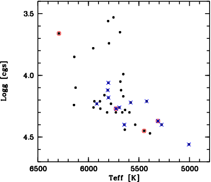
For all our computations we have used 1-D LTE atmosphere models computed with ATLAS9 code by Kurucz 1993; Kurucz 2005. For our program stars we used atmosphere parameters derived by Caffau et al. 2019a with microturbulence velocity of 1 km s-1. The atmospheric parameters , , [Fe/H] are presented in Table 2, where we adopted for the Sun (Caffau et al. 2011). The twelve stars, for which the NLTE abundances were also determined with the help of optical spectra, are marked in Table 2 with asterisks. The lines and atomic data used in the optical investigation of Na, Mg, Al, S, K and Sr for these twelve stars were described in each introductive papers devoted to the NLTE atomic model for each ion. In Fig. 1 the sample of stars is presented in the , plane; the twelve stars above mentioned are highlighted with blue crosses.
In the following sections we shall compare our abundances both with those of Caffau et al. 2019a for the same set of stars and with the abundances of a set of 41 552 stars with stellar parameters similar to our sample extracted from the APOGEE catalogue, SDSS data release 16 (Ahumada et al. 2019). The summary plots of this latter comparison are shown in Fig. 2.

| Star | Teff, K | log g | [Fe/H] | [Na/Fe] | [Mg/Fe] | [Al/Fe] | [S/Fe] | [K/Fe] | [Sr/Fe] |
|---|---|---|---|---|---|---|---|---|---|
| HD 20670 | 5688 | 3.65 | 0.10 | 0.170.10 | 0.110.05 | 0.110.07 | 0.020.06 | 0.050.12 | –0.030.03 |
| HD 24040* | 5809 | 4.12 | 0.09 | 0.090.12 | 0.080.05 | 0.100.10 | –0.040.08 | –0.010.12 | –0.050.02 |
| HD 28005* | 5802 | 4.18 | 0.21 | 0.210.10 | 0.050.07 | 0.100.10 | 0.000.07 | 0.020.12 | –0.080.03 |
| HD 32673 | 5752 | 3.53 | 0.07 | 0.130.10 | 0.160.05 | 0.170.07 | –0.010.07 | 0.030.10 | 0.010.04 |
| HD 34445* | 5803 | 4.06 | –0.03 | 0.130.10 | 0.110.05 | 0.110.10 | 0.070.07 | 0.040.10 | 0.060.03 |
| HD 34575* | 5582 | 4.22 | 0.18 | 0.070.10 | 0.100.06 | 0.070.08 | –0.060.08 | 0.010.12 | –0.050.05 |
| HD 44420 | 5777 | 4.23 | 0.19 | 0.150.13 | 0.020.05 | 0.180.12 | 0.020.10 | 0.020.12 | 0.000.03 |
| HD 56303 | 5941 | 4.21 | 0.05 | 0.020.10 | 0.070.06 | 0.070.08 | –0.020.08 | –0.010.10 | 0.080.04 |
| HD 67346 | 5953 | 3.78 | 0.14 | 0.110.15 | 0.070.06 | 0.070.10 | 0.030.10 | –0.020.10 | 0.070.04 |
| HD 69056 | 5637 | 4.28 | 0.05 | 0.010.10 | 0.100.05 | 0.150.10 | –0.010.10 | 0.040.10 | 0.000.05 |
| HD 69809 | 5842 | 4.16 | 0.17 | 0.130.12 | 0.080.06 | 0.120.08 | 0.010.08 | –0.030.10 | –0.060.03 |
| HD 69960 | 5655 | 3.99 | 0.22 | 0.080.10 | 0.020.06 | 0.080.10 | –0.020.08 | –0.010.10 | –0.080.05 |
| HD 73226 | 5886 | 4.21 | 0.06 | 0.040.12 | 0.030.06 | 0.060.10 | –0.020.07 | 0.010.08 | 0.030.01 |
| HD 73933 | 6143 | 4.24 | 0.06 | -0.080.12 | 0.040.05 | 0.020.10 | –0.030.08 | –0.010.10 | 0.140.06 |
| HD 76909 | 5655 | 4.17 | 0.24 | 0.140.15 | 0.070.07 | 0.070.08 | 0.020.10 | 0.010.10 | 0.000.07 |
| HD 77519 | 6140 | 3.85 | 0.14 | 0.010.12 | 0.080.06 | 0.090.15 | 0.030.12 | –0.010.10 | 0.140.05 |
| HD 82943* | 5917 | 4.23 | 0.13 | 0.100.12 | 0.030.06 | 0.060.10 | 0.000.07 | –0.070.10 | 0.010.04 |
| HD 85301 | 5640 | 4.44 | 0.05 | -0.050.12 | –0.030.04 | –0.040.10 | 0.020.12 | 0.010.08 | 0.190.04 |
| HD 87359* | 5645 | 4.40 | –0.07 | 0.010.10 | 0.100.06 | 0.040.10 | 0.080.07 | 0.010.12 | 0.090.06 |
| HD 87836 | 5684 | 4.05 | 0.16 | 0.220.12 | 0.090.05 | 0.130.10 | 0.020.10 | 0.010.10 | 0.030.05 |
| HD 90681 | 5950 | 4.26 | 0.16 | –0.020.12 | 0.040.06 | 0.050.07 | –0.040.12 | –0.040.10 | –0.020.05 |
| HD 90722 | 5677 | 4.12 | 0.22 | 0.080.12 | 0.040.05 | 0.090.10 | –0.040.10 | –0.020.10 | –0.050.03 |
| HD 92788* | 5694 | 4.26 | 0.13 | 0.150.15 | 0.070.10 | 0.150.10 | 0.060.07 | –0.040.15 | 0.040.05 |
| HD 97645 | 6127 | 4.10 | 0.14 | –0.020.15 | 0.020.04 | 0.090.10 | –0.020.12 | –0.020.12 | 0.060.05 |
| HD 98618* | 5727 | 4.27 | –0.11 | 0.070.08 | 0.080.06 | 0.080.07 | 0.110.08 | 0.000.12 | 0.130.04 |
| HD 98736* | 5276 | 4.40 | 0.29 | 0.170.15 | –0.030.07 | 0.060.10 | –0.040.10 | –0.080.15 | –0.110.08 |
| HD 99491 | 5537 | 4.40 | 0.25 | 0.150.12 | 0.040.07 | 0.140.10 | –0.070.12 | 0.030.12 | –0.060.06 |
| HD 99492* | 5006 | 4.56 | 0.20 | 0.220.12 | 0.000.09 | 0.170.15 | –0.050.12 | –0.030.15 | –0.030.06 |
| HD100069 | 5796 | 3.74 | –0.03 | 0.080.15 | 0.110.08 | 0.130.10 | 0.060.08 | 0.060.12 | 0.090.04 |
| HD105631 | 5391 | 4.47 | 0.05 | –0.010.12 | 0.040.06 | 0.030.08 | 0.030.08 | 0.020.10 | 0.100.04 |
| HD106116 | 5665 | 4.30 | 0.03 | 0.100.10 | 0.050.06 | 0.110.08 | 0.000.08 | 0.040.10 | 0.050.03 |
| HD106156 | 5449 | 4.45 | 0.10 | 0.040.12 | 0.040.08 | 0.050.15 | 0.020.12 | 0.010.08 | 0.010.04 |
| HD108942 | 5882 | 4.27 | 0.20 | 0.080.15 | 0.000.08 | 0.040.10 | –0.090.10 | 0.020.10 | –0.050.06 |
| HD114174 | 5728 | 4.30 | –0.06 | 0.090.10 | 0.080.07 | 0.110.10 | 0.020.10 | 0.070.10 | 0.280.06 |
| HD116321 | 6292 | 3.66 | 0.10 | 0.180.20 | 0.130.04 | 0.200.18 | 0.060.12 | –0.010.12 | 0.170.08 |
| HD136618 | 5805 | 3.56 | 0.14 | 0.180.18 | 0.090.05 | 0.100.12 | –0.030.10 | –0.020.10 | 0.020.05 |
| HD145675* | 5312 | 4.37 | 0.33 | 0.180.15 | 0.060.04 | 0.070.10 | –0.020.09 | –0.030.10 | –0.110.06 |
| HD147231 | 5594 | 4.30 | –0.14 | 0.090.15 | 0.220.09 | 0.090.15 | 0.070.10 | 0.200.12 | 0.050.06 |
| HD159222 | 5815 | 4.30 | 0.00 | 0.050.10 | 0.050.03 | 0.050.10 | 0.040.10 | –0.040.12 | 0.080.06 |
| HD190360* | 5424 | 4.21 | –0.01 | 0.110.12 | 0.170.08 | 0.180.10 | 0.200.09 | 0.080.12 | 0.050.05 |
To estimate the difference in the results between the NLTE and LTE approximations, for four representative stars of our sample, we determined the LTE abundances of the studied elements using the same set of lines and the same atomic parameters. The results are given in Table 3, where the LTE [X/Fe] is reported as well as the difference NLTE–LTE abundance (NLTE in the Table). The choice of the four stars was driven by the desire to span the stellar parameter space. In Fig. 1 the selected stars are highlighted (red open circle) over the complete sample in the , space.
| Star | Teff, K | log g | [Fe/H] | [Na/Fe] | NLTE | [Mg/Fe] | NLTE | [Al/Fe] | NLTE | |||
|---|---|---|---|---|---|---|---|---|---|---|---|---|
| HD98618 | 5727 | 4.27 | –0.11 | 0.090.09 | 0.04 | –0.02 | 0.120.07 | 0.04 | –0.04 | 0.130.09 | 0.06 | –0.05 |
| HD106156 | 5449 | 4.45 | 0.10 | 0.060.14 | 0.07 | –0.02 | 0.080.10 | 0.06 | –0.04 | 0.120.16 | 0.06 | –0.07 |
| HD116321 | 6292 | 3.66 | 0.10 | 0.220.25 | 0.15 | –0.04 | 0.150.06 | 0.04 | –0.02 | 0.260.19 | 0.04 | –0.06 |
| HD145675 | 5312 | 4.37 | 0.33 | 0.210.16 | 0.04 | –0.03 | 0.100.06 | 0.05 | –0.04 | 0.120.11 | 0.03 | –0.05 |
| Star | Teff, K | log g | [Fe/H] | [S/Fe] | NLTE | [K/Fe] | NLTE | [Sr/Fe] | NLTE | |||
| HD98618 | 5727 | 4.27 | –0.11 | 0.140.11 | 0.07 | –0.03 | 0.180.15 | 0.09 | –0.18 | 0.410.05 | 0.03 | –0.28 |
| HD106156 | 5449 | 4.45 | 0.10 | 0.040.14 | 0.04 | –0.02 | 0.180.14 | 0.12 | –0.17 | 0.250.05 | 0.03 | –0.24 |
| HD116321 | 6292 | 3.66 | 0.10 | 0.140.18 | 0.13 | –0.08 | 0.200.18 | 0.13 | –0.21 | 0.620.09 | 0.03 | –0.45 |
| HD145675 | 5312 | 4.37 | 0.33 | 0.000.10 | 0.04 | –0.02 | 0.110.14 | 0.10 | –0.14 | 0.070.07 | 0.04 | –0.18 |
Notes: – the additional error introduced by the use of LTE approximation.
2.1 NaI
The NLTE sodium model atom was first described in Korotin & Mishenina 1999 and later updated by Dobrovolskas et al. 2014. This model provides the NLTE solar sodium abundance A(Na)=6.25, derived from optical lines and reported in Table 1. The oscillator strengths for the 1074.6–1267.9 nm lines were taken from Wiese et al. 1969, for the 2205.6 and 2208.3 nm lines from McEachran & Cohen 1983, and for the 2334.8–2337.9 nm lines from the NIST database (Reader et al. 2012).
The theoretical NLTE synthesis of the 996.1 nm line cannot reproduce the observed solar spectrum, as well as the 2145.2 nm line. The problem is that these observed lines are weaker than in the theoretical synthesis. The estimated NLTE effects cannot explain such a difference, therefore those lines were excluded from the analysis.
For all the lines (except one at 1267.9 nm) we took van der Waals parameter: = –7.06 (hereafter we use as a of the line FWHM per perturber at K in units). This value is slightly larger than the estimated value from Unsöld’s formula (Unsöld 1955) but it provides a better fit with observed solar profile.
For the atomic model of sodium, as well as for the other models considered here, we must make the following remark. Correction of , if necessary, is performed only for lines with developed wings. For such lines, the influence from the accepted value of is higher than from the uncertainty of the oscillator strength (the latter possibility, of course, is not excluded). Such line profiles cannot be adjusted only by changing the element abundance or the value of .
Below we list some notes on individual lines when comparing the NLTE theoretical synthesis to the observed solar spectrum.
- •
The synthesis of the line at 1074.644 nm reproduces very well the observed solar spectrum.
- •
The lines at 1083.484, 1083.484, 1083.490 nm give abundances by about 0.1 dex lower than our adopted solar sodium abundance.
- •
The lines at 1267.917, 1267.917, and 1267.922 nm give abundance by 0.05 dex higher than our NLTE solar sodium abundance. for these lines was taken from Barklem et al. 2000.
- •
For three lines (2205.640, 2208.366 and 2334.837 nm) the agreement between the NLTE theoretical synthesis and the solar observed spectrum is very good, while in the two lines at 2337.896 and 2337.914 nm a higher solar abundance (by 0.04 dex) would be needed to reproduce the solar observed spectrum.
- •
All the lines are formed practically in LTE (EWs vary in the range from –2% to +4%).
- •
The exception is multiplet 2334.8–2337.9 nm whose lines in NLTE are strengthened by about 7–15%.
It is possible that a deviation within 0.1 dex of the sodium content obtained from the individual lines listed above from the adopted solar sodium abundance of Table 1 may be due to inaccuracy of our adopted oscillator strengths. An investigation of this issue is beyond the scope of this work. Similar conclusion can also be applied to some lines of other ions, discussed below.
Our NLTE abundance of sodium in the program stars differ from LTE abundances obtained by Caffau et al. 2019a from 0 to 0.25 dex. On average, our NLTE abundance is 0.09 dex higher than the LTE abundance of Caffau et al. 2019a. We should stress that this comparison is not just as NLTE – LTE difference because the lines used are not the same and the atomic parameters used neither.
The relative abundance [Na/Fe] of our sample stars shows a weak trend with metallicity, the effect is an increase with increasing metallicity (the range is from –0.08 to 0.22 dex). A non parametric test with Kendall’s provides in fact a correlation probability of 99%. The same test on the subset of 1 679 stars with Na measurements shows also a 99% probability of correlation. If we divide the two samples in 0.1 dex metallicity bins the GIANO sample has in each bin that ranges from 0.007 dex to 0.080 dex. For the APOGEE sample it ranges from 0.27 dex to 0.36 dex. The mean abundance for the 40 stars is [Na/Fe] = +0.09 0.07. It should be noted that the abundance from IR lines agrees well with abundance derived from optical lines (the mean deviation is only +0.03 dex). Individual deviations do not exceed dex.
In Appendix (Fig. 10) we show some examples of the observed and synthetic NLTE and LTE profiles of two sodium lines in the solar and stellar observed spectra. Fig. 3 shows the derived NLTE sodium abundances for our sample of stars vs. [Fe/H] and [Mg/H] (-element). The A(Fe) determination is from Caffau et al. 2019a, so it is in LTE while the A(Mg) is the value here derived in NLTE. We understand the inconsistency in mixing LTE and NLTE abundances, but still we think useful to provide, for each element, [X/Fe] versus [Fe/H], which is what usually presented in the literature.
The NLTE effects for Na in this stellar parameter space are well within the uncertainties, being for the four representative stars at maximum –0.04 dex.


2.2 MgI
The NLTE magnesium (Mg i) atomic model was described in Mishenina et al. 2004 and later updated by Černiauskas et al. 2017. Our NLTE solar magnesium abundance from optical lines is A(Mg)=7.54 (see Table 1). The oscillator strength for the 1081.12 nm line was taken from Kurucz & Peytremann 1975; for the 1203.9–1208.3 nm lines – from Chang & Tang 1990, and for other lines – from NIST database (the latter uses mainly the results of calculations by Butler, Mendoza & Zeippen 1993). The van der Waals parameters were calculated using Unsöld’s formula and then corrected with the help of lines from solar spectrum. For line at 1182.8 nm we used the value reported in Barklem et al. 2000. NLTE effects lead to the strengthening of the line in vicinity of the core, while the wings remain practically unchanged. The lines at 982.1, 982.8, 998.3, 998.6 nm are formed practically in LTE. To fit the synthetic line profiles to the solar observed ones, by keeping our adopted solar abundance, one needs to increase the oscillator strengths of these lines by about 0.08 dex, which is of the same order of magnitude of the line-to-line scatter for the Mg investigation (see Table 2).
Some comments on the lines here below about the solar study of the Mg lines.
- •
The feature at 1081.1 nm is formed by 8 components. The NLTE corrections are not negligible (exceed 5% in EW). The wings of this feature can be adjusted if is decreased from –6.68 (Barklem et al. 2000) to –6.82 (the value derived from the solar spectrum).
- •
The lines at 1095.3, 1095.7 and 1096.5 nm are formed practically in LTE.
- •
For line at 1182.8 nm the NLTE correction in EW achieves 6%.
- •
The line at 1203.9 nm is formed practically in LTE.
- •
The NLTE effect for the 1208.3 nm feature is modest (about 5% in EW). This feature is a blend of two lines. The wing of this blend can be adjusted if is decreased from –6.98 (Barklem et al. 2000) to –7.12 (from the solar spectrum).
- •
The lines at 1241.7, 1242.3, 1243.3 nm are formed practically in LTE.
- •
The lines at 1502.4, 1504.0, 1504.7 nm show very small NLTE effects.
- •
The lines at 1574.0, 1574.8, 1576.5 nm also show very small NLTE effects.
- •
For the 1710.8 nm line, the NLTE effects are about 5% in EW.
The NLTE correction for Mg for the four selected stars is small, up to –0.04 dex. In Appendix (Fig. 10) we show NLTE and LTE profiles of two magnesium lines in the solar and stellar spectra. Fig. 4 is the same as Fig. 3 but for magnesium.
From our data one can infer a decrease of the [Mg/Fe] ratio with increasing metallicity with a probability of over 99%. Such a decrease is also clear from the APOGEE data, however the decrease is not as steep as in our data. Our [Mg/Fe] ratios are higher than the APOGEE data by about 0.08 dex for the lowest metallicity bin and converge towards the APOGEE values at higher metallicities.

2.3 Al I
The aluminum NLTE atomic model is described in detail in Andrievsky et al. 2008 and Caffau et al. 2019b. Our adopted NLTE solar abundance is A(Al)=6.43 (see Table 1). The van der Waals parameters for the IR lines were obtained from Unsöld’s formula. For some lines the van der Waals parameters were corrected using the solar spectrum. Some details on individual lines while comparing theoretical NLTE profile to the observed solar spectrum are given below.
- •
The line at 1087.297 nm (NIST ) is very well modeled by the synthetic spectrum. This line is formed in LTE.
- •
The line at 1089.174 nm (NIST ) cannot be reproduced by theoretical synthesis. Probably this line is a blend, because its listed in NIST has an accuracy better than 10%. The estimated NLTE correction is negligible for this line.
- •
The theoretical NLTE profile of line at 1312.341 nm ( are from Wiese et al. 1969) reproduces very well the observed solar profile, once the is adjusted. The LTE profile is wider in the wings but shallower in the core compared to observed profile. The NLTE EW in the solar spectrum appears to be somewhat larger but not very significantly (3–5%) with respect to the LTE EW. For the stars this difference can be larger (up to 13 %, which corresponds to 0.15 dex in abundance).
- •
The line at 1315.075 nm ( are from Wiese et al. 1969 and was derived to fit the solar spectrum) is blended in the solar spectrum with a telluric line. However, the profile of this line in the spectra of the studied stars is well described with the same abundance as derived from the 1312.3 nm line. The value of the is taken the same as for the line 1312.3 nm of the same multiplet. Therefore, we can assume that parameters of this line are fairly reliable.
- •
Synthetic profile of the line at 1671.896 nm (NIST and was optimised to reproduce the solar spectrum) is weaker than the observed one. This result cannot be attributed to an inaccuracy in value, since the accuracy on the oscillator strength is better than 3%. The core of the line profile in LTE is shallower than what is calculated in NLTE. In any case NLTE effects are small for this line.
- •
The central part of the line at 1675.056 nm (NIST and was adjusted to fit the solar spectrum) is blended with a telluric line in the solar spectrum. This does not allow us to estimate the accuracy of the value . In the stellar spectra the synthetic profile of this line is systematically weaker than observed one. The difference is not the result of the inaccuracy, since it is better than 3%.
- •
The line at 1676.336 nm (NIST and was adjusted to fit the solar spectrum) is described very well in the solar spectrum. For the stellar spectra the difference LTE and NLTE in EW can achieve up to 4% (which corresponds to 0.05 dex in abundance).
- •
The line at 2109.303 nm ( is from Kurucz & Peytremann 1975) is This does not allow us to check the value of . Therefore, we use the parameter the same as for the line 2116.376 nm of the same multiplet. For the stars, the abundance derived from this line, agrees with abundance derived from the line at 2116.3 nm. LTE profile of this line is shallower than in the observed spectrum. For the Sun, the NLTE EW is slightly larger but insignificantly (3–5 %) than the LTE value. For the stellar spectra this difference can achieve up to 12 %.
- •
The NLTE synthetic profile of the line at 2116.376 nm ( is from Kurucz & Peytremann 1975 and was derived from the solar spectrum) reproduces very well the solar observed spectrum.
In order to derive aluminum abundance in the dwarf stars, using GIANO spectra, we used the following lines: 1087.2, 1312.3, 1315.0, 1671.8, 1676.3, 2109.3, 2116.3 nm. The abundance of aluminum derived from the IR lines is practically the same as from the optical lines at 669.6, 669.8, 736.1, 736.2, 783.5, 783.6, 877.2, 877.3 nm. The difference is no more than 0.04 dex. Our NLTE aluminum abundance differs from LTE abundance derived by Caffau et al. 2019a up to 0.15 dex. The mean difference is about 0.05 dex (our value is lower) but this difference is probably due to the differences in adopted atomic data and lines used.
[Al/Fe] does not show any dependence on metallicity. This value is distributed in the range from –0.05 to 0.20 dex with a mean value from 40 stars [Al/Fe] = +0.09 0.05.
The NLTE correction we derived for the four selected stars is small, on average about –0.06 dex. In Appendix (Fig. 10) we show NLTE and LTE profiles of two aluminum lines in the solar and stellar spectra. Fig. 5 is the same as Fig. 3 but for aluminum.


2.4 S I
The sulfur NLTE model is described in detail in Korotin 2009. For the solar sulfur abundance this model, used in the optical wavelength range, provides A(S)=7.16 (see Table 1). For the lines at 921.2–923.7 nm, the oscillator strengths we applied are from Biemont et al. 1993, as well as for the lines at 2250.0–2270.0 nm. The synthetic profiles of the lines at 1045.5, 1045.6, 1045.9 nm are in good agreement with the solar spectrum when using values from Wiese et al. 1969. Van der Waals parameters for these lines are from Barklem et al. 2000.
For the lines in the region 1540.0–1542.3 nm, the oscillator strengths were taken from two sources: Biemont et al. 1993 and NIST. It should be noted that the from NIST are lower by 0.18 dex with respect to the data of Biemont et al. 1993. The same is valid for the lines of the multiplet at 1546.9–1547.9 nm, where the difference between the is 0.16 dex. The lines at 1540.0, 1540.3 nm are blended with telluric lines in the solar spectrum, therefore we cannot use them to check their parameters. The lines at 1542.3, 1546.9, 1547.5, 1547.8 nm are clean, and we found that their values can be decreased by 0.1 dex (with respect to the data of Biemont et al. 1993) to achieve a good agreement with the observed profiles in the solar spectrum. It is important to note that these lines are weak in the solar spectrum (residual intensity is larger than 0.85), therefore, the influence of the accepted values of on their calculated strength is predominant. Thus, we one can conclude that, most likely, the real values of for mentioned lines appear to be between the data of Biemont et al. 1993 and NIST. The NIST accuracy for these oscillator strengths are %, and they are listed in Table 4. The lines at 2250.7, 2251.9 nm are reproduced with a reasonable agreement in the solar spectrum but the continuum in this region is not quite reliable. The lines at 2255.2, 2256.3, 2257.5, 2264.4 nm are slightly blended with telluric lines in the solar spectrum, and the line at 2270.7 nm is very well reproduced by a synthetic profile.
Actually, in our NLTE analysis of dwarf spectra we used the following lines: 1045.5, 1045.6, 1045.9 nm (principal lines for which NLTE corrections are moderate: EWs are up to 25%, i.e. –0.3 dex in abundance). The NLTE corrections increase as effective temperature increases. For most stars the corrections are within 0.15 dex. The lines at 1540.0–1547.9 nm have the NLTE corrections up to 5% in EW. For these lines, we derive a correction in abundance of +0.10 dex, which can be due to an inaccuracy of the oscillator strengths (see discussion in the beginning of this subsection). The lines at 2250.7, 2251.9, 2255.2, 2257.5, 2256.3, 2264.4, 2270.7 nm are formed almost in LTE (difference in EWs is about 3%).
For our analysis in the optical range we used the following lines: 921.2, 922.8, 923.7 nm (large NLTE corrections: from 0.13 to 0.18 dex), 869.3 and 869.4 nm (corrections are rather small: from 0.05 to 0.03 dex), 674.3, 674.8, 675.7, 605.2 nm (lines are formed almost in LTE). The agreement between the abundances derived from GIANO spectra and the UVES and ESPaDOnS spectra is excellent (within the range of 0.04 dex). Our NLTE sulfur abundances for individual stars differ from LTE values of Caffau et al. 2019a from –0.17 to 0.15 dex and our mean NLTE abundance for all sample of stars is about 0.02 dex lower than the mean LTE value derived by Caffau et al. 2019a, but these comparisons are related to the difference in selected atomic data and lines used, not to NLTE effects. The ratio [S/Fe] demonstrates a prominent increase with metallicity decrease (probabilty over 99%). Such an increase is stastically apparent also in the APOGEE data, however in our data it is considerably steeper, with [S/Fe] ratios higher than in the APOGEE data at the lowest metallicities and lower at the highest metallicity, with a cross-over at about 0.1 dex. The ratios for individual stars are within the interval from –0.09 to 0.20 dex. The mean value from 40 stars is [S/Fe]= +0.010.05.
The sulphur NLTE correction, we derived for the four selected stars, is negligible for the three cooler stars, for the hottest star it is –0.08 dex, but anyway smaller than the line-to-line scatter. In Appendix (Fig. 10) we show NLTE and LTE profiles of two sulfur lines in the solar and stellar spectra. Fig. 6 is the same as Fig. 3 but for sulfur.


2.5 K I
The potassium NLTE atomic model was described in Andrievsky et al. 2010. The basic atomic model was modified: photoionization cross sections for some levels were added following to the data from by Zatsarinny & Tayal 2010; then, for the six lower levels collisional rates with hydrogen atoms were added (Belyaev & Yakovleva 2017). The oscillator strengths for the lines at 1176.9 and 1177.2 nm were taken from Safronova et al. 2013, for other lines – from Wiese et al. 1969. For the lines at 1176.9, 1177.2, 1243.2, 1252.2 nm damping parameters are from Barklem et al. 2000. For the lines at 1516.3 and 1516.8 nm van der Waals parameters were calculated with the help of from Unsöld’s formula. Our solar potassium abundance derived from the optical range is A(K)=5.11 (see Table 1). All potassium lines in the IR domain of the solar spectrum are strengthened due to NLTE effects (abundance corrections are from 0.03 to 0.18 dex).
There are some important details. In the stellar spectra the right wing of the 1176.9 nm line is distorted by CN lines. In the solar spectrum these lines are separated, and potassium line is well reprouced by theoretical synthesis. A telluric absorption blends the 1177.2 nm line in the solar spectrum. The line at 1243.2 nm is well reproduced by the synthetic profile. The left wing of the 1252.2 nm line in the stellar spectra is distorted by the presence of the 1252.181 nm Cr i line, but it is not a problem for the solar spectrum. The line at 1516.3 nm is situated in a telluric absorption wing in the solar spectrum. In the stellar spectra the left wing of this line is distorted by the presence ot the 1516.265 nm CN band. This line is formed in LTE. Similar situation is seen for the 1516.8 nm line, which is also blended by a telluric line, and formed in LTE. The right wing of this line in the stellar spectra is distorted by the 1516.866 nm CN band and the 1516.887 nm Fe i line.
For the stellar spectra we used as a rule the 1176.9, 1177.2, 1243.2, 1252.2 nm lines. The lines at 1516.3 and 1516.8 nm were used as auxiliary lines (since they are partially blended with CN bands). In order to compare the abundances from GIANO to those derived from UVES and ESPaDOnS, we used the 766.4 and 769.8 nm lines. We found that the differences in abundances are within 0.05 dex. Only for one star, HD98736, the difference was 0.11 dex (the abundance from IR lines is higher). The difference of the mean abundances from NLTE analysis and LTE analysis by Caffau et al. 2019a is up to 0.3 dex; in this difference the NLTE effects play a part but the difference is also related to atomic data choice. [K/Fe] vs. [Fe/H] shows a small increase of the potassium abundance as metallicity decreases, this is statistically significant (99.7%). A similar increase is statistically apparent also in the APOGEE data, although impossible to detect visually, even after binning the data in metallicity.The mean potassium abundance based on the 40 stars is [K/Fe] = +0.010.05.
The NLTE correction, we derived for the four selected stars, is not negligible; it is comparable to or slightly larger than the uncertainty on the abundance determination. In Appendix (Fig. 10) we show NLTE and LTE profiles of two potassium lines in the solar and stellar spectra. Fig. 7 is the same as Fig. 3 but for potassium.


2.6 Sr II
The strontium NLTE atomic model is from Andrievsky et al. 2011. Our solar strontium abundance derived from the solar optical spectrum is A(Sr)=2.92 (see Table 1). Synthetic spectra of the three lines at 1003.6, 1032.7, 1091.4 nm ( are from Warner 1968 and are from Barklem et al. 2000) are able to well reproduce the solar observed spectrum. We found that NLTE effects strongly influence these lines. As a rule, the line EWs in the solar spectrum are increased by 20–25%, but in some cases the NLTE corrections achieve about 0.20–0.36 dex. The mean NLTE abundance differs from the LTE abundance published by Caffau et al. 2019a by about 0.5 dex. Surely, in this difference the NLTE plays a big role. The [Sr/Fe] ratio shows a clear dependence on [Fe/H]: the lower the metallicity, the larger the [Sr/Fe] ratio. When [Fe/H]=+0.10, [Sr/Fe] equals to zero.
The NLTE correction, we derived for the four selected stars, is in the range from –0.18 (for the coolest star) to –0.45 (for the hottest star). Being the uncertainty on the abundance determination small (always within 0.1 dex), for these Sr lines the NLTE effect should be taken into account, when possible. In Appendix (Fig. 10) we show NLTE and LTE profiles of two strontium lines in the solar and stellar spectra. Fig. 8 is the same as Fig. 3 but for strontium.


3 Discussion
The main goal of this investigation was to provide, for Na i, Al i, Mg i, S i, K i and Sr ii, a list of lines in the IR wavelength range that can be safely used in an LTE investigation. The selected lines, covering the complete wavelength range of GIANO (950–2450 nm), are listed in Table 4. In the Table we provide the oscillator strength, the and a comment on the line: LTE means the line can safely be analysed in the LTE approximation (absolute NLTE correction is smaller than 0.02 dex), while NLTE means that the line is affected by departure from LTE. For a few lines the string “small NLTE” means that there is a minor NLTE effect (not larger than 5% in EW). These computations can safely be applied for unevolved, solar-metallicity stars, with stellar parameters similar to the sample here analysed (see Fig 1). Clearly, in another parameter space NLTE effects can be different. In Fig. 10 for a few selected lines the observed profiles of the Sun and of the three stars (HD 20670, HD 24040 and HD 114174) are compared to the LTE and NLTE theoretical profiles. As one can see, the agreement of NLTE synthetic profile with the observed spectrum is very good, while for several cases the theoretical LTE profile deviates from the observation.
The trends of the investigated elements as a function of the metallicity confirm the ones that are apparent from the APOGEE data, although there are some minor differences in the slopes for Na, Mg and S.
- •
Na. In the upper panel of Fig. 3, [Na/Fe] is plotted as a function of [Fe/H], using Fe as a proxy for metallicity. The four stars with an LTE analysis (open symbols in the figure, connected with a line to the NLTE result) show the small NLTE effects for this parameters space. In fact, of the twelve Na i lines investigated, only three are sensitive to NLTE (see Table 4). In the lower panel of the same figure, Mg is used as a proxy for the metallicity, taking the advantage of a more coherent picture because both Na and Mg are investigated in NLTE. In both panels, a relative increase in the ratio of Na over metallicity at increased metallicity is visible. In Fig. 9 the analysis here done is compared to the analysis by Caffau et al. 2019a on the same stars. The average difference from the two investigations is 0.09 dex, ranging from about zero to 0.25 dex. This difference is not due to NLTE effects (which is of the order of 0.03 dex), but to the adjustment of the atomic data on the solar spectrum done here and not in Caffau et al. 2019a. Surely with this new analysis the scatter star-to-star is smaller. Summarizing, a great majority of sodium lines in the wide range of effective temperature from 5000 to 6500 K and sodium relative abundances [Na/H] from –0.8 to +0.8 are insensitive to the deviation from LTE. This is valid for the dwarfs, but for the stars with less than 3 one needs to apply the deatiled NLTE calculatins.

Figure 9: Relative sodium abundances ([Na/Fe] versus [Fe/H] from this analysis (filled circles) compared to the results of analysis Caffau et al. 2019a (open tiangles). - •
Mg. As visible in Fig. 4 and in Table 3, the NLTE effects for Mg are tiny. Of the 26 Mg i lines (the eight components of 1081.1 nm we considered as a single line) investigated, four are sensitive to NLTE (see Table 4). As visible from the Figure, there is an evident trend of the [Mg/Fe] to decreasing at increasing metallicity. In general, in the effective temperature range from 5200 to 6500 K the NLTE effects are the same as previously described (for relative magnesium abundance [Mg/H] from –0.7 to +o.7). However, the deviations increase for the giant stars with less than 2.5.
- •
Al. From the upper panel of Fig. 5, one can see a flat [Al/Fe] versus [Fe/H], while on the lower panel, there is a hint for an incresing [Al/Fe] for increasing [Mg/Fe]. The NLTE effects on the Al i lines are about 0.05 dex (see Table 3), smaller than the line-to-line scatter for all stars. The nine Al i lines here analyzed suffer all but one from NLTE effects, which are anyway not strong. The mean difference from the analysis of Caffau et al. 2019a is 0.05 dex, with a few cases with differences up to 0.15 dex that are due to atomic data and line selection. As a concluding remark it can be noted that two Al i lines 1087.2 and 1089.1 nm can be safely used in LTE analysis for the dwarfs stars with larger than 3 and affective temperature lower than 6000 K (for the wide range of the relative aluminum abundances from –0.7 to +0.7). At the same time for the subgiant and giant stars, as well as for hotter dwarfs the detailed NLTE calculations are necessary.
- •
S. In the upper panel of Fig. 6, the decrease of [S/Fe] with increasing metallicity typical in the -elements, is well evident. In the lower panel of Fig. 6, an almost flat [S/Mg] as a function of [Mg/Fe] as a proxy for metallicity is expected because both Mg and S are -elements. The behaviour was very similar in Caffau et al. 2019a, also if single stars could differ up to 0.17 dex, due to choice of the lines, atomic data, but also NLTE for the lines belonging to the multiplet 3. Nineteen lines of S i have been analyzed (see Table 4). Only the three lines belonging to the multiplet 3 (the three bluest lines here analyzed) are strongly affected by NLTE; the other lines are either well represented in LTE or slightly affected by NLTE. The lines of multiplet 3 are the strongest and sometimes the only possibility to derive A(S) in metal-poor stars. The global NLTE effects on the abundance determination for S is small (up to –0.08, see Table 3) because all the S i lines, but the three of multiplet 3, form in conditions close to LTE. Speaking of sensitivity to atmosphere parameters, one can note that seven S i lines at 2250.7–2270.7 nm show the weak influence from the NLTE effects if we are considering the dwarfs with greater than 3 and effective temperatures lower than 6400 K (relative sulfur abundance is from –0.7 to +0.7). NLTE effects are becoming remarkable for the subgiant and giant stars. The same is true for the metal-deficient stars ([Fe/H] –0.7).
- •
K. From both panels of Fig. 7, one can see a decreasing [K/Fe] for increasing metallicity. Of the seven K i lines here analyzed, four are affected by NLTE (see Table 4). The NLTE correction for the stars listed in Table 3 is larger than the line-to-line scatter and the large difference of the LTE and NLTE abundance is evident in Fig. 7. The difference with the analysis by Caffau et al. 2019a is large, certainly affected by the NLTE. Our recommendation for the use of potassium lines depending on the parameters of stellar atmospheres is as follows: lines at 1516.3–1516.8 nm are available for use in the LTE approximation for stars with 3.5 and [K/H] from –0.7 to +0.7. The effective temperature has almost no effect on the NLTE corrections for these lines.
- •
Sr. Fig. 8 shows a decrease of [Sr/Fe] or [Sr/Mg] for increasing metallicity. The three lines here analyzed are strongly affected by NLTE (see Table 4) and the NLTE corrections for the stars with both LTE and NLTE analysis are much larger than the line-to-line scatter and can be up to 0.45 dex (see Table 3).
Concluding our discussion, we should make the following remark: we recommend using certain infrared lines to obtain elemental abundances in LTE, while at the same time leaving open questions about the effect of the limitations of our approach, such as the 1-D approximation, on the obtained abundances.
4 Conclusion
We analyzed IR lines of several ions in the solar spectrum and in the spectra of 40 dwarf stars observed with GIANO spectrograph. We have studied in detail the influence of the NLTE effects on the lines under consideration, and we give our recommendation on which lines can be used to obtain abundance in the LTE approximation, and which lines require NLTE processing. This information is given in the Table 4 in the Appendix.
The sample here discussed is small in size, but has a high quality of the spectra, both in terms of S/N ratio and resolution. It is interesting to note how such a small size sample allows to derive reliable abundance trends that become apparent only for samples that are several orders of magnitude larger in size, but of lower quality, like the APOGEE sample.
Acknowledgements
We would like to thank the referee of this paper for his/her valuable comments.
References
- Ahumada et al. (2019) Ahumada, R., Allende Prieto, C., Almeida, A., et al. 2019, arXiv e-prints, arXiv:1912.02905
- Allende Prieto et al. (2008) Allende Prieto, C., Majewski, S. R., Schiavon, R., et al. 2008, Astronomische Nachrichten, 329, 1018
- Andrievsky et al. (2008) Andrievsky, S. M., Spite, M., Korotin, S. A., et al. 2008, A&A, 481, 481
- Andrievsky et al. (2010) Andrievsky, S. M., Spite, M., Korotin, S. A., et al. 2010, A&A, 509, A88
- Andrievsky et al. (2011) Andrievsky, S. M., Spite, F., Korotin, S. A., et al. 2011, A&A, 530, A105
- Arenou et al. (2018) Arenou, F., Luri, X., Babusiaux, C., et al. 2018, A&A, 616, A17
- Barklem et al. (2000) Barklem, P. S., Piskunov, N., & O’Mara, B. J. 2000, A&AS, 142, 467
- Belokurov et al. (2018) Belokurov, V., Erkal, D., Evans, N. W., et al. 2018, MNRAS, 478, 611
- Belyaev & Yakovleva (2017) Belyaev, A. K., & Yakovleva, S. A. 2017, A&A, 606, A147
- Biemont et al. (1993) Biemont, E., Quinet, P., & Zeippen, C. J. 1993, A&AS, 102, 435
- Butler, Mendoza & Zeippen (1993) Butler K., Mendoza C., Zeippen C. J., 1993, JPhB, 26, 4409
- Caffau et al. (2011) Caffau, E., Ludwig, H.-G., Steffen, M., et al. 2011, Sol. Phys., 268, 255
- Caffau et al. (2019a) Caffau, E., Bonifacio, P., Oliva, E., et al. 2019a, A&A, 622, A68
- Caffau et al. (2019b) Caffau, E., Monaco, L., Bonifacio, P., et al. 2019b, A&A, 628, A46
- Carlsson (1986) Carlsson, M. 1986, Uppsala Astronomical Observatory Reports, 33
- Černiauskas et al. (2017) Černiauskas, A., Kučinskas, A., Klevas, J., et al. 2017, A&A, 604, A35
- Chang & Tang (1990) Chang T. N., Tang X., 1990, J. Quant. Spectrosc. Radiative Transfer, 43, 207
- Cirasuolo et al. (2014) Cirasuolo, M., Afonso, J., Carollo, M., et al. 2014, Proc. SPIE, 9147, 91470N
- Dalton et al. (2018) Dalton, G., Trager, S., Abrams, D. C., et al. 2018, Proc. SPIE, 107021B
- de Jong et al. (2019) de Jong, R. S., Agertz, O., Berbel, A. A., et al. 2019, The Messenger, 175, 3
- Di Matteo et al. (2019) Di Matteo, P., Haywood, M., Lehnert, M. D., et al. 2019, A&A, 632, A4
- Dobrovolskas et al. (2014) Dobrovolskas, V., Kučinskas, A., Bonifacio, P., et al. 2014, A&A, 565, A121
- Gaia Collaboration et al. (2018b) Gaia Collaboration, Brown, A. G. A., Vallenari, A., et al. 2018, A&A, 616, A1
- Gilmore et al. (2012) Gilmore, G., Randich, S., Asplund, M., et al. 2012, The Messenger, 147, 25
- Hase et al. (2010) Hase, F., Wallace, L., McLeod, S. D., et al. 2010, J. Quant. Spectrosc. Radiative Transfer, 111, 521
- Haywood et al. (2018) Haywood, M., Di Matteo, P., Lehnert, M. D., et al. 2018, ApJ, 863, 113
- Helmi et al. (2018) Helmi, A., Babusiaux, C., Koppelman, H. H., et al. 2018, Nature, 563, 85
- Kaeufl et al. (2004) Kaeufl, H.-U., Ballester, P., Biereichel, P., et al. 2004, Proc. SPIE, 1218
- Korotin et al. (1999) Korotin, S. A., Andrievsky, S. M., & Luck, R. E. 1999, A&A, 351, 168
- Korotin & Mishenina (1999) Korotin, S. A., & Mishenina, T. V. 1999, Astronomy Reports, 43, 533
- Korotin (2009) Korotin, S. A. 2009, Astronomy Reports, 53, 651
- Kurucz & Peytremann (1975) Kurucz R. L., Peytremann E., 1975, SAOSR
- Kurucz et al. (1984) Kurucz, R. L., Furenlid, I., Brault, J., et al. 1984, National Solar Observatory Atlas
- Kurucz (1993) Kurucz, R. 1993, ATLAS9 Stellar Atmosphere Programs and 2 km/s grid. Kurucz CD-ROM No. 13. Cambridge, 13
- Kurucz (2005) Kurucz, R. L. 2005, Memorie della Societa Astronomica Italiana Supplementi, 8, 14
- Livingston & Wallace (1991) Livingston, W., & Wallace, L. 1991, NSO Technical Report
- McEachran & Cohen (1983) McEachran, R. P. & Cohen, M. 1983, J. Phys. B:, 16, 3125
- Mishenina et al. (2004) Mishenina, T. V., Soubiran, C., Kovtyukh, V. V., et al. 2004, A&A, 418, 551
- Nissen & Schuster (2011) Nissen, P. E., & Schuster, W. J. 2011, A&A, 530, A15
- Nissen & Schuster (2010) Nissen, P. E., & Schuster, W. J. 2010, A&A, 511, L10
- Origlia et al. (2014) Origlia, L., Oliva, E., Baffa, C., et al. 2014, Proc. SPIE, 914461E
- Quirrenbach et al. (2014) Quirrenbach, A., Amado, P. J., Caballero, J. A., et al. 2014, Proc. SPIE, 91471F
- Reader et al. (2012) Reader, J., Kramida, A., & Ralchenko, Y. 2012, American Astronomical Society Meeting Abstracts #219 219, 443.01
- Reiners et al. (2016) Reiners, A., Mrotzek, N., Lemke, U., et al. 2016, A&A, 587, A65
- Rayner et al. (2016) Rayner, J.T., Tokunaga, A., Jaffe, D. et al., 2016, Proc. SPIE, 9908, id.99088417
- Ryabchikova et al. (2015) Ryabchikova, T., Piskunov, N., Kurucz, R. L., et al. 2015, Phys. Scr., 90, 054005
- Safronova et al. (2013) Safronova, M. S., Safronova, U. I., & Clark, C. W. 2013, Phys. Rev. A, 87, 052504
- Tsymbal (1996) Tsymbal, V. 1996, M.A.S.S., Model Atmospheres and Spectrum Synthesis, 198
- Unsöld (1955) Unsöld, A. 1955, Physik der Stern Atmospharen, Berlin
- Warner (1968) Warner, B. 1968, MNRAS, 139, 115
- Weinberg et al. (2019) Weinberg, D. H., Holtzman, J. A., Hasselquist, S., et al. 2019, ApJ, 874, 102
- Wiese et al. (1969) Wiese, W. L. and Smith, M. W. and Miles, B. M. 1969, Atomic transition probabilities, Vol.2, NSRDS-NBS, Washington, D.C.
- Zatsarinny & Tayal (2010) Zatsarinny, O., & Tayal, S. S. 2010, Phys. Rev. A, 81, 043423
Appendix A


| ,Å | LTE/NLTE | ,Å | LTE/NLTE | ||||
|---|---|---|---|---|---|---|---|
| Na I | Al I | ||||||
| 10746.45 | –1.29 | –7.06 | LTE | 10872.97 | –1.33 | –7.19 | LTE |
| 10834.85 | –0.50 | –7.06 | LTE | 10891.74 | –1.03 | –7.19 | LTE |
| 10834.85 | –1.80 | –7.06 | LTE | 13123.41 | 0.27 | –7.10 | NLTE |
| 10834.91 | –0.66 | –7.06 | LTE | 13150.75 | –0.03 | –7.10 | NLTE |
| 12679.17 | –0.04 | –6.65 | LTE | 16718.96 | 0.22 | –7.16 | NLTE |
| 12679.17 | –1.34 | –6.65 | LTE | 16750.56 | 0.47 | –7.16 | NLTE |
| 12679.22 | –0.20 | –6.65 | LTE | 16763.36 | –0.48 | –7.16 | small NLTE |
| 22056.40 | 0.29 | –7.06 | LTE | 21093.03 | –0.31 | –6.90 | NLTE |
| 22083.66 | –0.01 | –7.06 | LTE | 21163.76 | –0.01 | –6.90 | NLTE |
| 23348.38 | 0.28 | –7.06 | NLTE | ||||
| 23378.96 | –0.42 | –7.06 | NLTE | S I | |||
| 23379.14 | 0.54 | –7.06 | NLTE | 10455.45 | 0.25 | –7.32 | NLTE |
| 10456.76 | –0.45 | –7.32 | NLTE | ||||
| Mg I | 10459.41 | 0.03 | –7.32 | NLTE | |||
| 9983.19 | –2.15 | –7.01 | LTE | 15400.08 | 0.45 | –7.31 | small NLTE |
| 9986.48 | –1.68 | –7.01 | LTE | 15403.72 | –0.28 | –7.31 | small NLTE |
| 9993.21 | –1.45 | –7.01 | LTE | 15403.79 | 0.63 | –7.31 | small NLTE |
| 10811.05 | 0.02 | –6.82 | NLTE | 15422.20 | –1.82 | –7.31 | small NLTE |
| 10811.08 | –0.14 | –6.82 | NLTE | 15422.26 | –0.28 | –7.31 | small NLTE |
| 10811.10 | –1.04 | –6.82 | NLTE | 15422.28 | 0.79 | –7.31 | small NLTE |
| 10811.12 | –1.04 | –6.82 | NLTE | 15469.82 | –0.15 | –7.40 | small NLTE |
| 10811.14 | –2.59 | –6.82 | NLTE | 15475.62 | –0.62 | –7.40 | small NLTE |
| 10811.16 | –0.30 | –6.82 | NLTE | 15478.48 | 0.08 | –7.40 | small NLTE |
| 10811.20 | –0.19 | –6.82 | NLTE | 22507.56 | –0.48 | –7.61 | LTE |
| 10811.22 | –1.28 | –6.82 | NLTE | 22519.07 | –0.25 | –7.61 | LTE |
| 10953.32 | –0.86 | –6.78 | LTE | 22552.57 | –0.04 | –7.61 | LTE |
| 10957.28 | –0.99 | –6.78 | LTE | 22563.83 | –0.26 | –7.61 | LTE |
| 10957.30 | –0.51 | –6.78 | LTE | 22575.39 | –0.73 | –7.61 | LTE |
| 10965.39 | –2.16 | –6.78 | LTE | 22644.06 | –0.34 | –7.61 | LTE |
| 10965.41 | –0.99 | –6.78 | LTE | 22707.74 | 0.44 | –7.61 | LTE |
| 10965.45 | –0.24 | –6.78 | LTE | ||||
| 11828.17 | –0.33 | –7.19 | NLTE | K I | |||
| 12039.82 | –1.53 | –7.22 | LTE | 11769.64 | –0.48 | –7.33 | NLTE |
| 12083.28 | –0.79 | –7.12 | NLTE | 11772.84 | 0.47 | –7.33 | NLTE |
| 12083.65 | 0.41 | –7.12 | NLTE | 12432.27 | –0.43 | –7.02 | NLTE |
| 12417.94 | –1.66 | –7.15 | LTE | 12522.13 | –0.13 | –7.02 | NLTE |
| 12423.03 | –1.19 | –7.15 | LTE | 15163.07 | 0.63 | –7.31 | LTE |
| 12433.45 | –0.97 | –7.15 | LTE | 15163.07 | –0.67 | –7.31 | LTE |
| 15025.00 | 0.36 | –7.05 | small NLTE | 15168.38 | 0.48 | –7.31 | LTE |
| 15040.25 | 0.14 | –7.05 | small NLTE | ||||
| 15047.71 | –0.34 | –7.05 | small NLTE | Sr II | |||
| 15740.71 | –0.21 | –6.95 | small NLTE | 10036.65 | –1.31 | –7.63 | NLTE |
| 15748.89 | –0.34 | –6.95 | small NLTE | 10327.31 | –0.35 | –7.63 | NLTE |
| 15748.99 | 0.14 | –6.95 | small NLTE | 10914.88 | –0.64 | –7.63 | NLTE |
| 15765.65 | –1.51 | –6.95 | small NLTE | ||||
| 15765.75 | –0.34 | –6.95 | small NLTE | ||||
| 15765.84 | 0.41 | –6.95 | small NLTE | ||||
| 17108.63 | 0.06 | –6.98 | NLTE |