A Deep Learning Framework for Hybrid Beamforming Without Instantaneous CSI Feedback
Abstract
Hybrid beamformer design plays very crucial role in the next generation millimeter-wave (mm-Wave) massive MIMO (multiple-input multiple-output) systems. Previous works assume the perfect channel state information (CSI) which results heavy feedback overhead. To lower complexity, channel statistics can be utilized such that only infrequent update of the channel information is needed. To reduce the complexity and provide robustness, in this work, we propose a deep learning (DL) framework to deal with both hybrid beamforming and channel estimation. For this purpose, we introduce three deep convolutional neural network (CNN) architectures. We assume that the base station (BS) has the channel statistics only and feeds the channel covariance matrix into a CNN to obtain the hybrid precoders. At the receiver, two CNNs are employed. The first one is used for channel estimation purposes and the another is employed to design the hybrid combiners. The proposed DL framework does not require the instantaneous feedback of the CSI at the BS. We have also investigated the online deployment of DL for channel estimation. We have shown that the proposed approach has higher spectral efficiency with comparison to the conventional techniques. The trained CNN structures do not need to be re-trained due to the changes in the propagation environment such as the deviations in the number of received paths and the fluctuations in the received path angles up to 4 degrees. Also, the proposed DL framework exhibits at least 10 times lower computational complexity as compared to the conventional optimization-based approaches.
Index Terms:
Deep learning, online learning, channel estimation, hybrid precoding, instantaneous feedback.I Introduction
Millimeter wave (mm-Wave) systems provide higher data rates, larger bandwidth and higher spectral efficiency as compared to the conventional cellular communications [1]. Hence, they become a promising candidate for the fifth generation (5G) wireless communication systems [1, 2, 3]. Compared to sub-6 GHz transmissions envisaged in 5G, the mm-Wave signals encounter a more complex propagation environment characterized by higher scattering, severe penetration losses, lower diffraction, and higher path loss for fixed transmitter and receiver gains [4, 5, 6]. The mm-Wave systems leverage large-scale antenna arrays to compensate the propagation losses at high frequencies. However, the large number of antennas and high power consumption bring the difficulty of using a dedicated RF (radio frequency) chain for each antenna. In order to tackle this problem, hybrid (analog and baseband) beamforming architectures are introduced where small number of phase-only analog beamformers are used to steer the beams and process the down-converted signal via baseband beamformers, each of which is dedicated to a single RF chain [4, 5, 6, 7].
Hybrid beamforming is an effective approach to be used in mm-Wave systems, increasing the spectral efficiency and reduce the cost that could be imposed by large number of antennas in massive multiple-input multiple-output (MIMO) systems [8, 6]. In the literature, different approaches are proposed to design the hybrid beamformers in mm-Wave massive MIMO systems. One basic approach is selecting the columns of the RF precoder and combiners from a predefined codebook, which includes the array responses of receive/transmitted path angles. [6, 9, 10]. However, the determination of the received path angles is very difficult in mm-Wave channel. To overcome this difficulty, phase extraction-based hybrid beamforming (PE-HB) techniques is proposed [11, 10] without requiring such a codebook. In order to obtain an optimum solution, manifold optimization (MO) approach is proposed in [12] where the Euclidean distance between the unconstrained beamformers and the hybrid beamformers (i.e., the multiplication of analog and baseband beamformer) is minimized.
Most of the above techniques assume that the instantaneous channel state information (CSI) is known a priori when designing the hybrid beamformers. Furthermore, the performance of these works strongly relies on the perfectness of the channel [13, 14, 15]. In practice, the pilot signals are periodically transmitted and the received data is processed to obtain the CSI [13]. Hence, it is very crucial to perform channel estimation accurately, especially in the presence of the challenges such as high data rate and short coherence intervals [16]. In order to cope with these challenges, statistical hybrid beamforming (SHB) architectures are proposed where the beamformers are designed by utilizing the channel statistics [17, 18, 19, 20]. In this case, usually the second order statistics, i.e., the channel covariance matrices (CCMs) are used. Via CCM acquisition, the base station (BS) only knows the channel statistics, with infrequent channel information feedback, but no instantaneous CSI feedback. Hence, lower feedback overhead is achieved. In previous works, covariance-based beamforming is considered, for instance in [17, 18], baseband-only beamforming is proposed where the receiver is assumed to have perfect CSI. Hybrid architectures with CCM is considered in [19, 20]. In particular, [19] studies only the hybrid precoder design (without combiners) and [20] assumes the perfect CSI at the receiver, similar to [17, 18]. Furthermore, [20] designs the analog precoders by simply taking the phases of the unconstrained precoders, which is a sub-optimum approach.
In order to obtain low-complexity and effective hybrid beamforming performance, there is a need to design hybrid beamformers without perfect CSI assumption. This motivates us to develop a hybrid beamforming algorithm using channel statistics at the BS without the requirement of the perfect CSI at the receiver. To further obtain robust performance against the estimated/corrupted channel data, we design the hybrid beamformers via a deep learning (DL) approach. DL has attracted many researchers in both communications and signal processing society due to its promising performance against many challenging problems such as channel estimation [21, 22, 23, 24, 25], hybrid beamforming [26, 27, 28, 29, 30]. In particular, multilayer perceptrons (MLPs) have been proposed for hybrid precoding in [26] and [27]. The authors in [27] proposed a coordinated beam training approach via MLPs. In a recent work [24], convolutional neural network (CNN) is designed for channel estimation. In [28], a CNN is designed for joint hybrid precoder and combiner design. A twin-CNN architecture is proposed in [29] for joint antenna selection and hybrid beamforming, and multi-user hybrid beamforming is studied in [30] for mm-Wave massive MIMO systems. Note that the above DL-based beamforming approaches [26, 27] assume the perfect CSI to solve the hybrid beamformer design problem, even if this necessity is relaxed in [28, 29, 30] such that acceptable system rate performance can be achieved with corrupted/imperfect CSI via DL. Thus, driven by the advantages of DL such as its provided low computational complexity and robustness against corrupted input data, we develop a DL framework for the hybrid beamformer design.
In this paper, we introduce a DL framework where hybrid precoding/combining and channel estimation stages, which are very crucial tasks in mm-Wave communication systems, are performed via deep networks (Please see Fig. 2). We design three deep networks for this purpose. At the BS, a deep network called CovNet is used which accepts the input as the CCM and yields the hybrid precoders at the output. At the mobile station (MS), there are two deep networks, namely, ChannelNet and BFNet. ChannelNet is used in the channel training state to estimate the instantaneous CSI. The estimated channel matrix is then fed to BFNet to design the hybrid combiner weights at the output. As a result, the whole DL framework does not require either instantaneous CSI feedback or the perfect CSI at the receiver.
The proposed DL framework has two stages: training (offline) and prediction (online). During training, several received pilot signals, channel and covariance realizations are generated, and hybrid beamforming problem is solved via manifold optimization (MO) approach [12, 31] to obtain the network labels. In the prediction stage, when the CNNs operate online, we estimate the hybrid beamformers and the channel matrix by simply feeding the CNNs with the related input data. The proposed approach is advantageous since it does not require the perfect channel data in the prediction stage and still provides robust performance. We summarize the main contributions of this paper as follows.
- 1.
A DL framework is proposed which solves the hybrid beamformer design without instantaneous CSI feedback and does not require the perfect CSI at the receiver. Due to infrequent feedback of channel information, the proposed method has lower feedback overhead as compared to the conventional approaches [6, 9, 10, 11, 12, 10].
- 2.
- 3.
- 4.
- 5.
We have investigated the online deployment of the proposed DL-based channel estimation scheme where the deep network adapts itself to the propagation environment.
Notation: Throughout the paper, vector and matrix quantities are denoted by boldface lower and upper case symbols, respectively. In the case of a vector , represents its -th element. For a matrix , and denote the -th column and the -th entry, respectively. , and represent the conjugate, transpose and Hermitian of . The Kronecker product is denoted by while the Hadamard product is given by . is the identity matrix of size , denotes the statistical expectation, and is the Frobenious norm. Finally, the notation denotes the Moore-Penrose pseudo-inverse while denotes the angle of a complex scalar/vector.
II System Model and Problem Formulation
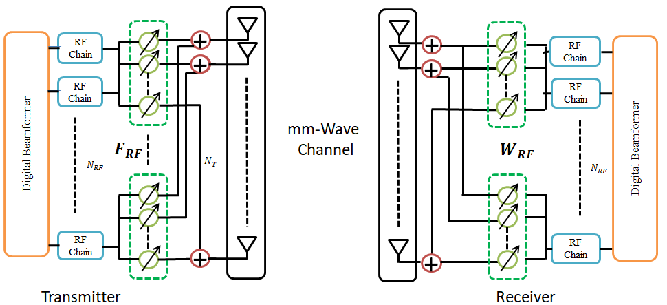
We consider the hybrid beamformer design for a single-user mm-Wave massive MIMO system as shown in Fig. 1. The BS has antennas and RF chains to transmit data streams. In the downlink, the BS first precodes data symbols by applying the baseband precoder . Then the baseband signal is conveyed via an RF precoder to form the transmitted signal . We assume that consists of analog phase shifters, each of which has unit-modulus elements, i.e., . Also, we have the power constraint that is enforced by the normalization of the baseband precoder .
Assuming a block-fading channel model, the received signal at the MS is given by [32]
| (1) |
where represents the average received power, is the mm-Wave channel matrix and is additive white Gaussian noise (AWGN) vector. At the receiver, the received signal is first processed by analog combiners , then the receiver employs low-dimensional digital combiners to process the RF signal to obtain the received symbol vector as , i.e.,
| (2) |
where the analog combiners have element-wise constraint similar to the RF precoders.
II-A Channel Model
In mm-Wave transmission, the channel can be represented by the Saleh-Valenzuela (SV) model where a geometric channel model is adopted with limited scattering [33, 34]. Hence, we assume that the channel matrix includes the contributions of clusters, each of which has scattering paths/rays within the cluster. Thus, we can represent the downlink channel matrix by an matrix as
| (3) |
where denotes the complex gain corresponding to the -th path in the -th cluster, which are assumed to be independent zero-mean Gaussian random variables. and are the and steering vectors representing the array responses of the receive and transmit antenna arrays respectively. In particular, we define the steering vectors of receive and transmit arrays for a uniform linear array (ULA) as and respectively. Here, is the uniform distance between the antennas and is the wavelength for the carrier frequency with the speed of light .
II-B Problem Formulation
We formulate the main problem as designing the hybrid beamformers , by maximizing the overall spectral efficiency of the system. which can be achieved by using the instantaneous channel matrix available at the receiver. We assume that the Gaussian symbols are transmitted through the mm-Wave channel [6, 4, 5], thus, the hybrid beamformer design problem can be stated as follows
| (4) |
where corresponds to the combiner-processed noise term in the received signal (2). and are the feasible sets for the RF precoder and combiners which obey the unit-modulus constraint. In some earlier works [6, 9, 28], and are assumed to be known as the set of array responses of received/transmitted path angles. Then, the hybrid beamformers are designed by maximizing the spectral efficiency through a greedy search over the columns of and . In this paper, we do not have such an assumption. In fact, we design the hybrid beamformers via manifold optimization approach which does not require a predefined codebook as in [6, 9, 28].
In the proposed DL framework without instantaneous CSI feedback (Please see Fig. 2), we make the following assumptions:
Assumption 1: The BS and the MS do not have the knowledge of perfect CSI.
Assumption 2: The BS does not require the CSI, instead it only knows the spatial statistics of the channel, i.e., the covariance of the transmit antenna array at the BS is available through CCM acquisition11 1 We assume that the CCM is available at the BS via CCM estimation approaches such as [35]..
Assumption 3: The MS can estimate the instantaneous channel by processing the received pilot signals transmitted from the BS in the preamble stage.
Assumption 4: We assume that the BS has the trained CovNet which accepts the CCM as input to design the hybrid precoders and . The MS has the trained deep networks ChannelNet and BFNet to estimate the channel and design the hybrid combiners and , respectively.
In the following, we first discuss the channel estimation and hybrid beamforming, then we introduce our DL framework for the considered problem.
III Channel Estimation and CCM Model
In practice, the estimation process of the channel matrix is a challenging task, especially in the case of a large number of antennas taking place in massive MIMO systems [13, 36]. Furthermore, the coherence interval is very small in mm-Wave systems, making the channel estimation and acquisition process more difficult [16]. In a practical scenario, the estimated channel matrix can be obtained by channel estimation techniques [34, 37, 36, 38, 5].
III-A Channel Estimation
In our DL framework, the channel estimation is performed by a deep network using the received pilot signals in the preamble stage. In this case, we assume the downlink scenario where the BS activates only one RF chain to transmit pilot signals on a single beam for . Then, the receiver activates RF chains to apply for to process the received pilots [24, 5, 38]. Since the number of RF chains in the receiver is limited by (), only combining vectors can be used at a single channel use. Hence, the total channel use in the channel acquisition process is . Then, the transmit and receive beamforming matrices become and respectively. Specifically, and can be constructed as the first (or ) column vectors of an (or ) discrete Fourier transform (DFT) matrix [24, 38]. Let us now consider the received signal in (2) in the preamble as
| (5) |
where denotes the pilot signals and is the effective noise matrix where denotes the AWGN matrix which corrupts the pilot training data by SNR. Without loss of generality, we assume , then the received signal in (5) becomes
| (6) |
By processing , we can obtain the initial channel estimate (ICE) as
| (7) |
where and . We call initial channel estimate (ICE) since it will be used further in the proposed DL framework to obtain better channel estimate. Likewise, once is obtained at the receiver, it is fed to the pretrained network ChannelNet to improve the channel estimation performance22 2 ChannelNet is trained by accepting the input as initial channel estimate (ICE), , and maps the input data to the labels which is the true channel matrix . As a result, a better channel estimation performance can be achieved as demonstrated in Section VI.. Then the improved channel estimate is inserted to BFNet to obtain the hybrid combiners.
III-B CCM Model
Statistical beamforming strategies provide infrequent update of the channel information through the channel statistics, but no instantaneous feedback, hence, reducing the feedback overhead [19, 17, 18, 20]. In practice, the CCM can be estimated by several algorithms such as temporal averaging techniques which collect the single snapshot received signals [39], compressed covariance sensing approaches [40] and power angular spectrum estimation [41], etc. Since the CCM acquisition is a certain field of research, in this paper we assume that the CCM is available at the BS, which can be obtained through above algorithms [39, 40, 41, 35]. In this work, we first exploit the structure of the CCM for hybrid precoder design, which will be employed in the proposed DL framework.
Let us consider the channel model in (3) which can be written as
| (8) |
where and and are and steering matrices of paths respectively. is a diagonal matrix which includes the path gains as . Using the property that the channel gains are independent random variables, we can write the covariance of the channel as
| (9) |
where the expectation is performed over . Incorporating the statistics of the AOA/AOD angles and the channel gains, we can rewrite (9) as
| (10) |
Since the receive steering vectors are unit-norm and normalized with , we have . Also, due to the independent zero-mean gains , we also have . Hence, we get
| (11) |
The CCM structure in (11) explicitly implies that instantaneous channel information such as the path gains are not present. Hence, with comparison to the instantaneous channel in (3), the covariance information in (11) does not reflect the same precoding performance due to absence of the instantaneous channel gain information , instead the variance knowledge .
Using only the covariance information in (11), RF precoders and can be designed without requiring the instantaneous CSI feedback. This can be done by the infrequent feedback of , mean AOD angles and the angular spreads [20]. Then, the covariance matrix at the BS can be constructed as
| (12) |
To further reduce the infrequent feedback overhead, these statistical parameters can be quantized and the estimated CCM can be obtained as
| (13) |
where is the set of discrete angles defined as
| (14) |
where is the angular resolution.
IV Hybrid Beamformer Design For mm-Wave MIMO Systems
In this section, we first discuss the design of hybrid beamformers which will be, eventually, the labels of the proposed deep network architecture as discussed in Section V. The design problem of the hybrid beamformers requires a joint optimization as in (II-B), however this approach is computationally prohibitive and even intractable. Instead, a decoupled problem is preferred [6, 11, 29, 12]. Hence, in this work, we first design the hybrid precoders by utilizing the channel covariance matrix . Then, the receiver designs the hybrid combiners where the channel matrix is used.
IV-A Hybrid Analog Precoder Design
In order to design the hybrid precoders, we rewrite the channel covariance matrix in (11) as where . If the angular spread of the received paths is small, then can be approximated as , through eigendecomposition, corresponding to the largest few eigenvalues [20]. denotes the eigenvectors of corresponding to a few eigenvalues of which are placed in descending order in . Then, we can write the approximate form of the channel covariance matrix from (11) as
| (15) |
where and the diagonal elements of are those of . Therefore, the optimum statistical beamformer is the linear combination of the column vectors of , which can also be obtained from the following problem
| (16) |
Once the unconstrained statistical beamformer is obtained, the next task is to determine the analog precoders . One possible solution is to solve
| (17) |
from which we can readily obtain the solution as which takes only the phase information of [20]. However, this approach is sub-optimum. In order to obtain an optimum solution for the RF precoder , we consider the following problem, i.e.,
| (18) |
Above problem can be solved via alternating minimization approach where and are estimated one by one iteratively while one of them is fixed [12, 31]. Although there are closed form expressions to estimate [6], the estimation of is not straightforward due to the element-wise unit modulus constraint, i.e., . Hence, we first discuss the estimation of , by fixing . An effective solution can be achieved via conjugate gradient descent algorithm by using the tools of Riemannian manifolds [42, 12, 31]. Let be the unknown vector to be optimized where , then the search space of (IV-A) can be regarded as a Riemannian submanifold of complex plane since forms a complex circle manifold, i.e., [42]. The Riemannian gradient at , , can be defined as the orthogonal projection of the Euclidean gradient onto the tangent space of , i.e.,
| (19) |
where the Euclidean gradient of the cost function in (IV-A) is given by
| (20) |
Then, the conjugate gradient descent algorithm [42] can be used where the unknown is obtained with the update rule
| (21) |
where is Armijo backtracking line search step size [31] and denotes the direction of decrease defined as
| (22) |
where denotes the Riemannian gradient at the -th iteration and is the Polak-Ribiere parameter [42]. is the vector transport of conjugate direction and it is defined as
| (23) |
where can be directly obtained from (21) and . The optimization process can be initialized from a random point, i.e., where , .
IV-B Hybrid Digital Precoder Design
Once is obtained, the task is to estimate . While the optimum solution for for instantaneous channel information is given in [43, 44], here, we derive the solution by using the statistical channel information, i.e., . Let us rewrite (IV-A) by using as
| (24) |
which maximize the mutual information at the BS, i.e.,
| (25) |
Let us decompose as where and . Denoting , we can write the following optimization problem
| (26) |
Let us define matrix as where . By Hadamard inequality [45], the optimum solution of (IV-B) can be only be achieved if is diagonal. Also from [43, Lemma 12], to form the diagonal matrix , for a given and positive semidefinite Hermitian matrix , it is always possible to find another matrix such that and . Here, the optimum solution, i.e., can be found from the eigenvalue decomposition of as for which we have where denotes the eigenvector matrix corresponding to the eigenvalues in . is water-filling power allocation matrix [43] with
| (27) |
where satisfies . Finally, we can select the optimum solution for as
| (28) |
By updating and from (21) and (28), one can arrive an optimum solution in the sense that (IV-A) is minimized [12, 31].
By designating the optimum solution and from (IV-A) as the labels of the deep network, very good beamforming performance can be obtained [46]. Once the transmitter designs the hybrid precoders via the channel covariance matrix, next we discuss the design of hybrid combiners at the receiver by using the estimated channel matrix obtained from the preamble stage discussed in Section III-A.
IV-C Hybrid Combiner Design
At the receiver, the hybrid combiners are designed by utilizing only the estimated channel matrix from the received pilots. We can write the combiner design problem by minimizing the mean-square-error (MSE) between the transmitted and received-processed symbols as follows
| (29) |
In order to write the problem in (IV-C) in more efficient form, we follow the steps in [6] and add a constant term into the cost function in (IV-C). Here, denotes the MMSE estimator defined as which can be written in a compact form as,
Then, an equivalent problem to (IV-C) can be stated as follows
| (30) |
where denotes the covariance of the receive array output in (1). In (IV-C), the multiplicative term has no element depending on or , therefore, it can be removed since it does not affect the solution. Thus, we can solve the combiner design problem in (IV-C) as
| (31) |
The solution to the optimization problem in (IV-C) is similar to the precoder design problem in (IV-A) and they can be effectively solved via alternating minimization approach by optimizing each unknown term while fixing the another. This can be performed by a MATLAB-based algorithm, called Manopt [31]. Note that (IV-A) and (IV-C) do not require a predefined codebook which includes the set of array responses of the receive and transmit arrays. In fact, the optimization problems can be initialized from a random point, i.e., the beamformers with unit-modulus constraint and random phases.


V Learning-Based Hybrid Beamformer Design
In Fig. 2, we demonstrate the proposed DL framework without instantaneous CSI feedback. We introduce three deep network architectures which are shown in Fig. 3: CovNet, used at the BS only and it learns the channel statistics from and obtain the hybrid precoders and . ChannelNet and BFNet are placed at the MS only, to estimate the channel and construct the hybrid combiners and respectively. In the following, we discuss the details of each deep network architecture.
V-A Designing Input Data For The Deep Networks
In order to enrich the input features, we feed the networks with three ”channel” with notation @ where and denote the 2D sizes of the input. For each ”channel”, we use real, imaginary, absolute value and the phase of each entry of the input data depending on the application. This approach provides good features for fitting the data in the training state as well as extracting new features inherit in the input [28, 29, 30, 24, 47]. In particular, we denote the input for CovNet as whose -th entry of the first, second and the third ”channel” is given by , and , respectively. For ChannelNet, the input is denoted as and, similarly we have , and . Finally, the input for BFNet is given by where , and respectively. We observe, through simulations, that the angular values provide better features and training performance for covariance data whereas the absolute value is more appropriate for and [47]. Hence, the third ”channel” for is selected as the angle information whereas the absolute value is used for the third ”channel” of .
V-B Labeling The Deep Networks
We start by constructing the labels of CovNet which is the hybrid precoders and . Hence, we represent the output label of CovNet by as
| (32) |
which is an real-valued vector. For ChannelNet, we represent the labels by as
| (33) |
which is a real-valued vector of size . Finally, the output label of BFNet is, similar to CovNet, given by as
| (34) |
V-C Network Architectures and Training
The deep networks in Fig. 3, CovNet, ChannelNet and BFNet have the input-output pairs as , and respectively. For each network, we use three convolutional layers with kernel size of . While CovNet has 256 convolutional filters, ChannelNet and BFNet have 128 filters. In addition, CovNet and BFNet have two pooling layers, which reduce the dimension by two, after the first two convolutional layers whereas ChannelNet has no pooling layer. There are two fully connected layers in CovNet and BFNet and three fully connected layers are placed in ChannelNet. There are dropout layers with a probability after each fully connected layer in each network. The output layer of all networks are the regression layer with proper size depending on the application as discussed in Section V-B. While the other network architectures with different parameters are also possible, the presented network parameters are one possible solution to obtain good performance for the considered problem. We have obtained the network parameters from a hyperparameter tuning process providing the best performance for the considered scenario [28, 29, 47, 30, 24].
The proposed deep networks are realized and trained in MATLAB on a PC with a single GPU and a 768-core processor. We have summarized the algorithmic steps for training data generation in Algorithm 2. We have used the stochastic gradient descent algorithm with momentum 0.9 and updated the network parameters with learning rate and mini-batch size of samples. Then, we have reduced the learning rate by the factor of after each 20 epochs. We also applied a stopping criteria during training such that the training terminates if the validation accuracy does not improve in three consecutive epochs. To train the proposed CNN structures, different scenarios are realized for as in Algorithm 2. For each scenario, we generated a channel matrix (together with the corresponding covariance matrix) and received pilot signal where synthetic additive noise is added to the training data on the CCM, channel matrix and the received pilot signal which are defined by SNRR, SNRH and SNR respectively33 3 In the simulations, we have used four SNR definitions, all of which are characterized by AWGN. 1) SNR, SNR: SNR on the signal in (6) when the pilot signals are received in the preamble for training and test stage respectively. 2) SNRH: SNR on the channel matrix to obtain the corrupted channel data in training. 3) SNRR : SNR on the channel covariance matrix to obtain the corrupted channel covariance data in training. 4) Finally, we use the term ”SNR” on the received signal in (1) (not in the preamble) for hybrid beamforming process.. In the training process we use multiple SNRR, SNRH and SNR values to make the networks robust against corrupted input characteristics [28, 29]. Hence we use SNR dB, SNR dB and SNR dB. Hence, we define SNR, SNR and SNR where are the variance of AWGN corresponding to the input data. As a result, 180000 input-output pairs are generated for training. In the training process, and of all generated data are selected as the training and validation datasets, respectively. For the prediction process, we have generated a test data which is separately generated by adding noise on received pilot signal with SNR. Note that this allows us to further corrupt the input data and test the network against deviations in the input data which can resemble the changes in the mm-Wave channel [16].
V-D Online Deployment of the Proposed DL Approach
The adaptation of the DL network to the changes in the propagation environment is very important since the offline training cannot include all possible channel characteristics. In this part, we investigate the online performance of the proposed DL approach for channel estimation. In particular, ChannelNet is trained offline as described in Algorithm 2. Then, it is deployed online where the instantaneous channel parameters such as , and change due to the motion of MS. Let be the received pilot signal at time , which is constructed as in the -th steps of Algorithm 2. Since in the online stage the channel matrix is unknown, is used to estimate the channel by both ChannelNet and also an analytical channel estimation technique such as angle domain channel estimation (ADCE) approach proposed in [38], which has close-to-CRB (Cramer-Rao lower bound) performance. Then, the DL network is updated if its performance is poor, otherwise it continues with its current form. Let us define the error metric at time as which is defined as
| (35) |
where is the last estimated channel matrix via ADCE. Note that the channel estimation via ADCE is only performed at the beginning of the online deployment and when the network is updated. By doing so, the channel estimation complexity is reduced thanks to the low computation time of DL network. The network updates its parameters if
| (36) |
holds for some threshold parameter which determines how frequently the network is updated. If , then it means that ChannelNet performs satisfactorily and it continues to work without update. Let us denote network parameters at time as , then, we update only the higher layers (i.e., the fully connected layers) of , which are more environment-dependent. The lower layers (i.e., convolutional layers) are kept intact or frozen because they generally behave like problem-dependent [48]. In Algorithm 2, we describe the steps for online deployment. Here SNR is used to introduce noisy inputs for to provide robustness.
During online deployment, the complexity of the training is low due to the small size of dataset. Furthermore, the online training is only performed if the propagation environment changes significantly. Hence, the proposed DL approach does not need to be re-trained for each time instance, which lowers the computational complexity.
V-E Computational Complexity and Power Consumption
The computational complexity of the proposed DL approach has two main parts, namely, online prediction and offline training. While the online complexity has simple expressions, the complexity analysis of the offline training is still an open issue due to the complex implementation of backpropagation process involved during training. Therefore, we only consider the complexity of online prediction stage.
For a deep neural network with convolutional layers and fully connected layers [49], the total time complexity of convolutional layers is where are the convolutional kernel size, are the 2D output size of the -th convolutional layer and is the number of filters of the -th layer. The total complexity of the fully connected layers is where is the number of units in the fully connected layer. The comparison of computational complexity for a DL network with a conventional analytical method is not fair due to the use of different processing units, i.e., DL benefits the use of GPU, while not all analytical method are implementable via GPU [49]. For this reason, we compare the computation times of both algorithms in the simulations section.
Next, we compare the power consumption of the conventional systems and the DL-based methods. For a conventional mm-Wave system with transmit power W, total power consumption can be given as
| (37) |
where , and are the power consumption of an RF chain, phase shifter and baseband processing respectively. Furthermore, they are given approximately as mW, mW and mW, for which becomes approximately W for and [34]. While there is no commercial DL-based hardware for mm-Wave system configuration, there exist some processing units that can run DL methods effectively such as Intel Movidius [50] which has power consumption of approximately mW [51, 50]. This shows that DL-based methods can be a promising candidate for next generation wireless communication systems providing reasonable performance and lower computation complexity.
VI Numerical Simulations
In this section, we have evaluated the performance of the proposed approach (called SDHB: statistical deep hybrid beamforming) through several experiments. We compare the proposed approach with both statistical and non-statistical hybrid beamforming techniques such as SHB [20] (which solves (IV-A)), PE-HB [11] and deep learning-based hybrid beamforming (DLHB) [28] as well as the MO algorithm [12]. Note that the performance of the MO algorithm constitutes an upper bound for DLHB/SDHB since the network labels of DLHB/SDHB are obtained by MO. Therefore, DLHB/SDHB cannot perform better than MO. We further evaluate the performance of the fully digital beamforming performance as a benchmark. In order to compare the channel estimation performance of ChannelNet, we implement the SF-CNN algorithm [24] with the same network parameters and feed with the same input, i.e., the initial channel estimates.
Throughout the simulations, we consider a single-user massive MIMO system with RF chains for and antennas. The antennas are deployed with half wavelength spacing at GHz. We assume, unless stated otherwise, there are clusters of all transmit and receive paths which are uniform randomly selected from the interval with angular spread of . In preamble stage, the transmitter emits only one beam by using a single RF chain while, at the receiver, all of the RF chains are active. The transmit and received beams are formed by selecting and as and DFT matrices respectively [24].

In Fig. 4, we present the spectral efficiency with respect to SNR when SNR dB. As expected, we see that the non-statistical approaches (MO, PE-HB, DLHB) perform superior than the statistical approaches (SHB, SDHB) including the fully-digital beamforming performance, thanks to the available instantaneous CSI knowledge. In statistical approaches, the CCM does not fully reflect the instantaneous channel data which changes in time due to the parameters such as the channel gain . We can also see that DL-based approaches outperform the non-DL techniques such as PE-HB and SHB. In particular, the proposed approach SDHB closely follows the fully-digital beamforming for statistical case. The outperformance of SDHB can be attributed to the use of optimum hybrid beamformers as labels, which are obtained by the MO algorithm [12] whereas SHB simply takes the phases of which is sub-optimum. Furthermore, as will be demonstrated later, the time complexity of the proposed DL-based approach is much lower as compared to the MO, thus making it a very efficient algorithm.
In Fig. 5, the robustness of the algorithms is investigated with respect to the estimated channel data. Hence, for all of the beamforming algorithms, we use the channel matrix estimated by ChannelNet when the received pilot data is corrupted by noise determined by SNR. Note that the noise introduced by SNR only affects the combiner design (not the precoder design) performance of the statistical approaches (SHB and SDHB) since they only use estimated channel data in the combiner design stage. We can see from Fig. 5 that all of the algorithms reach their maximum performance after SNR dB. In particular, SDHB has more robust performance than SHB and performs very close to the fully-digital beamformer. This observation states that the algorithms require at least approximately SNR dB noise level for sufficient channel estimate in this setting.
For the same experiment, we also examine the channel estimation performance in terms of normalized MSE in Fig. 6. We see that both ChannelNet and SF-CNN outperform the initial channel estimate obtained from the received pilots. We also see that ChannelNet outperforms SF-CNN which cannot do well, especially for high SNR. The poor performance of SF-CNN is because SF-CNN uses several convolutional layers and no fully connected layer. While convolutional layers are good at extracting new features from the input, fully connected layers are more powerful in terms of mapping the input data to the output [49].


Thanks to the three fully connected layers in ChannelNet, it achieves much less NMSE than SF-CNN. Another disadvantage of SF-CNN [24] is that SF-CNN works properly in the prediction stage only if the SNR in the prediction stage is the same as of the training stage, i.e., SNR = SNR is required. Such a requirement is not needed in our DL framework thanks to the use of multiple SNR levels during training. We see that the performance of both ChannelNet and SF-CNN makes out as SNR increases, especially for SNR dB. This is due to the lack of precision of the deep networks, which are biased estimators in nature. Higher precision can still be obtained if larger number of units in the network layers are used with less training data size. However, this will cause the network memorize the input data so that the network will not function if input data differs from the ones used in the training data set [47]. This fact suggests that the training data should not include too much indistinguishable (noisy) data to provide good precision.


In Fig 7, we present the performance of the algorithms when there is an angular mismatch in the received path angles between the channel matrix used in the training data and the test data. Specifically, the trained networks are fed with the channel data that is generated by introducing angular mismatch in the AOA/AOD angles of all received paths of the channel matrices used in the training data. In a similar way, we also introduce angular mismatch in the CCM data that is used for CovNet and SHB. We observe from Fig. 7 that as the standard deviation of the angular mismatch increases, expectedly, the spectral efficiency performance becomes poorer due to the loss in the channel estimation performance. We see that DL-based approaches provide more robust performance and become resilient up to approximately 4 degrees angular mismatch between training and test data. We note here that more robustness may still be achieved if the training data will be enriched by adding more channel realizations with different angular information. The trade-off here is that if the number of channel realizations is high, the ability of the network to distinguish different input characteristics will be reduced due to the fact that mismatched channel matrices will become more similar, thus the network will yield the same, or least very similar, hybrid beamformer weights at the output. In our simulations, we have used , channel realizations and add synthetic noise into those realizations to make the network more robust against mismatched data. Since the main cause of the performance loss in Fig. 7 is the channel estimation accuracy, we further investigate the channel estimation NMSE with respect to the angular mismatch in Fig. 8. As it is seen, the angular mismatch deteriorates the channel estimation performance. These results support the robustness of the DL-based approaches obtained in Fig. 7.

| Fully-Digital | Fully-Digital, Stat. | MO [12] | DLBH [28] | CovNet | ChannelNet | BFNet | SF-CNN [24] | PE-HB [11] | SHB [20] | |
|---|---|---|---|---|---|---|---|---|---|---|
| 4 | 0.0054 | 0.0501 | 0.6621 | 0.0110 | 0.0143 | 0.0054 | 0.0064 | 0.0054 | 0.0312 | 0.0218 |
| 8 | 0.0057 | 0.0535 | 0.7247 | 0.0117 | 0.0145 | 0.0061 | 0.0073 | 0.0072 | 0.0358 | 0.0292 |
| 16 | 0.0060 | 0.0565 | 1.6754 | 0.0119 | 0.0166 | 0.0073 | 0.0087 | 0.0081 | 0.0426 | 0.0424 |
| 32 | 0.0064 | 0.0574 | 1.6108 | 0.0136 | 0.0184 | 0.0091 | 0.0101 | 0.0094 | 0.0535 | 0.0475 |
| 64 | 0.0079 | 0.0589 | 2.5603 | 0.0147 | 0.0211 | 0.0108 | 0.0108 | 0.0103 | 0.0637 | 0.0481 |
| 128 | 0.0083 | 0.0612 | 4.4153 | 0.0165 | 0.0232 | 0.0118 | 0.0124 | 0.0123 | 0.0763 | 0.0590 |
Fig. 9 illustrates the system rate performance of the algorithms with respect to the number of clusters when . We see that the system rate increases when the spatial diversity of the channel is low (e.g., ). When the diversity is high and the channel becomes less sparse, the performance of the algorithms deteriorates after since the eigenvectors of with respect to dominant eigenvalues do not represent the array response of the received clusters. We also observe that the increase in the number of clusters affects statistical approaches more significantly as compared to the non-statistical approaches. We have used, in this experiment, three values such as when generating the training data so that robust performance can be obtained. Hence, the total length of the training dataset three times greater than the one given in Section V-C. It can be seen from Fig. 9 that SDHB has robust performance against different number of clusters even when .

We further investigate the computation time of the algorithms illustrated in Table I for different number of BS antennas while the other parameters are fixed. We first compare the computation time of statistical and non-statistical fully-digital beamforming. We can see that statistical approach takes longer due to eigendecomposition of the CCM. Among all, the MO algorithm requires the longest time due to the involvement of the optimization stage. For a fair comparison, we can compare the computation time of CovNet and BFNet combined, with the other algorithms such as MO, DLHB, PE-HB and SHB which do not involve channel estimation state. We can see that the proposed DL framework is the fastest algorithm among the all. Combining the complexity of all proposed deep networks CovNet, ChannelNet and BFNet, we obtain approximately the same complexity with comparison to SHB which assumes perfect CSI. In contrast, compared to the MO algorithm, the proposed DL approach is at least 10 times faster (when , and 80 times faster if ), which shows the potential of the proposed DL approach.
Above complexity analysis is valid with the assumption that the proposed DL model is trained beforehand. Therefore, we also discuss the offline training complexity. The convergence of the proposed neural network architecture takes about hours with the aforementioned training dataset and network settings. While this time duration is much larger than the computation time of the trained network, it is only performed once in the offline stage.
Next, we examine the online prediction performance of ChannelNet, as illustrated in Fig. 10. In this experiment, the DL network is deployed online when there is angle mismatch between the AOD/AOA angles of the training and the test data. Then we model the user motion such that changes from to . We select , and use ADCE [38] algorithm to obtain the online labels as described in Algorithm 2. We can see that the performance of the offline network gets poorer as increases since its performance degrades due to the mismatch of the new incoming data. For the online deployment case, the network is updated when the update rule triggers so that the network adapts the environment and its performance gets better when updated. It is shown that network requires to be re-trained for approximately every mismatch, similar to the observations in Fig. 7. To account for the time complexity, the online update (i.e., training with the online dataset) of the network only takes about s while offline training overhead is about hours. This is mainly because of the use of small online dataset. Nevertheless, such small dataset provides very good NMSE performance. In addition, the computation time for employing the network for channel estimation is similar to the results given in Table I. As a result, the online training not only improves the estimation performance, but also accelerates the network training to adapt to the new environment.
VII Summary
We introduced a DL framework for hybrid beamforming and channel estimation for mm-Wave massive MIMO systems without instantaneous CSI feedback. We designed three CNNs, one of which, CovNet is used at the BS to design the precoders by using the channel covariance matrix. Two CNNs, ChannelNet and BFNet are placed at the receiver for channel estimation and combiner design, respectively. We have examined the online deployment of the proposed DL-based channel estimation scheme and shown that the proposed approach can adapt itself to the propagation environment and update its parameters accordingly. We have also shown that the proposed scheme can work properly up to degrees angular mismatch and do not need to be retrained. In another challenging experiment where we present the performance against the number of clusters, we have shown that the proposed approach has robust performance even when the number of clusters differs in the training and the test data. In addition, we have shown that the proposed approach can perform at least times faster than the optimization based approaches in online deployment. It is also worthwhile to mention that the offline training takes much longer than online computation time, however this process is only performed once. Moreover, the proposed online training scheme reduces the training overhead significantly without the requirement of re-training the DL model from scratch.
References
- [1] R. W. Heath, N. González-Prelcic, S. Rangan, W. Roh, and A. M. Sayeed, “An overview of signal processing techniques for millimeter wave MIMO systems,” IEEE J. Sel. Topics Signal Process., vol. 10, no. 3, pp. 436–453, 2016.
- [2] J. G. Andrews, S. Buzzi, W. Choi, S. V. Hanly, A. Lozano, A. C. K. Soong, and J. C. Zhang, “What will 5G be?” IEEE J. Sel. Areas Commun., vol. 32, no. 6, pp. 1065–1082, 2014.
- [3] J. A. Hodge, K. V. Mishra, and A. I. Zaghloul, “Reconfigurable metasurfaces for index modulation in 5G wireless communications,” in IEEE Int. Appl. Comput. Electromagn. Soc. Symp., 2019, pp. 1–2.
- [4] A. Alkhateeb, O. E. Ayach, G. Leus, and R. W. Heath, “Hybrid precoding for millimeter wave cellular systems with partial channel knowledge,” in IEEE Inf. Th. Appl. Workshop, 2013, pp. 1–5.
- [5] ——, “Channel Estimation and Hybrid Precoding for Millimeter Wave Cellular Systems,” IEEE J. Sel. Topics Signal Process., vol. 8, no. 5, pp. 831–846, 2014.
- [6] O. E. Ayach, S. Rajagopal, S. Abu-Surra, Z. Pi, and R. W. Heath, “Spatially sparse precoding in millimeter wave MIMO systems,” IEEE Trans. Wireless Commun., vol. 13, no. 3, pp. 1499–1513, 2014.
- [7] F. Rusek, D. Persson, B. K. Lau, E. G. Larsson, T. L. Marzetta, O. Edfors, and F. Tufvesson, “Scaling up MIMO: Opportunities and challenges with very large arrays,” IEEE Signal Process. Mag., vol. 30, no. 1, pp. 40–60, 2013.
- [8] L. Wei, R. Q. Hu, Y. Qian, and G. Wu, “Key elements to enable millimeter wave communications for 5G wireless systems,” IEEE Wireless Commun., vol. 21, no. 6, pp. 136–143, December 2014.
- [9] A. Alkhateeb, G. Leus, and R. W. Heath, “Limited feedback hybrid precoding for multi-user millimeter wave systems,” IEEE Trans. Wireless Commun., vol. 14, no. 11, pp. 6481–6494, 2015.
- [10] Z. Wang, M. Li, Q. Liu, and A. L. Swindlehurst, “Hybrid Precoder and Combiner Design With Low-Resolution Phase Shifters in mmWave MIMO Systems,” IEEE J. Sel. Topics Signal Process., vol. 12, no. 2, pp. 256–269, May 2018.
- [11] F. Sohrabi and W. Yu, “Hybrid analog and digital beamforming for mmWave OFDM large-scale antenna arrays,” IEEE J. Sel. Areas Commun., vol. 35, no. 7, pp. 1432–1443, 2017.
- [12] X. Yu, J. Shen, J. Zhang, and K. B. Letaief, “Alternating Minimization Algorithms for Hybrid Precoding in Millimeter Wave MIMO Systems,” IEEE J. Sel. Topics Signal Process., vol. 10, no. 3, pp. 485–500, April 2016.
- [13] Z. Marzi, D. Ramasamy, and U. Madhow, “Compressive Channel Estimation and Tracking for Large Arrays in mm-Wave Picocells,” IEEE J. Sel. Topics Signal Process., vol. 10, no. 3, pp. 514–527, April 2016.
- [14] H. Yin, D. Gesbert, M. Filippou, and Y. Liu, “A Coordinated Approach to Channel Estimation in Large-Scale Multiple-Antenna Systems,” IEEE J. Sel. Areas Commun., vol. 31, no. 2, pp. 264–273, February 2013.
- [15] A. Li and C. Masouros, “Hybrid Analog-Digital Millimeter-Wave MU-MIMO Transmission With Virtual Path Selection,” IEEE Commun. Lett., vol. 21, no. 2, pp. 438–441, 2017.
- [16] E. Björnson, L. Van der Perre, S. Buzzi, and E. G. Larsson, “Massive MIMO in sub-6 GHz and mmWave: Physical, practical, and use-case differences,” IEEE Trans. Wireless Commun., vol. 26, no. 2, pp. 100–108, 2019.
- [17] T. Liu, J.-K. Zhang, and K. M. Wong, “Optimal precoder design for correlated mimo communication systems using zero-forcing decision feedback equalization,” IEEE Trans. Signal Process., vol. 57, no. 9, pp. 3600–3612, 2009.
- [18] S. A. Jafar and A. Goldsmith, “Transmitter optimization and optimality of beamforming for multiple antenna systems,” IEEE Trans. Wireless Commun., vol. 3, no. 4, pp. 1165–1175, 2004.
- [19] S. Park, J. Park, A. Yazdan, and R. W. Heath, “Exploiting spatial channel covariance for hybrid precoding in massive MIMO systems,” IEEE Trans. Signal Process., vol. 65, no. 14, pp. 3818–3832, 2017.
- [20] Y. Lin, “Hybrid MIMO-OFDM beamforming for wideband mmWave channels without instantaneous feedback,” IEEE Trans. Signal Process., vol. 66, no. 19, pp. 5142–5151, 2018.
- [21] H. Huang, J. Yang, H. Huang, Y. Song, and G. Gui, “Deep learning for super-resolution channel estimation and doa estimation based massive mimo system,” IEEE Trans. Veh. Technol., vol. 67, no. 9, pp. 8549–8560, Sept 2018.
- [22] A. Liao and Z. Gao, “Super-Resolution Channel Estimation for mmWave Massive MIMO,” in 2018 IEEE International Conference on Communications (ICC), 2018, pp. 1–5.
- [23] H. Ye, G. Y. Li, and B. Juang, “Power of deep learning for channel estimation and signal detection in OFDM systems,” IEEE Wireless Commun.ications Lett.ers, vol. 7, no. 1, pp. 114–117, 2018.
- [24] P. Dong, H. Zhang, G. Y. Li, I. S. Gaspar, and N. NaderiAlizadeh, “Deep CNN-Based Channel Estimation for mmWave Massive MIMO Systems,” IEEE J. Sel. Areas Commun., vol. 13, no. 5, pp. 989–1000, Sep. 2019.
- [25] C. Wen, W. Shih, and S. Jin, “Deep Learning for Massive MIMO CSI Feedback,” IEEE Wireless Commun. Lett., vol. 7, no. 5, pp. 748–751, Oct 2018.
- [26] H. Huang, Y. Song, J. Yang, G. Gui, and F. Adachi, “Deep-learning-based millimeter-wave massive MIMO for hybrid precoding,” IEEE Trans. Veh. Technol., vol. 68, no. 3, pp. 3027–3032, 2019.
- [27] A. Alkhateeb, S. Alex, P. Varkey, Y. Li, Q. Qu, and D. Tujkovic, “Deep learning coordinated beamforming for highly-mobile millimeter wave systems,” IEEE Access, vol. 6, pp. 37 328–37 348, 2018.
- [28] A. M. Elbir, “CNN-based precoder and combiner design in mmWave MIMO systems,” IEEE Commun. Lett., vol. 23, no. 7, pp. 1240–1243, 2019.
- [29] A. M. Elbir and K. V. Mishra, “Joint Antenna Selection and Hybrid Beamformer Design using Unquantized and Quantized Deep Learning Networks,” IEEE Trans. Wireless Commun., 2019, in press.
- [30] A. M. Elbir and A. Papazafeiropoulos, “Hybrid Precoding for Multi-User Millimeter Wave Massive MIMO Systems: A Deep Learning Approach,” IEEE Trans. Veh. Technol., pp. 1–1, 2019.
- [31] N. Boumal, B. Mishra, P.-A. Absil, and R. Sepulchre, “Manopt, a Matlab Toolbox for Optimization on Manifolds,” Journal of Machine Learning Research, vol. 15, pp. 1455–1459, 2014. [Online]. Available: http://jmlr.org/papers/v15/boumal14a.html
- [32] E. Torkildson, C. Sheldon, U. Madhow, and M. Rodwell, “Millimeter-Wave Spatial Multiplexing in an Indoor Environment,” in 2009 IEEE Globecom Workshops, Nov 2009, pp. 1–6.
- [33] R. Méndez-Rial, C. Rusu, A. Alkhateeb, N. González-Prelcic, and R. W. Heath, “Channel estimation and hybrid combining for mmWave: Phase shifters or switches?” in IEEE Information Theory and Applications Workshop, 2015, pp. 90–97.
- [34] R. Méndez-Rial, C. Rusu, N. González-Prelcic, A. Alkhateeb, and R. W. Heath, “Hybrid MIMO architectures for millimeter wave communications: Phase shifters or switches?” IEEE Access, vol. 4, pp. 247–267, 2016.
- [35] A. O. Kalayci and G. M. Guvensen, “An Efficient Beam and Channel Acquisition via Sparsity Map and Joint Angle-Delay Power Profile Estimation for Wideband Massive MIMO Systems,” arXiv preprint arXiv:1910.05815, 2019.
- [36] J. Wang, Z. Lan, C. woo Pyo, T. Baykas, C. sean Sum, M. A. Rahman, J. Gao, R. Funada, F. Kojima, H. Harada, and S. Kato, “Beam codebook based beamforming protocol for multi-Gbps millimeter-wave WPAN systems,” IEEE J. Sel. Areas Commun., vol. 27, no. 8, pp. 1390–1399, October 2009.
- [37] W. U. Bajwa, J. Haupt, G. Raz, and R. Nowak, “Compressed channel sensing,” in Annual Conference on Information Sciences and Systems, March 2008, pp. 5–10.
- [38] D. Fan, F. Gao, Y. Liu, Y. Deng, G. Wang, Z. Zhong, and A. Nallanathan, “Angle Domain Channel Estimation in Hybrid Millimeter Wave Massive MIMO Systems,” IEEE Trans. Wireless Commun., vol. 17, no. 12, pp. 8165–8179, Dec 2018.
- [39] I. S. Reed, J. D. Mallett, and L. E. Brennan, “Rapid Convergence Rate in Adaptive Arrays,” IEEE Trans. Aerosp. Electron. Syst., vol. AES-10, no. 6, pp. 853–863, Nov 1974.
- [40] D. Romero, D. D. Ariananda, Z. Tian, and G. Leus, “Compressive Covariance Sensing: Structure-based compressive sensing beyond sparsity,” IEEE Signal Process. Mag., vol. 33, no. 1, pp. 78–93, Jan 2016.
- [41] H. Xie, F. Gao, S. Jin, J. Fang, and Y. Liang, “Channel estimation for tdd/fdd massive mimo systems with channel covariance computing,” IEEE Trans. Wireless Commun., vol. 17, no. 6, pp. 4206–4218, June 2018.
- [42] P.-A. Absil, R. Mahony, and R. Sepulchre, Optimization Algorithms on Matrix Manifolds. Princeton, NJ, USA: Princeton University Press, 2007.
- [43] D. P. Palomar, J. M. Cioffi, and M. A. Lagunas, “Joint Tx-Rx beamforming design for multicarrier MIMO channels: a unified framework for convex optimization,” vol. 51, no. 9, pp. 2381–2401, 2003.
- [44] A. Alkhateeb and R. W. Heath, “Frequency selective hybrid precoding for limited feedback millimeter wave systems,” IEEE Trans. Commun., vol. 64, no. 5, pp. 1801–1818, 2016.
- [45] M. Z. Shakir, T. S. Durrani, and M.-S. Alouini, “Hadamard upper bound on optimum joint decoding capacity of wyner gaussian cellular mac,” EURASIP Journal on Wireless Communications and Networking, vol. 2011, no. 1, p. 110, 2011.
- [46] A. M. Elbir and K. V. Mishra, “Low-complexity limited-feedback deep hybrid beamforming for broadband massive mimo communications,” arXiv preprint arXiv:1910.14240, 2019.
- [47] A. M. Elbir, K. V. Mishra, and Y. C. Eldar, “Cognitive radar antenna selection via deep learning,” IET Radar, Sonar & Navigation, vol. 13, pp. 871–880, 2019.
- [48] S. J. Pan, I. W. Tsang, J. T. Kwok, and Q. Yang, “Domain adaptation via transfer component analysis,” IEEE Transactions on Neural Networks, vol. 22, no. 2, pp. 199–210, 2010.
- [49] K. Simonyan and A. Zisserman, “Very deep convolutional networks for large-scale image recognition,” CoRR, vol. abs/1409.1556, 2015.
- [50] B. Barry, C. Brick, F. Connor, D. Donohoe, D. Moloney, R. Richmond, M. O’Riordan, and V. Toma, “Always-on vision processing unit for mobile applications,” IEEE Micro, vol. 35, no. 2, pp. 56–66, 2015.
- [51] M. Murshed, C. Murphy, D. Hou, N. Khan, G. Ananthanarayanan, and F. Hussain, “Machine learning at the network edge: A survey,” arXiv preprint arXiv:1908.00080, 2019.
![[Uncaptioned image]](2006.10971v2/a4_2.jpg) |
Ahmet M. Elbir (Senior Member, IEEE) received the B.S. degree (with Hons.) in electrical engineering from Firat University in 2009, and the Ph.D. degree in electrical engineering from Middle East Technical University (METU) in 2016. He is currently a Visiting Postdoctoral Researcher with Koc University, and a Research Fellow with Duzce University. His research interests include array signal processing, sparsity-driven convex optimization, signal processing for communications, and deep learning for array signal processing. He was a recipient of the 2016 METU Best Ph.D. Thesis Award for his Doctoral Studies. He has been serving as an Associate Editor for IEEE ACCESS and Frontiers in Communications and Networks. |