Predictive Complexity Priors
Eric Nalisnick Jonathan Gordon José Miguel Hernández-Lobato
University of Amsterdam University of Cambridge University of Cambridge
Abstract
Specifying a Bayesian prior is notoriously difficult for complex models such as neural networks. Reasoning about parameters is made challenging by the high-dimensionality and over-parameterization of the space. Priors that seem benign and uninformative can have unintuitive and detrimental effects on a model’s predictions. For this reason, we propose predictive complexity priors: a functional prior that is defined by comparing the model’s predictions to those of a reference model. Although originally defined on the model outputs, we transfer the prior to the model parameters via a change of variables. The traditional Bayesian workflow can then proceed as usual. We apply our predictive complexity prior to high-dimensional regression, reasoning over neural network depth, and sharing of statistical strength for few-shot learning.
1 INTRODUCTION
Choosing the prior for a Bayesian model is the most important—and often, the most difficult—step in model specification (Robert 2001). Unfortunately, prior specification within machine learning is additionally fraught and challenging. Popular models such as neural networks (NNs) are high dimensional and unidentifiable, making it extremely hard to reason about what makes a good prior. Moreover, since the true posterior can almost never be recovered, it is difficult to isolate a prior’s influence (even empirically). We are left asking: do the specifics of the prior even matter if they are blunted by our posterior approximations and large data sets? Until recently, most work in machine learning has assumed the negative and resorted to priors of convenience. For instance, the standard normal distribution is by far the most popular prior for Bayesian NNs (Zhang et al. 2020; Heek and Kalchbrenner 2019; Wenzel et al. 2020).
In this paper, we present a novel framework to specify priors for black-box models. Rather than working with the uninterpretable parameter space, we place the Bayesian prior on the model’s functional complexity. Our prior, termed the predictive complexity prior (PredCP), compares the model’s predictions to those of a reference model. For example, we define the reference model for a NN to be a NN with one fewer layer. The PredCP can then assess and control the effect of depth on the model’s capacity. Unlike previous work on functional priors (Sun et al. 2019), we use a change of variables to exactly translate the functional prior into a proper prior on the model parameters. Bayesian inference can then proceed as usual and without involving extra machinery. We claim the following contributions:
- •
Methodology: We propose predictive complexity priors (PredCPs). These extend Simpson et al. 2017’s framework to the model predictions, thereby allowing our data-space intuitions to guide prior specification. Moreover, we introduce crucial modifications that allow the PredCP to scale to large, black-box models such as NNs.
- •
Applications: We demonstrate the wide applicability of the PredCP by using it for three disparate tasks: high-dimensional regression, reasoning over depth in Bayesian NNs, and sharing information across tasks for few-shot learning. For Bayesian NNs, we investigate the PredCP’s behavior in detail, revealing its mechanism of action: regularizing predictive variance.
- •
Experiments: We report results across a variety of tasks (classification, regression, few-shot learning), models (logistic regression, NNs), and posterior inference strategies (Markov chain Monte Carlo, variational inference, MAP estimation). The PredCP provides consistent improvements in predictive generalization over alternative priors (uninformative, shrinkage).
2 SETTING OF INTEREST
Notation
Matrices are denoted with upper-case and bold letters (e.g. ), vectors with lower-case and bold (e.g. ), and scalars with no bolding (e.g. or ). We use italics to differentiate observations and constants (e.g. , ) from random variables (e.g. , ).
Model
We consider hierarchical models of the form:
| (1) |
where is the data (sampling) model, is a first-level prior, and is a second-level hyper-prior. We are primarily concerned with models for which is parameterized by a complicated function and plays a significant role in controlling the complexity of that function. One such example is parameterizing with a NN whose weights are given a normal prior with variance : . As grows, the weights become less constrained and the model becomes more flexible. A common strategy for controlling is to give it a shrinkage prior such as a zero-favoring inverse gamma (Neal 1994) or half-Cauchy (Carvalho et al. 2009). While this is a sensible approach, it can be hard to understand how regularizes the downstream predictive function (Piironen and Vehtari 2017b).
A Sketch of Our Approach
We propose a novel prior for that goes beyond simply encouraging its value to be small, as a shrinkage prior does. Instead, we control via model-based (Gelman et al. 2017) functional regularization. Inspired by Simpson et al. 2017,11 1 We provide a detailed summary of and comparison to Simpson et al. 2017’s framework in Section 6 we define a divergence function between the model of interest—denote it for now—and a reference model denoted , which does not depend on . Denote the divergence as . We derive by placing a prior on and reparameterizing w.r.t. : , where denotes the inverse of the aforementioned divergence function. The -prior’s density function can then be written using the change of variables formula:
| (2) |
where is the absolute value of the divergence function’s derivative w.r.t. . Note that must be differentiable and bijective for to be proper (i.e. integrate to one).22 2 We discuss bijectivity conditions for NNs in Section 5. For these conditions to be satisfied, must be a scalar since is a scalar.
These technical conditions aside, the crucial property of our framework is that the divergence is computed by integrating over , the random variable that corresponds to data. In turn, the prior can represent data-space intuitions (via ) and automatically translate them (via ) into a prior on the model parameters. This direction runs counter to how priors are usually defined: by specifying directly and having little-to-no information about the induced distribution on . Despite its dependence on the observation model, we emphasize that our prior is not an empirical Bayesian prior (Casella 1985) since is integrated out.
3 IDEALIZED SETTING
In order to implement the prior sketched in Equation 2, we need to make both theoretical choices (e.g. the divergence) and practical choices. We separate the description of our prior into two sections (3 and 4) so as to delineate theory from practice. In this section, we provide a full theoretical description. Section 4 then introduces some modifications that increase the scalability and broaden the applicability of our prior.


We call the idealized version the evidence complexity prior (ECP). It implements Equation 2 via the following three steps:
Step #1: Define Reference Model
Given the model of interest in Equation 1, the first step is defining the reference model . Crucially, denotes a random variable that corresponds to data, not an observation. Thus, we call and ‘evidence functions’ (Bishop 2006), not marginal likelihoods. In general, we define by replacing the first-level prior with a less expressive prior . We obtain the final version of the reference model by marginalizing over :
| (3) |
We will exclusively use a point-mass prior so that this integration is made trivial: . To form a corresponding representation of our model of interest, we marginalize over :
| (4) |
For many models, it will be hard to perform the above integration, which is why we refer to the ECP’s construction as ‘idealized.’
Step #2: Define Divergence
We next choose the divergence function. Following Simpson et al. 2017, we use the Kullback–Leibler divergence (KLD):
| (5) |
We choose this particular KLD—using as the first argument—because it represents the bits lost when we approximate with the reference model. Switching the arguments would not be sensible since quantifies the bits lost when approximates , which should be easy to do since is more expressive. Other choices of divergence (e.g. Hellinger) are possible, but in Section 4, we will require that the divergence be a convex function w.r.t. .
Step #3: Reparameterize
Lastly, we place a prior on the divergence: . The support of should be to match the KLD’s codomain.33 3 If ’s support is , then we assume a small constant is added to the KLD so that it never evaluates to zero. The degree to which favors represents our preference for the simpler reference model. As allocates more density away from zero, the functional regularization is relaxed. Performing the change of variables then yields the ECP on :
| (6) |
The crucial characteristics of the ECP are that it compares the models holistically and in data space. Using the evidence functions (step #1) allows the ECP to directly assess how affects . Hence the ECP embraces the philosophy that the prior can only be understood in the context of the likelihood (Gelman et al. 2017). Computing the KLD (step #2) then provides a functional comparison of how the models allocate probability in data space. This data-space behavior is our ultimate concern for black-box models.
3.1 Example: Linear Regression
We continue discussion of the ECP with a concrete example. Consider the linear model , where denotes a scalar response, its covariate / feature, and the model parameter. While this is undoubtedly a simple example, the priors we later describe for NNs will have commonalities. Let us now step through the ECP derivation. We choose the first-level prior to be normal, , and the reference prior44 4 We use ‘reference prior’ to refer to the prior for the reference model, not to Bernardo 1979’s class of objective priors. to be ‘the spike,’ . The ECP for is then:
| (7) |
where is the response noise. In this case—and for conditional models in general—the ECP is a function of the features and any other independent variables. Other default priors such as the -prior (Zellner 1986) and Jeffreys prior (Jeffreys 1946) have this dependence as well, which reflects their holistic natures.
Choosing
We next discuss the choice of and its effect on the resulting ECP. Figure 1(b) shows three ECPs, each defined by a different choice of KLD prior (1(a)): exponential (green), gamma (purple), and log-Cauchy (red). The choice of is significant. First considering the exponential prior, it clearly favors since the density function decays to zero at the origin. We can interpret this behavior in the context of the reference and original models as a strict preference for . At the other extreme is the gamma prior: it has a mode at and then quickly decays as increases. Thus, the gamma strictly prefers . Last we have the log-Cauchy, which we chose due to its heavy tail. Heavy-tailed priors have been well-validated for robust regression since they allow the shrinkage to be ignored under sufficient counter-evidence (Carvalho et al. 2009). A similar logic can be applied to the KLD: perhaps the reference model is too simplistic and is drastically superior. If so, we want any preference for the reference model to be forgotten. Figure 1(b) shows that the log-Cauchy results in an ECP with two modes, one at and another at . The log-Cauchy is able to balance its preferences for and , interpolating between the exponential and gamma’s single-mindedness.
Marginal Priors and Feature Dependence
It is perhaps more intuitive to examine the marginal prior on induced by the ECP: . Figure 1(c) shows the marginal prior for the three ECPs considered above and compares them to the horseshoe prior (Carvalho et al. 2009) (black dashed line). The three priors behave as expected from looking at : the gamma shrinks the hardest and the log-Cauchy has the heaviest tails. Yet, recall that the ECP also depends on . So far we have assumed , but in Figure 1(d) we show the same marginal priors for . This change in results in drastically different ECPs. As , the ECP (no matter the choice of ) becomes heavier tailed, allowing more deviation from the reference model. This behavior is natural since, when is small, large values are necessary to substantially change the model’s predictions. See the appendix for more discussion, including the ECP for multivariate regression.
4 PREDICTIVE COMPLEXITY PRIORS
We now move on to our primary contribution: deriving a prior that has the same holistic, function-space properties as the ECP but is tractable for models such as NNs. As mentioned earlier, the primary weakness of the ECP is the difficulty of step #1: integrating over . In this section, we propose modifications to the ECP derivation that result in a tractable and scalable alternative. We call the resulting prior a predictive complexity prior (PredCP).
KLD Upper Bound
As the primary obstacle is integrating over , we make headway by defining the PredCP using the following upper bound on the ECP’s KLD:
| (8) |
We arrive at the upper bound via the strict convexity of and Jensen’s inequality. The bound reverses the order in which marginalization and divergence computation are done for the ECP. This reversal makes the PredCP more practical since its KLD is taken between the data models. These are usually simple distributions (e.g. categorical, Gaussian) that afford a closed-form KLD. Unfortunately, the expectation over may still not be analytically available. We recommend evaluating the integral using a differentiable, non-centered Monte Carlo (MC) approximation (Kingma and Welling 2014). Doing so ensures the KLD’s derivative w.r.t. is well-defined. For supervised learning, a downside of the upper bound is that the dependencies between predictions are lost. Having the data model factorize across feature observations——results in the KLD becoming a point-wise sum. This is not an issue for the unsupervised case since there is no concept of features.
Mini-Batching
For supervised learning, evaluating the PredCP requires a sum over all feature observations, which will be computationally costly for large data sets. Therefore we recommend the PredCP be evaluated with mini-batches. Moreover, we compute the KLD’s mean across the mini-batch, not the sum. In doing so we assume that the batch’s mean KLD represents an unbiased estimate of the full-data mean KLD. We use the mean KLD primarily for practical purposes: it is easier to set ’s parameters since they do not have to account for the batch size.
PredCP Final Form
Below we give the final form of the PredCP for supervised learning, combining the point-mass reference prior, the KLD upper bound, and mini-batching:
| (9) |
where indexes the -sized batch and is shorthand for the expected KLD for the th instance. The PredCP encourages stronger shrinkage than the ECP, which is expected due to the upper bound. For a given , the PredCP deems the models to be more discrepant than the ECP would for the same . This is an appropriate inductive bias for the PredCP since it will be used for large models that often require strong regularization. In Figure 2, we compare the ECP (dashed lines) and the corresponding PredCP (solid lines) for the linear regression example. The PredCP’s inductive bias is evident in the leftward shift of the density functions. This shift can change the PredCP’s behavior considerably in comparison to the corresponding ECP. The exponential’s PredCP has a mode at whereas its ECP decays to zero at the origin.

5 APPLICATIONS OF THE PREDCP
We now demonstrate the PredCP’s utility for modern machine learning. We consider two applications: depth-selection for Bayesian NNs (Dikov and Bayer 2019; Nalisnick et al. 2019; Antorán et al. 2020) and sharing statistical strength across tasks for meta-learning (Chen et al. 2019). Both of these applications exhibit the PredCP’s ability to enable Bayesian reasoning across the model’s macro-structures (e.g. layers) while still being a tractable and proper prior.
Bijectivity Conditions for Neural Networks
Before moving on to these two applications, we first address some technical conditions. Recall that for the PredCP to be a proper prior (i.e. integrate to one), the expected KLD must be differentiable and bijective w.r.t. . The former is easy to satisfy by using a non-centered MC approximation, as mentioned above. It is not obvious if the latter is satisfied by NNs. One could check the condition via brute force, by using numerical integration. Since is a scalar, the numerical solution should be stable and makes for a good unit test. Yet, we show in the appendix that bijectivity is satisfied for feedforward NNs with ReLU activations and Gaussian or categorical observation models. No architectural modifications are necessary.

5.1 Depth Selection for Neural Networks
PredCPs allow us to perform Bayesian reasoning over the depth of a NN. First assume the NN to be a residual network (resnet) (He et al. 2016); later we will address the traditional feedforward case. Since we wish to isolate the effect of depth, we choose the reference model to have one fewer layer ( layers) than the model of interest ( layers). The KLD between these models will then capture the extra capacity afforded by the additional layer.
More formally, for an arbitrary layer , the prior on the (square) weight matrix for the reference and original models are: , where is again the parameter of interest. Integrating over sets for for the reference model and for the original model. The resnet then maps the hidden layers directly to the output layer, thereby allowing the PredCP to compare the predictions when using vs layers. We can define the PredCP for all layers by applying the above priors recursively from the bottom-up:
| (10) |
where the divergence function is
Computing the full prior requires forward propagations, each evaluating a progressively deeper network with the hidden units at layer serving as the last hidden layer. In practice, we cache the forward propagation required to evaluate the original model for and use it as the reference model when evaluating the prior for . Nearly the same procedure can be applied to non-residual networks, except that the residual connections can no longer be relied upon to transport the hidden units to the output layer. Rather, the network must be ‘short circuited,’ with the final hidden units being directly multiplied with the output weights.
Figure 3(a) shows the joint density function for both traditional and residual NNs. The PredCP’s capability for depth selection is conspicuous for the traditional NN (left). The high density region (red) touches the -axis but not the -axis except near the origin. This implies that cannot grow unless , meaning that the first layer is activated. For resnets (right), the density’s L-shape means that either layer can be active while the other is inactive (), which is made possible by the skip connection. Yet the density’s bias towards the -axis suggests that the resnet-PredCP still prefers to activate ’s layer before activating ’s.
Further intuition can be had by examining the depth-wise PredCP for resnets with a Gaussian data model. Denote a hidden layer for the th observation as and the output weights as . We assume is parameterized as , . The expected KLD for computing (Equation 10) is then:
| (11) |
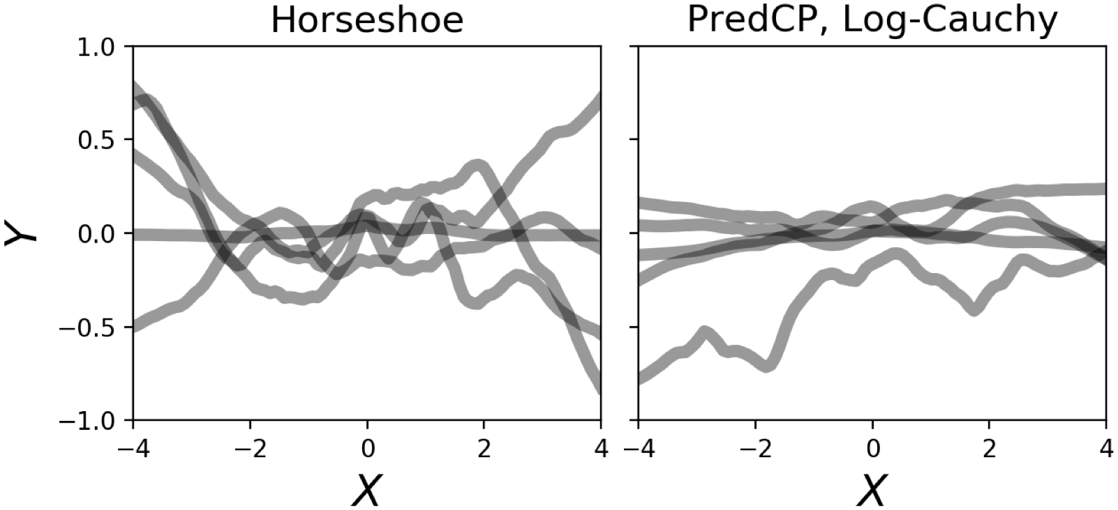
where denotes the response noise and is any positively homogeneous activation function (such as the ReLU). The crucial term represents the variance that the th layer’s transformation term contributes to the resnet’s prediction for . The expression makes clear that the PredCP is performing functional regularization: a zero-favoring will encourage this variance to be small. Dropout has been shown to curb the variance of hidden units in a similar way (Baldi and Sadowski 2013). Figure 3(b) shows functions sampled from a resnet with a horseshoe prior (left) and a depth-wise log-Cauchy PredCP (right). The PredCP’s samples are closer to linear due to the regularization of the predictive variance. Yet, recall that the log-Cauchy is heavy-tailed and therefore allows some functions to stray from the origin, as we see one sample has done.
5.2 Hierarchical Modeling for Meta-Learning
Meta-learning is another natural application for the PredCP as it can control the degree to which information is pooled across tasks. Following the approach of Chen et al. 2019, we use the generative model: where indexes the task, is data for the th task, are local parameters specific to the th task, and are global meta-parameters. The scale controls local adaptation, and as , the task structure becomes irrelevant. This hierarchical meta-learning model is perfectly suited for a PredPC as the global parameters define a natural reference model:
Computing the KLD between the original and reference models then quantifies the information lost when ignoring the task structure. The prior is written as:
| (12) |
where is shorthand for the expected KLD on the th task. In the experiments, we follow Chen et al. 2019’s modular specification by applying the PredCP layer-wise. Doing so allows the feature-extracting shallow layers to adapt to a different degree than the classification-based final layer.
| Variational Inference | Markov Chain Monte Carlo | |||||||
|---|---|---|---|---|---|---|---|---|
| Data Set | N | D | Half-Cauchy | ECP | PredCP | Half-Cauchy | ECP | PredCP |
| allaml | 51 | 7129 | ||||||
| colon | 44 | 2000 | ||||||
| breast | 82 | 9 | ||||||
6 RELATED WORK
Penalized Complexity Prior
Our work is directly inspired by and extends Simpson et al. 2017’s penalized complexity prior (PCP). Let denote a ‘base’ prior and an ‘extended’ prior, with controlling ’s expressivity. Simpson et al. 2017 define a prior for by placing a prior on the root-KLD and changing variables:
The major difference between the PCP and our PredCP is in how the KLD is formulated. Simpson et al. 2017 compute the divergence between priors whereas we use the divergence between data models . This crucial change is necessary since the PCP is hard to define for NNs and similarly complicated models. As the priors and the divergence are defined in -space, specifying the PCP still requires intimate knowledge of the parameters, running into the same challenges of high-dimensionality and unidentifiability. Because of our modification to -space, this makes the computation harder since we need to marginalize to work with . This difficulty necessitated the KLD upper bound in Equation 8. Another benefit of comparing the models in -space is that we can easily use point-mass priors for . Simpson et al. 2017 also do this, but because their KLD is defined on , they need to take limits. PCPs have been used as priors for P-splines (Ventrucci and Rue 2016), distributional regression (Klein and Kneib 2016), autoregressive processes (Sørbye and Rue 2017), mixed effects models (Ventrucci et al. 2019), and Gaussian random fields (Fuglstad et al. 2019).
Functional Priors for Bayesian NNs
Our work is also motivated by recent efforts to rethink prior specification for Bayesian NNs. As we truly care about the distribution over predictive functions, specifying functional priors has received much attention of late (Ma et al. 2019; Hafner et al. 2019; Flam-Shepherd et al. 2018; Louizos et al. 2019). The hope is that it is easier to reason about our preferences for functions than for parameters. However, existing functional priors introduce cumbersome byproducts into the Bayesian workflow. Placing a functional prior on a NN requires either taking infinite width limits (Pearce et al. 2019), optimizing divergences involving stochastic processes (Flam-Shepherd et al. 2017; Sun et al. 2019), or pre-training (Flam-Shepherd et al. 2017; Nalisnick and Smyth 2018; Atanov et al. 2019). Our framework, on the other hand, uses reparameterization to obtain a proper prior on the parameters, creating no complications for traditional Bayesian inference.
| Prior Type | boston | concrete | energy | kin8nm | power | wine | yacht |
|---|---|---|---|---|---|---|---|
| Fixed | |||||||
| Shrinkage | |||||||
| PredCP |
| Fewshot-CIFAR100 | Mini-ImageNet | |||
|---|---|---|---|---|
| 1-Shot | 5-Shot | 1-Shot | 5-Shot | |
| MAML | ||||
| -MAML + uniform prior | ||||
| -MAML + shrinkage prior | ||||
| -MAML + PredCP | ||||
7 EXPERIMENTS
We evaluate the PredCP on regression, classification, and few-shot learning tasks under a variety of algorithms for posterior inference. The experimental details are provided in the appendix. In all cases, we use relatively small data sets so that the prior’s influence is not overwhelmed by the likelihood.
Logistic Regression
We first report an experiment in which the ECP can be computed and posteriors obtained with high-fidelity. We use the logistic regression model: , , where denotes the logistic function and a half-Cauchy prior. We compare three priors for : , which is the default prior recommended by Gelman 2006 and Carvalho et al. 2009, the ECP (via probit approximation (Bishop 2006)), and the PredCP. The log-Cauchy is the KLD prior. We use Stan (Carpenter et al. 2017) to obtain the full posterior , performing both variational inference (Normal mean-field approximation) (Kucukelbir et al. 2017) and Hamiltonian MC. We test the priors on three small medical data sets (Golub et al. 1999; Alon et al. 1999; Patrício et al. 2018) so that the prior strongly influences the posterior. Furthermore, two of the data sets are high-dimensional () in order to test if the PredCP can prevent overfitting. Table 1 reports the predictive log-likelihood on the test set averaged over splits. The ECP and PredCP have comparable performance and outperform the half-Cauchy in four of six cases and with one tie.
Neural Networks
We next report results using resnets for regression: , , where indexes layers, rows of the weight matrix, and columns. This prior has two forms of Bayesian regularization. The row-wise scale implements automatic relevance determination (ARD) (MacKay 1994; Neal 1994), which controls the effective width. The layer-wise scale performs automatic depth determination (ADD) (Nalisnick et al. 2019), as it controls the effective depth. We again compare three strategies for setting . The first is to use a fixed scale (), thereby removing ADD and serving as a weak baseline. The second is to use a shrinkage prior. Nalisnick et al. 2019 use an inverse gamma prior, and we report their results as the strong baseline. For our method we use the PredCP with a log-Cauchy KLD prior. For posterior inference, we use Bayes-by-backprop (Blundell et al. 2015) for the weights and variational EM (Wu et al. 2019; Nalisnick et al. 2019) for the scales and . The maximization step cannot be performed analytically for the PredCP, as it can for the inverse gamma, and so we perform iterative gradient-based optimization. Again, we use relatively small data sets to ensure the prior remains influential: results on UCI benchmarks (Dua and Graff 2019; Hernández-Lobato and Adams 2015) are reported in Table 2. Using the PredCP results in the best test set root-mean-square error (RMSE) for three of the seven benchmarks (boston, energy, yacht) and in one tie (kin8nm).
Few-Shot Learning
Our final experiment evaluates the PredCP for few-shot learning. We follow Chen et al. 2019’s experimental framework, using the hierarchical model (described in Section 5) and their -MAML algorithm for optimization. In essence, -MAML performs MAP estimation for , , and . The classifier is the standard four-layer convolutional NN (Finn et al. 2017). We experimentally compare four different priors, each applied layer-wise (again following Chen et al. 2019). The first baseline is (improper uniform), which corresponds to standard MAML (Finn et al. 2017). The second baseline is Chen et al. 2019’s model, which uses the improper uniform prior for the meta-parameters: . For a third baseline, we extend Chen et al. 2019’s model by placing a shrinkage prior on , considering half-Cauchy, log-Cauchy, exponential, and gamma-exponential mixture distributions. Finally, our proposal is to place a PredCP on . We use the same four shrinkage priors for . We evaluate all priors on the few-shot CIFAR100 (Oreshkin et al. 2018) and mini-ImageNet (Vinyals et al. 2016) classification benchmarks, using the standard -way -shot and -shot protocols. Table 3 reports the results. The PredCP consistently improves accuracy across all experiments.
8 Conclusions
We proposed a novel prior termed the predictive complexity prior (PredCP). This prior is constructed procedurally and provides functional regularization. We found the PredCP to improve generalization across a range of small-data tasks that require careful regularization. The log-Cauchy served as a good default KLD prior. One potential avenue for future work is to re-introduce predictive correlations into the divergence function, as these were lost when switching to the upper bound (Equation 8). The resulting resnet-PredCP could then account for more interesting local structure in the predictive function, not just its point-wise variance. Another direction is to explore other divergences, including symmetric ones such as the Hellinger distance. Lastly, it would be interesting to investigate if the PredCP mitigates the misspecification issues described by Wenzel et al. 2020 or improves uncertainty estimation on out-of-distribution data.
References
- Alon et al. (1999) Uri Alon, Naama Barkai, Daniel A. Notterman, Kurt Gish, Suzanne Ybarra, Daniel Mack, and Arnold J. Levine. Broad Patterns of Gene Expression Revealed by Clustering Analysis of Tumor and Normal Colon Tissues Probed by Oligonucleotide Arrays. In Proceedings of the National Academy of Sciences, 1999.
- Antorán et al. (2020) Javier Antorán, James Urquhart Allingham, and José Miguel Hernández-Lobato. Variational Depth Search in ResNets. ICLR Workshop on Neural Architecture Search, 2020.
- Atanov et al. (2019) Andrei Atanov, Arsenii Ashukha, Kirill Struminsky, Dmitriy Vetrov, and Max Welling. The Deep Weight Prior. In Proceedings of the International Conference on Learning Representations, 2019.
- Baldi and Sadowski (2013) Pierre Baldi and Peter J. Sadowski. Understanding Dropout. In Advances in Neural Information Processing Systems, 2013.
- Bernardo (1979) Jose M Bernardo. Reference Posterior Distributions for Bayesian Inference. Journal of the Royal Statistical Society. Series B (Methodological), 1979.
- Bishop (2006) Christopher M. Bishop. Pattern Recognition and Machine Learning. Springer, 2006.
- Blundell et al. (2015) Charles Blundell, Julien Cornebise, Koray Kavukcuoglu, and Daan Wierstra. Weight Uncertainty in Neural Networks. In Proceedings of the 32nd International Conference on Machine Learning, 2015.
- Box (1980) George E. P. Box. Sampling and Bayes’ Inference in Scientific Modelling and Robustness. Journal of the Royal Statistical Society: Series A, 1980.
- Carpenter et al. (2017) Bob Carpenter, Andrew Gelman, Matthew D. Hoffman, Daniel Lee, Ben Goodrich, Michael Betancourt, Marcus Brubaker, Jiqiang Guo, Peter Li, and Allen Riddell. Stan: A Probabilistic Programming Language. Journal of Statistical Software, 2017.
- Carvalho et al. (2009) Carlos M. Carvalho, Nicholas G. Polson, and James G. Scott. Handling Sparsity via the Horseshoe. In Proceedings of the 12th International Conference on Artificial Intelligence and Statistics, 2009.
- Casella (1985) George Casella. An Introduction to Empirical Bayes Data Analysis. The American Statistician, 1985.
- Chen et al. (2019) Yutian Chen, Abram L. Friesen, Feryal Behbahani, David Budden, Matthew W. Hoffman, Arnaud Doucet, and Nando de Freitas. Modular Meta-Learning with Shrinkage. NeurIPS Workshop on Meta-Learning, 2019.
- Dikov and Bayer (2019) Georgi Dikov and Justin Bayer. Bayesian Learning of Neural Network Architectures. In Proceedings of the 22nd International Conference on Artificial Intelligence and Statistics, 2019.
- Dua and Graff (2019) Dheeru Dua and Casey Graff. UCI Machine Learning Repository, 2019.
- Finn et al. (2017) Chelsea Finn, Pieter Abbeel, and Sergey Levine. Model-Agnostic Meta-Learning for Fast Adaptation of Deep Networks. In Proceedings of the 34th International Conference on Machine Learning, 2017.
- Flam-Shepherd et al. (2017) Daniel Flam-Shepherd, James Requeima, and David Duvenaud. Mapping Gaussian Process Priors to Bayesian Neural Networks. NeurIPS Workshop on Bayesian Deep Learning, 2017.
- Flam-Shepherd et al. (2018) Daniel Flam-Shepherd, James Requeima, and David Duvenaud. Characterizing and Warping the Function Space of Bayesian Neural Networks. NeurIPS Workshop on Bayesian Deep Learning, 2018.
- Fuglstad et al. (2019) Geir-Arne Fuglstad, Daniel Simpson, Finn Lindgren, and Håvard Rue. Constructing Priors that Penalize the Complexity of Gaussian Random Fields. Journal of the American Statistical Association, 2019.
- Gal and Ghahramani (2016) Yarin Gal and Zoubin Ghahramani. Dropout as a Bayesian Approximation: Representing Model Uncertainty in Deep Learning. In Proceedings of the 33rd International Conference on Machine Learning, 2016.
- Gelman (2006) Andrew Gelman. Prior Distributions for Variance Parameters in Hierarchical Models. Bayesian Analysis, 2006.
- Gelman et al. (2017) Andrew Gelman, Daniel Simpson, and Michael Betancourt. The Prior Can Often Only Be Understood in the Context of the Likelihood. Entropy, 2017.
- Golub et al. (1999) Todd R. Golub, Donna K. Slonim, Pablo Tamayo, Christine Huard, Michelle Gaasenbeek, Jill P. Mesirov, Hilary Coller, Mignon L. Loh, James R. Downing, and Mark A. Caligiuri. Molecular Classification of Cancer: Class Discovery and Class Prediction by Gene Expression Monitoring. Science, 1999.
- Hafner et al. (2019) Danijar Hafner, Dustin Tran, Timothy Lillicrap, Alex Irpan, and James Davidson. Noise Contrastive Priors for Functional Uncertainty. In Proceedings of the 35th Conference on Uncertainty in Artificial Intelligence, 2019.
- He et al. (2016) Kaiming He, Xiangyu Zhang, Shaoqing Ren, and Jian Sun. Deep Residual Learning for Image Recognition. In Proceedings of the IEEE Conference on Computer Vision and Pattern Recognition, 2016.
- Heek and Kalchbrenner (2019) Jonathan Heek and Nal Kalchbrenner. Bayesian Inference for Large Scale Image Classification. ArXiv e-Prints, 2019.
- Hernández-Lobato and Adams (2015) José Miguel Hernández-Lobato and Ryan Adams. Probabilistic Backpropagation for Scalable Learning of Bayesian Neural Networks. In Proceedings of the 32nd International Conference on Machine Learning, 2015.
- Jeffreys (1946) Harold Jeffreys. An Invariant Form for the Prior Probability in Estimation Problems. In Proceedings of the Royal Society of London A: Mathematical, Physical and Engineering Sciences, 1946.
- Johnson and Rossell (2010) Valen E. Johnson and David Rossell. On the Use of Non-Local Prior Densities in Bayesian Hypothesis Tests. Journal of the Royal Statistical Society: Series B, 2010.
- Kingma and Ba (2014) Diederik Kingma and Jimmy Ba. Adam: A Method for Stochastic Optimization. In Proceedings of the International Conference on Learning Representations, 2014.
- Kingma and Welling (2014) Diederik Kingma and Max Welling. Efficient Gradient-Based Inference Through Transformations Between Bayes Nets and Neural Nets. In Proceedings of the 31st International Conference on Machine Learning, 2014.
- Klein and Kneib (2016) Nadja Klein and Thomas Kneib. Scale-Dependent Priors for Variance Parameters in Structured Additive Distributional Regression. Bayesian Analysis, 2016.
- Kucukelbir et al. (2017) Alp Kucukelbir, Dustin Tran, Rajesh Ranganath, Andrew Gelman, and David Blei. Automatic Differentiation Variational Inference. The Journal of Machine Learning Research, 2017.
- Louizos et al. (2019) Christos Louizos, Xiahan Shi, Klamer Schutte, and Max Welling. The Functional Neural Process. In Advances in Neural Information Processing Systems, 2019.
- Ma et al. (2019) Chao Ma, Yingzhen Li, and José Miguel Hernández-Lobato. Variational Implicit Processes. In Proceedings of the 36th International Conference on Machine Learning, 2019.
- Ma et al. (2018) Fangchang Ma, Ulas Ayaz, and Sertac Karaman. Invertibility of Convolutional Generative Networks from Partial Measurements. In Advances in Neural Information Processing Systems, 2018.
- MacKay (1994) David MacKay. Bayesian Non-Linear Modeling for the Prediction Competition. Maximum Entropy and Bayesian Methods, 1994.
- Nalisnick and Smyth (2018) Eric Nalisnick and Padhraic Smyth. Learning Priors for Invariance. In Proceedings of the 21st International Conference on Artificial Intelligence and Statistics, 2018.
- Nalisnick et al. (2019) Eric Nalisnick, José Miguel Hernández-Lobato, and Padhraic Smyth. Dropout as a Structured Shrinkage Prior. In Proceedings of the 36th International Conference on Machine Learning, 2019.
- Neal (1994) Radford M. Neal. Bayesian Learning for Neural Networks. PhD thesis, University of Toronto, 1994.
- Oreshkin et al. (2018) Boris Oreshkin, Pau Rodríguez López, and Alexandre Lacoste. TADAM: Task Dependent Adaptive Metric for Improved Few-Shot Learning. In Advances in Neural Information Processing Systems, 2018.
- Papamakarios et al. (2019) George Papamakarios, Eric Nalisnick, Danilo Jimenez Rezende, Shakir Mohamed, and Balaji Lakshminarayanan. Normalizing Flows for Probabilistic Modeling and Inference. ArXiv e-Prints, 2019.
- Patrício et al. (2018) Miguel Patrício, José Pereira, Joana Crisóstomo, Paulo Matafome, Manuel Gomes, Raquel Seiça, and Francisco Caramelo. Using Resistin, Glucose, Age and BMI to Predict the Presence of Breast Cancer. BMC Cancer, 2018.
- Pearce et al. (2019) Tim Pearce, Russell Tsuchida, Mohamed Zaki, Alexandra Brintrup, and Andy Neely. Expressive Priors in Bayesian Neural Networks: Kernel Combinations and Periodic Functions. In Proceedings of the 35th Conference on Uncertainty in Artificial Intelligence, 2019.
- Phuong and Lampert (2020) Mary Phuong and Christoph H. Lampert. Functional vs. Parametric Equivalence of ReLU Networks. In Proceedings of the International Conference on Learning Representations, 2020.
- Piironen and Vehtari (2017a) Juho Piironen and Aki Vehtari. On the Hyperprior Choice for the Global Shrinkage Parameter in the Horseshoe Prior. In Proceedings of the 20th International Conference on Artificial Intelligence and Statistics, 2017a.
- Piironen and Vehtari (2017b) Juho Piironen and Aki Vehtari. Sparsity Information and Regularization in the Horseshoe and Other Shrinkage Priors. Electronic Journal of Statistics, 2017b.
- Robert (2001) Christian Robert. The Bayesian Choice. Springer, 2001.
- Shin et al. (2018) Minsuk Shin, Anirban Bhattacharya, and Valen E. Johnson. Scalable Bayesian Variable Selection Using Nonlocal Prior Densities in Ultrahigh-Dimensional Settings. Statistica Sinica, 2018.
- Simpson et al. (2017) Daniel Simpson, Håvard Rue, Andrea Riebler, Thiago G. Martins, and Sigrunn H. Sørbye. Penalising Model Component Complexity: A Principled, Practical Approach to Constructing Priors. Statistical Science, 2017.
- Song et al. (2019) Yang Song, Chenlin Meng, and Stefano Ermon. MintNet: Building Invertible Neural Networks with Masked Convolutions. In Advances in Neural Information Processing Systems, 2019.
- Sørbye and Rue (2017) Sigrunn Holbek Sørbye and Håvard Rue. Penalised Complexity Priors for Stationary Autoregressive Processes. Journal of Time Series Analysis, 2017.
- Sun et al. (2019) Shengyang Sun, Guodong Zhang, Jiaxin Shi, and Roger Grosse. Functional Variational Bayesian Neural Networks. In Proceedings of the International Conference on Learning Representations, 2019.
- Ventrucci and Rue (2016) Massimo Ventrucci and Håvard Rue. Penalized Complexity Priors for Degrees of Freedom in Bayesian P-Splines. Statistical Modelling, 2016.
- Ventrucci et al. (2019) Massimo Ventrucci, Daniela Cocchi, Gemma Burgazzi, and Alex Laini. PC Priors for Residual Correlation Parameters in One-Factor Mixed Models. Statistical Methods & Applications, 2019.
- Vinyals et al. (2016) Oriol Vinyals, Charles Blundell, Tim Lillicrap, and Daan Wierstra. Matching Networks for One Shot Learning. In Advances in Neural Information Processing Systems, 2016.
- Wen et al. (2018) Yeming Wen, Paul Vicol, Jimmy Ba, Dustin Tran, and Roger Grosse. Flipout: Efficient Pseudo-Independent Weight Perturbations on Mini-Batches. In Proceedings of the International Conference on Learning Representations, 2018.
- Wenzel et al. (2020) Florian Wenzel, Kevin Roth, Bastiaan S. Veeling, Jakub Świątkowski, Linh Tran, Stephan Mandt, Jasper Snoek, Tim Salimans, Rodolphe Jenatton, and Sebastian Nowozin. How Good is the Bayes Posterior in Deep Neural Networks Really? In Proceedings of the 37th International Conference on Machine Learning, 2020.
- Wu et al. (2019) Anqi Wu, Sebastian Nowozin, Edward Meeds, Richard E. Turner, José Miguel Hernández-Lobato, and Alexander L. Gaunt. Deterministic Variational Inference for Robust Bayesian Neural Networks. In Proceedings of the International Conference on Learning Representations, 2019.
- Zellner (1986) A. Zellner. On Assessing Prior Distributions and Bayesian Regression Analysis with g-Prior Distributions. Bayesian Inference and Decision Techniques, 1986.
- Zhang et al. (2020) Ruqi Zhang, Chunyuan Li, Jianyi Zhang, Changyou Chen, and Andrew Gordon Wilson. Cyclical Stochastic Gradient MCMC for Bayesian Deep Learning. In Proceedings of the International Conference on Learning Representations, 2020.
Appendix A ECP FOR LINEAR REGRESSION, CONTINUED
A.1 Varying Prior Parameters
We consider the following priors on the KLD, denoted in the main text:
- •
- •
- •
Since the gamma prior favors and the exponential , we also consider a mixture of the two:
This mixture should achieve the same interpolation behavior as the log-Cauchy, balancing preferences for and . See Figure 4(a) for a visualization of the ECP for the gamma-exponential mixture as the mixing coefficient is varied. Figure 4(b) shows the log-Cauchy ECP as its scale is varied.
A.2 Dynamic Shrinkage Profile
One method for illuminating and comparing the effects of shrinkage priors is through their corresponding shrinkage profile (Carvalho et al. 2009). Consider the model: , , . Given one observation , the Bayes estimator for is: , . Making the change of variables , we can examine the induced prior . If places high density near , then the prior provides strong regularization since the Bayes estimator would be near zero. Conversely, a strong mode at means the resulting estimator would be near , implying a tendency to follow the data. Figure 4(c) shows the shrinkage profile for the log-Cauchy ECP for , comparing the profiles of the horseshoe’s. The horseshoe is an effective prior for robust regression since it is designed to equally favor and ( Beta). The shrinkage profile for the log-Cauchy also can place density at both extremes. However, unlike the horseshoe, the ECP enables dynamic shrinkage, being able to adjust the profile as a function of . We see that for , the log-Cauchy ECP actually favors the unshrunk solution whereas for strong shrinkage is preferred. The mixture ECP’s shrinkage profile is shown in Figure 4(d). Due to the exponential not having a heavy tail, the mixture ECP’s profile cannot place any significant density at , meaning that the model can never completely ‘forget’ the shrinkage regularization.


A.3 Example: Multivariate Regression
We now examine the case of multivariate regression: , where is an -dimensional vector of responses, the design matrix, and a vector of parameters. Using the multivariate analogs of the priors from above—, —we can derive the following ECP:
| (13) |
where denotes the trace operation and the determinant. The KLD is computed between and . We omit the details of the volume term due to space constraints.
Here the KLD is a multidimensional integral that takes into account correlations in the model’s predictions. Hence, we can explore how characteristics of the design matrix influence the prior. We consider the tail probability since, as probability mass moves away from the origin, the ECP increasingly prefers the extended model. Below we describe simulations using the mixture ECP due to its mixing weight being interpretable. First consider the case in which has a rank of one and all row vectors have a length of one. This means that the data is essentially redundant, generating the same predictions. As the rank of increases, the predictions start to become varied and the model output becomes responsive to each . Thus, we should expect to favor larger values as the rank of increases. Indeed, this is exactly the behavior we observe in Figure 4(e), plotting the tail probability as we vary the rank from to . Another attribute of we can vary is its scale: . Subfigure 4(f) shows the tail probability as the scale increases (for full-rank ). We find that scale changes result in more pronounced tail effects than changes in rank.
A.4 Example: ECP for the Linear Regression Coefficient
In the main text, we consider applying the ECP to the scale of the prior on , the regression coefficients. Yet, we can also define the ECP on directly. Consider the linear model , . We wish a define the ECP on to control deviation from the base model :
| (14) |
where is the response noise. Figure 5(a) shows three choices for —exponential (green), gamma (purple), and log-Cauchy (red)—and Figure 5(b) shows the prior each induces on . We see that choice of is significant. If places too little density at zero, the volume term in the ECP dominates, driving to zero at . In turn, this drives from reflecting the behavior of and suppresses any regularization. We see this behavior from the exponential (green) as its ECP has no density at zero. At the other end of the spectrum is the gamma (purple). It places too much density at zero, forcing to preference the base model . Lastly, the log-Cauchy (red) has the most interesting behavior: it has strong shrinkage at the origin to reflect but also significant density away from zero to represent . Hence the log-Cauchy is able to balance preferences for both and , interpolating between the exponential and gamma’s single-mindedness. Lastly, Figure 5(c) shows how changes as is varied—the data adaptive nature mentioned above. The ECP’s shrinkage is adjusted to the scale of the features, applying stronger regularization when is large and relaxing as decreases. This is sensible since the models predictions cannot change as drastically for small s as they can for large s.
Connection to Non-Local Priors
Perhaps the (log-Cauchy and mixture) ECP’s most interesting feature is in how it balances between and through multi-modality. In addition to the strong mode at zero, there are modes separated from and symmetric about the origin; see Figure 5(d). This is the defining feature of so-called non-local priors (Johnson and Rossell 2010). This class of priors is designed to achieve good convergence rates in Bayesian hypothesis testing by carefully allocating density exactly at the null and distinctly away from the null to represent the alternative. Shin et al. 2018 apply this non-local principle to Bayesian variable selection in high-dimensional regression via the following prior:
| (15) |
where is the linear model’s coefficient and is known as a product (2nd) moment prior (Johnson and Rossell 2010). See Figure 5(f) for a visualization. While the ECP and non-local prior have clear similarities, the connection can be made explicit my considering the Bayes factor , which is what we would use to test vs . The ECP’s KLD term contains this exact expression: which can be interpreted as the (log) Bayes factor expected if the data is truly generated by the extended model.


Appendix B BIJECTIVITY CONDITIONS FOR NEURAL NETWORKS
Below we show that is bijective w.r.t. for Gaussian and categorical observation models, ReLU activations, and Gaussian weight priors . We assume the base model has weights , where is the prior mean of the expanded model. In turn, the change of variables is well-defined and the PredCP is proper (i.e. integrates to ) when used in the applications given in Section 5. Before diving into the technical details, we point out that invertibility should not be hard to guarantee since is a scalar. If the reader is familiar with the literature on normalizing flows (Papamakarios et al. 2019) and invertible architectures (Song et al. 2019), one may have the impression that invertibility is hard to guarantee for neural networks, often requiring constraints on the weights. This is only the case because an invertible architecture must preserve bijectivity w.r.t. the entire input vector. We, to the contrary, just have to preserve scalar information. Moreover, we know this scalar is strictly positive, which eliminates any symmetry about the origin. Thus, intuitively, the information about should be preserved at every hidden layer as long as at least one ReLU unit is active. This brings up the only assumption that we require: non-degeneracy. That is, for every hidden layer, there must be at least one active ReLU unit (i.e. a unit evaluated to a positive value). This is an extremely weak assumption, especially for all but the smallest neural networks, and ReLU networks commonly satisfy much stronger non-degeneracy assumptions (Phuong and Lampert 2020). If dead layers would arise for some reason, initializing the biases to be positive should prevent the pathology. Before moving on to the main results, we first introduce two conventions.
Non-Centered Parameterization:
We assume all weights are represented in the observation model using the following non-centered form: , . This parameterization is useful for ‘exposing’ so that we can write the KLD as an explicit function of .
Linear Representation of ReLU Activations
Recall that feedforward networks with ReLU activations are piecewise-linear functions. Thus, it is equivalent to express a dense ReLU layer in terms of a diagonal ‘gating’ matrix (Ma et al. 2018):
| (16) |
otherwise . Using this convention, we can then represent the network’s linear output as:
where is a matrix containing the network’s linear output (i.e. before a softmax is applied, in the classification setting) for all training features .
B.1 Gaussian Observation Model
Let’s now consider checking for bijectivity w.r.t. when the observation model is Gaussian, i.e. . The expected KLD is then:
| (17) |
where indexes the training features and the output dimensions. Since does not involve , we can treat is as a constant. The sum over and forms a conic combination. Therefore if all terms have the same monotonicity and are bijective, then the sum will be bijective as well.
We first turn toward the expectation in the middle term and expand it using the non-centered parameterization. We drop the indexes to help with notational clutter:
| (18) |
Pushing through the expectation, we have:
Considering the first term, we have that if . For the second, . Thus, reduces to the first term, and since this term depends only on the prior means, it is equivalent to the output of the base model:
| (19) |
Now turning to the other expectation term in Equation 17 and using the expansion from Equation 18, we have:
The middle term drops out after taking the expectation. We are left with the two remaining terms:
We use the variables and to denote these two terms from here forward. They have the following three properties that will come in handy below. Firstly, their values are strictly positive due to the square and non-degeneracy assumption ( ). We emphasize this by giving them the superscript . Secondly, we know their derivative w.r.t. is zero. This is true for because it depends on only through and therefore only through the sign function. For , it does not depend on ; we have factored it out already. Thirdly, and are bounded w.r.t. . We know this in the former case because, again, controls only the ‘gates’ in and is bounded. The latter case is trivial due to not being a function of . Now substituting back into Equation 17, we have
| (20) |
All that is left to do is to check for injectivity and surjectivity. For the former, we need to verify the derivative has a constant sign, and we find that:
Clearly, the derivative is always positive, meaning the function is strictly increasing. Lastly, for surjectivity, it is sufficient to check that
As , we have that , therefore causing the first and last terms to cancel. The remaining term is then forced to zero simply by going to zero. As , the second term is sufficient for the full quantity to go to infinity since all other terms are bounded as a function of .
B.2 Categorical Observation Model
In the previous subsection, we showed that bijectivity is preserved at least up through the neural network’s linear output . We now consider the case of a categorical observation model. This case is harder to show explicitly because the expectation cannot be pushed through to individual terms as we did above. Rather, we base the argument on the fact that compositions of bijections form a bijection. In particular, given that is bijective, we need the three following operations to preserve that bijectivity: .
First considering the softmax, the softmax function is defined as:
where , , , and . We want to prove that the softmax is invertible w.r.t. the scale for fixed . Since is a scalar, it suffices that only one need be invertible. Below we show bijectity by showing injectivity and then surjectivity. We can show injectivity by examining the softmax’s derivative w.r.t. and showing it has a constant sign:
where the first term is positive and the second could be positive or negative, depending on the values. Denoting the maximum element of as , the derivative in this dimension is:
and now we know the second term is strictly positive since is a convex combination of . That is, assuming that there’s at least one , then . Conversely, for , we have:
![[Uncaptioned image]](2006.10801v3/softmax_wrt_tau.png)
since . Thus, we have that at least two dimensions—those corresponding to and —of the softmax are injective w.r.t. . For surjectivity, it is sufficient to check the limits. For , (), and for , we have and . Thus, is strictly decreasing on and that is strictly increasing on . In turn, Softmax: is a bijection. The figure to the right shows the softmax outputs for one particular setting of ; each line represents an output . We see that the blue ( and red () lines, the max and min dimensions respectively, are strictly monotonic. On the other hand, the orange line () is clearly not bijective since it doesn’t pass the horizontal line test.
On to the KLD, is strictly convex w.r.t. for fixed . This is indeed our setting since only is a function of . This strict convexity implies that has a unique, global minimum at and is strictly increasing as —and hence, is bijective. Lastly, the expectation does not have an analytical solution, and thus here (as well as in practice), we consider the Monte Carlo approximation:
where the approximation becomes exact as . The Monte Carlo approximation is a weighted sum of bijective, strictly increasing functions and therefore is also strictly increasing and bijective.
B.3 Residual Networks
The preceding two sections hold as well for residual networks. In fact, residual networks allow us to relax the non-degeneracy assumption. That is, for invertibility w.r.t. , we can have for just so long as there is a path of skip (identity) connections from layer to layer . This identity path preserves the information about that would be lost due to .
Appendix C DRAWING SAMPLES FROM THE PREDCP
The user may want to draw samples from the PredCP—for instance, to perform a prior predictive check (Box 1980). In general, sampling from a reparameterized model can be done via: , where is the base distribution and is the transformation (Papamakarios et al. 2019). Applying this formula to the PredCP, in theory, we could draw samples via:
| (21) |
where represents a sampled value of and represents an inversion of the expected-KLD, yielding as a function of . Unfortunately, the analytical inverse of is not available in general. Instead, we use the numerical inversion technique proposed by Song et al. 2019. See Algorithm 1 below.
We used Algorithm 1 to sample from the depth-wise PredCP and ancestral sampling to draw functions from the NN. We considered both residual and non-residual architectures, both having batch normalization applied at each hidden layer. The observation model is Gaussian with . We used a log-Cauchy KLD prior, , , and Monte Carlo samples for the expectation. In Figure 6, we show function samples for the standard Normal, horseshoe (), and PredCP for and hidden layers. The PredCP’s samples are notably simpler.

Appendix D MODULAR PRIOR SPECIFICATION FOR META-LEARNING
We provide details for specifying and evaluating modular priors for meta-learning. Following Chen et al. 2019, we split into distinct modules (e.g., layers), such that . Our goal is then to place a separate prior on each module, and allow the modules to adapt differently to new tasks. Denoting and as the global parameters and shrinkage parameter of module , respectively, we have that for the local parameters of task at module . By specifying , we can control how much each module is allowed to deviate from the global model. For example, Chen et al. 2019 place an improper flat prior on and perform MAP estimation. Importantly, to perform MAP estimation for , we need only evaluate the log density of the priors , and add these terms to the outer-loop optimization objective (Chen et al. 2019).
Defining a PredCP Prior for
In this setting, It is natural to consider the global parameters as defining the base model for the PredCP prior. We can achieve this by specifying the prior to be . Denoting , we then have
where we denote as the predictions made by the model using only global parameters. Next, for every module , we can define the extended model
where we use the notation to denote the model that uses for all but module , which uses . Using the notation from the main text, we further denote and . Recall that using the KLD upper bound, the PredCP prior for this setting can be expressed as
We can approximate the intractable term inside without bias via Monte-Carlo sampling:
where . Note that the KLD term itself is a sum over the KLD terms for each in the support set. In turn, each of these terms is a KLD between categorical likelihoods, which is easily computed. As detailed in the main text, we divide the sum by the number of points in the set to ease the reasoning about the parameters of . We can further achieve an unbiased estimator to the term inside using stochastic mini-batches of tasks, as is standard in the few-shot classification literature.
Finally, assuming a factorization of the ’s, we can simply evaluate the log-density for each prior, and compute their sum. In practice, we use single-sample estimators of the KL term, and compute the prior terms over batches of tasks to reduce the number of forward passes through the network required to compute the objective. The procedure for evaluating the PredCP prior for a batch of tasks is detailed in Algorithm 2. Here we use the notation to denote a forward pass through a convolutional neural network using a set of parameters, applied to an input. We treat the output of such a call as the logits of a categorical distribution.
Appendix E LOGISTIC REGRESSION EXPERIMENTAL DETAILS
For the logistic regression experiment in Section 6 (Table 1), we used the probabilistic programming language Stan (Carpenter et al. 2017) for the implementation of both Markov chain Monte Carlo (MCMC) and variational inference (VI) (Kucukelbir et al. 2017). In both cases, we performed inference for the full posterior . Following Piironen and Vehtari 2017a’s implementation, we used a non-centered parameterization: , . For MCMC, we left Stan at its default settings. We evaluated the predictive log-likelihood using posterior samples (the default output). For VI, Stan uses a mean-field Normal posterior, appropriately transforming all variables so that their support is . Again we left all hyper-parameters at their defaults. The predictive log-likelihood was evaluated with samples drawn from the approximate posterior. For the PredCP, we used samples to evaluate the Monte Carlo expectation over for colon and breast. For allaml, we used only one Monte Carlo sample due to the data set being larger and requiring more time to run the MCMC. The allaml and colon data sets were downloaded from http://featureselection.asu.edu/datasets.php. breast was downloaded from https://archive.ics.uci.edu/ml/datasets/Breast+Cancer+Coimbra. We standardized the features using the z-transform , which we found to improve the speed at which the MCMC converged. We made % - % train-test splits for all three data sets. We left out % of the training set for each as a validation set that we ultimately did not use.
Appendix F RESNET EXPERIMENTAL DETAILS
For the resnet regression experiment in Section 6 (Table 2), we followed the experimental framework of Nalisnick et al. 201955 5 https://github.com/enalisnick/dropout_icml2019 (which followed Gal and Ghahramani 2016 and Hernández-Lobato and Adams 2015). All networks had two hidden layers, ReLU activations, and no batch or layer normalization. The posterior was approximated as:
| (22) |
The weight approximation (Bayes-by-backprop (Blundell et al. 2015), fully factorized Gaussian) was optimized using Adam (Kingma and Ba 2014) with a learning rate of (other parameters left at Tensorflow defaults), using mini-batches of size , and run for epochs. The Monte Carlo expectations in the ELBO and PredCP both used samples and flipout (Wen et al. 2018) for decorrelation. The ARD scales could be updated in closed-form for all models. The PredCP does not allow for a closed-form update (for ADD) and so we used an iterative maximization step. We used only one step per update so that the PredCP’s training time was comparable to the other models’. The UCI data sets were standardized and divided into 20 % - % train-test splits, following Hernández-Lobato and Adams 2015. The test set RMSE was calculated using samples from the posterior. For the fixed scale model, we selected the better performing of . For the PredCP, we used the log-Cauchy KLD prior, finding it worked well in the logistic regression experiment and generated sensible sample functions. In Algorithm 3, we provide pseudo-code for evaluating the depth-wise (log) PredCP.
Appendix G FEW-SHOT CLASSIFICATION: EXPERIMENTAL DETAILS AND ADDITIONAL RESULTS
We provide experimental details and results for our few-shot classification experiments.
G.1 Data Details
We use two standard few-shot classification benchmarks for our experiments: mini-ImageNet (Vinyals et al. 2016) and few-shot CIFAR100 (FC; (Oreshkin et al. 2018)). For mini-ImageNet, images are first down-sampled to 84x84, and then normalized. For FC, the images are classified in their 32x32 format after normalization. We use the standard split as suggested by Vinyals et al. 2016 for mini-ImageNet, containing 64 training classes, 16 validation classes, and 20 test classes. For FC, we follow the protocol proposed by Oreshkin et al. 2018, using the CIFAR100 super-classes to split the data. See Oreshkin et al. 2018 supplementary for full details. An , task is randomly sampled according to the following procedure:
- •
Sample classes from the appropriate set uniformly at random.
- •
For each class, sample examples uniformly at random for the context / support set.
- •
For each class, sample examples uniformly at random for the target / query set.
Evaluation is conducted by randomly sampling 600 tasks from the test set. Average accuracy and standard errors are reported.
G.2 Network Architectures
For all tasks, we use the standard convolutional architecture proposed by Finn et al. 2017. Each network is comprised of four convolutional blocks, followed by a linear classier. For mini-ImageNet, we use a standard 3x3 convolution with 32 channels, followed by a max-pool (stride 2), a ReLU non-linearity, and a batch normalization layer. We flatten the output of the final layer, leading to an 800d representation, which is then passed through the linear classifier.
For FC, we employ the same architecture, but with 64 channels, and no max-pooling. A global-average pooling is applied to the output of the final convolutional layer, resulting in a 64d representation, which is then passed through the linear classifier.
We used the standard hyper-parameters proposed by Finn et al. 2017, without any tuning. In particular, we use 5 gradient steps for the inner loop during training, and 10 at test time. The inner learning rate is fixed to 0.01, and the meta-learning rate is 1e-3. We use a meta-batch size of 4, and train all models for 60,000 iterations.
G.3 Hyper-Priors and Additional Results
| Beta | Half-Cauchy | Log-Cauchy | Gem | Exponential | ||||
| 1-shot | 5-shot | 1-shot | 5-shot | 1-shot | 5-shot | 1-shot | 5-shot | |
| PredCP | ||||||||
| 1e-0 | 33.2 1.8 | 51.7 0.9 | 37.7 1.7 | 51.8 0.9 | 37.9 1.9 | 52.0 0.97 | 38.9 1.8 | 51.4 1.0 |
| 1e-1 | 39.6 1.6 | 51.4 0.9 | 37.9 1.9 | 50.6 0.7 | 40.9 1.8 | 51.7 0.9 | 39.5 1.9 | 51.1 0.8 |
| 1e-2 | 38.2 1.8 | 50.9 0.8 | 40.1 1.9 | 52.5 0.9 | 37.8 1.8 | 51.6 0.8 | 40.3 1.9 | 49.1 1.1 |
| 1e-3 | 39.7 1.9 | 52.9 0.9 | 40.2 1.8 | 50.6 1.0 | 38.8 1.8 | 51.3 0.9 | 38.5 1.8 | 50.8 0.9 |
| 1e-4 | 37.4 1.7 | 52.7 0.9 | 37.7 1.8 | 50.5 0.9 | 35.8 1.7 | 51.5 0.9 | 41.2 1.8 | 50.9 0.9 |
| Shrinkage Priors | ||||||||
| 1e-0 | 36.9 1.8 | 51.4 0.9 | 39.5 1.9 | 52.2 1.1 | 39.8 1.8 | 52.4 0.9 | 39.4 1.8 | 52.6 0.7 |
| 1e-1 | 39.8 1.9 | 52.7 0.8 | 40.9 1.9 | 52.7 0.9 | 36.6 1.8 | 52.5 0.8 | 38.7 1.9 | 51.6 1.1 |
| 1e-2 | 38.2 1.8 | 52.0 0.9 | 38.8 1.7 | 51.2 0.8 | 36.4 1.8 | 51.4 0.9 | 39.1 1.9 | 52.2 0.9 |
| 1e-3 | 39.3 1.7 | 51.3 0.7 | 35.9 1.8 | 50.8 0.9 | 40.8 1.9 | 51.9 1.0 | 37.5 1.9 | 52.2 0.8 |
| 1e-4 | 38.6 1.7 | 51.5 0.9 | 40.9 1.8 | 50.1 0.9 | 38.8 1.8 | 51.8 0.9 | 40.1 1.8 | 51.4 0.9 |
| MAML (flat prior) | 35.6 1.8 | 50.3 0.9 | ||||||
| MAML (flat prior) | 39.3 1.8 | 51.0 1.0 | ||||||
| Beta | Half-Cauchy | log-Cauchy | GEM | Exponential | ||||
|---|---|---|---|---|---|---|---|---|
| 1-shot | 5-shot | 1-shot | 5-shot | 1-shot | 5-shot | 1-shot | 5-shot | |
| PredCP | ||||||||
| 1e-0 | 33.4 1.7 | 60.7 0.8 | 28.6 1.6 | 59.8 0.8 | 28.7 1.6 | 59.1 0.8 | 30.2 1.7 | 59.1 0.8 |
| 1e-1 | 47.9 1.7 | 60.4 0.9 | 49.3 1.7 | 60.4 0.7 | 47.5 1.9 | 61.4 0.8 | 47.7 1.7 | 60.6 0.9 |
| 1e-2 | 47.0 1.8 | 60.3 0.7 | 45.9 1.6 | 60.7 0.8 | 46.7 1.8 | 61.7 0.7 | 47.2 1.9 | 61.9 0.9 |
| 1e-3 | 46.4 1.7 | 61.3 0.8 | 48.1 1.8 | 61.2 0.9 | 47.9 1.7 | 60.5 0.8 | 46.9 1.7 | 60.5 0.8 |
| 1e-4 | 47.7 1.8 | 60.4 0.9 | 47.7 1.8 | 60.3 0.9 | 48.1 1.9 | 60.1 0.9 | 48.3 1.8 | 60.4 0.9 |
| Shrinkage Priors | ||||||||
| 1e-0 | 42.9 1.8 | 57.3 0.9 | 48.5 1.7 | 60.9 0.9 | 24.7 1.5 | 29.0 0.7 | 44.5 1.8 | 57.8 0.9 |
| 1e-1 | 46.5 1.8 | 59.2 0.9 | 47.2 1.8 | 59.7 0.9 | 45.8 1.8 | 58.7 0.8 | 47.0 1.8 | 59.6 0.9 |
| 1e-2 | 46.8 1.7 | 59.3 0.8 | 46.3 1.9 | 59.3 0.8 | 46.7 1.7 | 60.1 0.7 | 46.8 1.8 | 59.1 0.9 |
| 1e-3 | 47.3 1.9 | 59.2 0.9 | 47.7 1.7 | 59.3 0.9 | 47.2 1.9 | 60.1 0.9 | 47.5 1.9 | 59.5 1.0 |
| 1e-4 | 46.7 1.8 | 59.2 0.9 | 47.4 1.7 | 60.2 0.7 | 48.0 1.5 | 59.5 0.9 | 47.8 1.7 | 58.6 0.9 |
| MAML (flat prior) | 45.6 1.8 | 58.4 0.9 | ||||||
| MAML (flat prior) | 47.4 1.8 | 60.1 0.9 | ||||||
For the modular shrinkage model, we experiment with four hyper-priors: Half-Cauchy, log-Cauchy, a mixture of Gamma and Exponential (GEM), and standard Exponential. Each of these is experimented with as a standard shrinkage prior, as well as the base prior for the PredCP. The parameters of the hyper-priors are fixed throughout experimentation, and are given as follows:
- •
Half-Cauchy:
- •
Log-Cauchy:
- •
GEM:
- •
Exponetial:
Additionally, we experimented with a vague (flat) prior, which recovers the model proposed by Chen et al. 2019. In addition, we also add a constant weight , which multiplies the prior on in the outer-loop objective for both the regular shrinkage and PredCP. For each prior, we experiment with .