Warping Wormholes with Dust:
a Metric Construction of the Python’s Lunch
Ning Bao,a,b Aidan Chatwin-Davies,c and Grant N. Remmenb
aComputational Science Initiative
Brookhaven National Laboratory, Upton, New York, 11973
bCenter for Theoretical Physics and Department of Physics
University of California, Berkeley, CA 94720 and
Lawrence Berkeley National Laboratory, Berkeley, CA 94720
cKU Leuven, Institute for Theoretical Physics
Celestijnenlaan 200D B-3001 Leuven, Belgium ††
e-mail: ningbao75@gmail.com, aidan.chatwindavies@kuleuven.be, grant.remmen@berkeley.edu
Abstract
We show how wormholes in three spacetime dimensions can be customizably warped using pressureless matter. In particular, we exhibit a large new class of solutions in -dimensional general relativity with energy-momentum tensor describing a negative cosmological constant and positive-energy dust. From this class of solutions, we construct wormhole geometries and study their geometric and holographic properties, including Ryu-Takayanagi surfaces, entanglement wedge cross sections, mutual information, and outer entropy. Finally, we construct a Python’s Lunch geometry: a wormhole in asymptotically anti-de Sitter space with a local maximum in size near its middle.
1 Introduction
Much progress has been made over the past fifteen years in the study of the intricate relationship between quantum information theory and quantum gravity, especially within the context of the Anti-de Sitter/Conformal Field Theory (AdS/CFT) correspondence [1, 2, 3]. Holographic dualities between information theoretic quantities and bulk geometric quantities form a central part of this program, the most prominent perhaps being the duality between extremal surface area and entanglement entropy [4, 5]. Proposals for the holographic duals of myriad other entropic quantities have since followed, as well as conjectures about the holographic dual of entanglement itself [6] and other information theoretic quantities, such as computational complexity [7, 8, 9].
Exact gravitational solutions provide rich bottom-up tests and insight into holographic proposals and conjectures away from the AdS vacuum. In this work, we present a new class of asymptotically AdS spacetimes in dimensions that contain pressureless dust, with a spatial distribution that is straightforwardly customizable; see Eqs. (3) and (4). Moreover, for suitable choices of the distribution, one can fold up slices of these spacetimes into two-sided wormholes that have irregular profiles in their throats. Among this new class of spacetimes, we will find that the dust distribution can be engineered so as to generate a concrete implementation of a “Python’s Lunch,” a special type of wormhole proposed in and sketched in Fig. 1, which will allow our classical construction to make contact with recent investigations into holographic complexity.
The question of quantum mechanical complexity associated with gravitational systems has been of interest for some time in the context of black holes and holography. In Ref. [11], Harlow and Hayden argued that certain tasks, in particular the distillation of a Bell pair’s worth of information from Hawking radiation, is exponentially hard in the evaporating black hole’s entropy. However, the subsequent “complexity equals action” conjecture of Refs. [7, 8, 9] generated tension with this argument. According to the conjecture, given a holographic CFT state that is dual to a two-sided black hole, such as the thermofield double, its computational complexity is dual to the length of the wormhole or to the value of the gravitational action within the Wheeler-DeWitt patch. However, the Harlow-Hayden proposal can be reformulated as the protocol necessary to prepare the thermofield double state by acting on the two CFTs in a separable manner, where one of the CFTs plays the role of the black hole and the other the emitted Hawking radiation. On these grounds, one therefore concludes that the complexity of the thermofield double state is very large, while the complexity equals action proposal yields a much smaller value given by the gravitational action.
The Python’s Lunch proposal of Ref. [10] suggested that the source of this discrepancy could be the restriction that the computation described by only makes use of computational gates that act on the two CFTs (or equivalently, the two sides of the wormhole) in a separable manner, i.e., not in a coupled fashion. In other words, the complexity that appears in the Harlow-Hayden protocol is a restricted complexity, which could clearly be much larger than an “unrestricted” complexity measured by gravitational action. The Python’s Lunch was then offered as an example to support this resolution with starker geometric intuition.
In essence, a Python’s Lunch geometry is an asymptotically AdS wormhole with a bulge in its throat. A spacelike slice of such a wormhole has a local maximum in its width near the middle of the throat, with local minima on either side, as illustrated in Fig. 1.11 1 A related concept is Wheeler’s “bag of gold” spacetime; see and refs. therein. While the bag of gold requires a high degree of symmetry to stitch the FRW cosmology onto a Schwarzshild black hole throat, the Python’s Lunch construction we will explore will not require this constraint. The region in between the local minima is difficult to access from one boundary alone, in the sense that once such a narrow waist exists that is homologous to an entire boundary, minimal boundary-anchored objects do not probe past the waist. Provided that small numbers of individual computational operations on a single boundary correspond to bulk operations with negligible backreaction in the region swept out by boundary-anchored probes, it would therefore take a large number of such operations to probe the inner region. In other words, the probes for which it is easy to access the inner region are those probes that are anchored to both boundaries.
This proposal is compelling, and so it is desirable to explicitly construct Python’s Lunch geometries that go beyond the special-case constructions and tensor network analogies discussed in . Moreover, because tensor networks have known limitations in their abilities to reproduce bulk geometry [13, 14], it is all the more worthwhile to find a more general and explicit construction of a class of spacetime metrics capable of describing a Python’s Lunch.
While we will arrive at postprandial pythons in the end, let us step back to the beginning and study the preprandial geometries that we initially advertised. In Sec. 2, we will motivate and derive the dust geometries we will consider in the remainder of the paper, in particular understanding its metric and geodesic behaviors for the case of a step-function dust distribution. In Sec. 3, we will construct a wormhole by cutting and pasting together portions of these dust geometries. In Sec. 4, for our step-function dust wormhole, we will investigate the entanglement wedge phases and calculate the well-studied entanglement wedge cross section and mutual information [17, 18, 19, 20], as well as the outer entropy [21, 22]. Finally, using the intuition gained from the step-function ansatz, in Sec. 5 we will explicitly engineer a Python’s Lunch geometry using a different dust distribution. In particular, we will numerically compute the wormhole diameter along its length and the entanglement wedge cross section. We discuss future directions and conclude in Sec. 6.
2 Geometries for AdS plus dust
We begin by deriving a new asymptotically AdS solution to the Einstein equation in 2+1 dimensions that contains pressureless dust. After writing down the metric in Sec. 2.1, we find the spacelike boundary-anchored geodesics for a simple dust distribution in Sec. 2.2.
2.1 Metric
Consider the Einstein equation for a three-dimensional spacetime with negative cosmological constant plus dust,22 2 Throughout, we work with mostly-plus metric signature, sign conventions and , and, unless otherwise specified, set .
| (1) |
where the only nonzero component of is and we have written the cosmological constant as . When , one has the solution, which we write in Poincaré patch coordinates as
| (2) |
where the boundary is located at .
When the dust density is not zero, but instead , we find that the class of metrics
| (3) |
is a solution to the Einstein equation (1). Here, the dust density satisfies the differential equation
| (4) |
where we use ′ to denote . We believe that this represents a new, large class of exact solutions to the Einstein equation; it does not appear explicitly in, e.g., Ref. [23] or among the metrics considered in and refs. therein.
The Cotton-York tensor has nonzero components and . Defining the unit timelike vector , the traceless Ricci tensor can be written as . Thus, in the notation of Refs. [23, 25], these spacetimes have a Cotton tensor that is a special case of Petrov type , with one eigenvalue vanishing, and have a traceless Ricci tensor of Petrov type .
We see that is -independent and, on slices of constant , this metric looks like a warped version of hyperbolic space, with warp factor . It might be desirable to set , so that on constant- slices the coordinate in Eq. (3) can be identified with the -coordinate in the hyperbolic plane in Eq. (2). For any desired density profile of , one then solves the differential equation for to obtain the metric at constant , then stitches together the solutions for arbitrary .
The metric (3) is time-reflection symmetric about , since is even. Thus, taking the slice, we can apply the Ryu-Takayanagi (RT) formula to compute entropies of boundary regions by finding minimal spacelike geodesics. The overall time-dependent factor in Eq. (3), which vanishes when , is reminiscent of FRW cosmologies written in conformal time, and indeed one could choose coordinates in which Eq. (3) represents a dust distribution that expands from a big bang, comes to rest at , and recollapses to a big crunch.
It will be well motivated to take , so that and coincide. Defining , for each value of we have the homogeneous, linear, second-order ordinary differential equation:
| (5) |
Defining , we can recast this as
| (6) |
Note that this is precisely the time-independent one-dimensional Schrödinger equation,
| (7) |
with the identifications
| (8) | ||||
This allows us to generate a large number of nontrivial dust solutions by directly translating solutions to the Schrödinger equation using the dictionary in Eq. (8). Interestingly, the energy condition corresponds with the requirement that , i.e., a “classical”-like, oscillatory solution, viewing Eq. (8) in a WKB context.
Let us solve Eq. (6) for the example density profile
| (9) |
i.e., empty AdS at small and constant dust density at . The comoving density of the dust is ; we require the dust to be of positive mass density, so . Similarly, the comoving density and pressure associated with are . The total comoving density is , which equals within the surface. The spacelike volume of this surface, for , is infinite, so we must have ; were , we would have divergent positive energy within the slice, which would overclose a -dimensional spacetime [26].33 3 We could define an effective equation-of-state parameter . However, the requirement that means that within the surface. Defining
| (10) |
the solution is
| (11) |
so the metric within the dusty region becomes
| (12) |
This metric has the nice feature that not only is constant for , but both and are - and - independent for (but not -independent, with both increasing exponentially at large ). At the maximal density , we have, for , a flat metric times a -dependent conformal factor:
| (13) |
where and .
Let us consider how our metric reduces to AdS. Without loss of generality, let us take . Requiring in Eq. (4), we take to be independent of , which implies a general solution for :
| (14) |
where are arbitrary constants. The metric is thus:
| (15) |
Defining , we have
| (16) |
In order to avoid a coordinate singularity along the -direction, either or must vanish, so the metric reduces to
| (17) |
Defining and , the metric takes the AdS form:
| (18) |
Note that a surface of constant in is not a circle in the global coordinates of the hyperbolic disk, which we define implicitly via
| (19) |
in which the metric is
| (20) |
For the purposes of drawing conformal diagrams, it is also useful to define , so that AdS3 is a cylinder of radius , and constant- surfaces are horizontal slices of the cylinder. In these compact global coordinates, the metric reads , and a surface of constant within the slice satisfies . See Fig. 2, in which the dust for in Eq. (9) will lie within (i.e., above) the red contour.
2.2 Geodesics
An essential piece of data about the family of metrics we found in Sec. 2.1 are the geodesics, which we will need when constructing RT surfaces, wormholes, etc. Let us take the metric in Eq. (3) with , as before writing and , and consider a trajectory , writing for differentiation with respect to the affine parameter . The geodesic equations within a constant- surface,
| (21) | ||||
then become
| (22) | ||||
Let us consider the particular case we explored in Sec. 2.1, where the dust density is as in Fig. 3, where the corresponding is given in Eq. (11). In the region where , the geodesic equations reduce to those of empty AdS, and so the geodesics are arcs of circles in coordinates: the boundary anchored geodesic centered at and extending to a depth at in the bulk satisfies
| (23) | ||||
where is a constant of motion; see Fig. 3. (The quantity is another constant of motion, and we note the relation for later use.) Regulating the geodesic by cutting off its ends at coordinate , the proper length at constant subtended by the geodesic is . The -coordinate subtended by the geodesic (i.e., distance in at ) is . The geodesic reaches these endpoints at , where . The proper depth the geodesic reaches into the bulk is . The length of the geodesic is
| (24) | ||||
However, if the geodesic hits the dust boundary at , then the length in spanned by a geodesic will no longer equal twice its -coordinate depth reached into the bulk, since the geodesic will deviate from the circular form for . In the region where , the geodesic equations become:
| (25) | ||||
The second geodesic equation is simply the conservation of momentum along the -direction:
| (26) |
where here, in the presence of dust,
| (27) |
The first geodesic equation is then the single-variable ordinary differential equation:
| (28) |
That is, defining and noting that since we are now working with a single variable, we have
| (29) |
where now the effective potential is
| (30) |
The solution for is thus:
| (31) |
where is a constant. Making a convenient definition of a rescaled -coordinate,
| (32) |
we have derived an energy conservation equation,
| (33) |
If we let denote the apex of the geodesic at which and where we set , then and the solution for which is
| (34) |
Then, from the definition of , it follows that , which upon integration gives
| (35) |
The geodesic is an ellipse in :
| (36) |
In these coordinates, the edge of the dust occurs at . The affine parameter at which the geodesic impacts this surface is
| (37) |
From the elliptical relation, we further have
| (38) |
Let us construct a full boundary anchored geodesic, centered at . We must match the vacuum geodesics in Eq. (23) at the dust interface with the dusty geodesics (34) and (35) for the same values of and in both solutions. Recall that in the vacuum solution , and from the dust solution we also have that . Therefore, we must solve
| (39) | ||||
for and appearing in Eq. (23). The positive and negative roots give the right and left geodesic segments, respectively. Since is the same throughout the spacetime, we can without loss of generality set it to unity via a constant rescaling of the affine parameter, which we will do henceforth.
Matching on the right side at , Eq. (39) gives . Comparing with Eq. (34), we thus have , which has two solutions:
| (40) |
Similarly, matching at gives , which has two solutions,
| (41) |
Matching on the right segment at , Eq. (39) gives
| (42) | ||||
Since , it follows that , so we arrive at
| (43) |
where the is in correspondence with Eq. (40). By inspection, we must take the negative solution to match the sign of the first derivative (). An analogous calculation for the left segment gives
| (44) |
where again the correct solution is the negative root.
Putting this all together, the complete boundary-anchored geodesic is
| (45) | ||||
where we have defined
| (46) | ||||
and for convenience we remind ourselves that
| (47) |
The bulk reach of the geodesic in is . The free parameters control where the dust starts, the density of the dust, and how deep into the bulk the geodesic reaches; see Fig. 3 for an illustration.
It will be convenient to define . The geodesic intersects the boundary () at , thus subtending an -coordinate of
| (48) |
Regulating the boundary at , the geodesic intersects this surface at affine parameter , where
| (49) |
The length of the geodesic is
| (50) | ||||
Note that we can rewrite in terms of as
| (51) |
If we hold fixed and send , we clearly recover the logarithmic scaling of pure AdS. However, if we hold (as well as ) fixed, and consider , we obtain (assuming , so that the geodesic actually reaches the dust section):
| (52) | ||||
where indicates terms of higher order in . We find linear scaling for maximal dust , since in this limit the metric approaches Minkowksi in the dusty region, and the boundary anchored geodesic will track the surface.
Thus, by choosing the value of , we can tune the scaling of and thus the entanglement entropy of the boundary region subtended by the geodesic. While corresponds to the usual logarithmic scaling of the entropy, the extremal limit gives us volume-law scaling of the entropy of the boundary region. This gives us another way of understanding the pathology associated with setting : it would lead to superextensive scaling of the entanglement entropy. Because the entanglement entropy is upper bounded by the logarithm of the dimension of the Hilbert space, something which is itself extensive (e.g., directly proportional to the number of lattice sites in a discretization), this would not be allowed for any quantum mechanical theory with a notion of space.
3 Wormhole construction
We would now like to construct a wormhole from our dusty asymptotically AdS3 geometry. In a spatial slice of empty AdS, one can construct a two-sided wormhole by taking a quotient of the space by a hyperbolic isometry [27, 28]. This essentially amounts to cutting the hyperbolic plane along two boundary-anchored geodesics and then gluing along the cuts to form the wormhole. For more general spacetimes, this gluing procedure for codimension-two surfaces and is consistent and results in a smooth wormhole geometry provided that junction conditions are met [29], specifically, that and are isometric and that there exist null normals to with vanishing expansion and twist. We will choose to be two semicircular, spacelike, boundary-anchored geodesics within the empty AdS portion of the geometry, centered about and with depth . Since these geodesics are extremal surfaces and reflections of each other across the -axis, the two geodesics satisfy the spacelike analogues of the conditions of and may thus be glued together to construct a wormhole.
Let (respectively, ) correspond, for both geodesics, to the endpoint nearest (respectively, furthest) from . The two geodesics’ points at fixed are some in Poincaré patch coordinates. These two points can themselves be connected by a geodesic centered on , described by Eq. (45), for some value of for which the two points are intersected for some in Eq. (45); call these values and , respectively. Finding (or equivalently, ) and amounts to inverting Eq. (45). We can then compute the distance between and thus the proper width of the wormhole at each affine parameter , which will be simply ; see Figs. 4 and 5.44 4 Defining the proper length differential , the expression in the square root defines the “tick rate” of the affine parameter relative to proper time. On an affinely parameterized geodesic, this rate is constant and related to the energy of the system: . Were we to rescale by a constant, we would by definition have to rescale by the inverse constant, which leaves the length invariant. In the case in text, we have chosen units such that .

Let us take without loss of generality. For , we have:
| (53) | ||||
For but , so that the apex of the geodesic still sits within the dust region, we find that , given in Eq. (46), must satisfy a quadratic equation:
| (54) |
Solving and selecting the correct branch, we find:
| (55) | ||||
Finally, in the case where , the geodesic connecting only probes the empty AdS region and we have the vacuum solution:
| (56) | ||||
Since the wormhole is constructed by cutting and gluing along and , the geodesic distance between pairs of identified points (i.e., points at the same affine parameter value on both geodesics) is a measure of the width of the wormhole. A plot of this width as we go from the outermost points on to the innermost points is shown in Fig. 4 for several choices of . We also show the width function for a dust-free space-time, and consequently see that the presence of dust results in a uniformly wider wormhole. We can also visualize the wormhole by plotting a surface of revolution of this geodesic width function, as shown in Fig. 5, although we note that this should simply be thought of a visual aid, since it is not an embedding diagram.
4 Holographic information
We now turn to the computation of holographic quantities for the AdS plus dust spacetime that we have been investigating (the metric (3) with the dust profile (9)). Let , and on the slice, define two boundary subregions, and , as follows:
| (57) |
Let (respectively, ) be the boundary-anchored geodesic that subtends (respectively, ). If we choose , then the geodesics that subtend the intervals and are the geodesics and that we used to contruct a wormhole in Sec. 3, with and ; see Fig. 6.
Since the slice is a moment of time-reflection symmetry, and are the extremal HRT surfaces of and . If there exists a holographic CFT state in two dimensions that is dual to our dusty spacetime, then the entropies of the reduced states on and are given by
| (58) |
The HRT surface of the joint system will be either or , whichever has smaller length. In the first case, the entanglement wedge of is just the union of the entanglement wedges of and separately. In the latter case, the entanglement wedge of is a single connected component, and it coincides with the part of the spacetime that we wrapped up to construct a wormhole in Sec. 3.
We will primarily be interested in the connected phase, and so in Sec. 4.1, we establish the conditions under which the entanglement wedge of is connected. We then go on to investigate various holographic properties of the connected entanglement wedge, in particular focusing on the entanglement wedge cross section in Secs. 4.2 and 4.3. We end with a calculation of outer entropy in Sec. 4.4.
4.1 Conditions for a connected entanglement wedge
The condition for a connected entanglement wedge is . Let us continue to suppose that , so that and lie entirely in the dust-free region. Then with a -coordinate cutoff at , it follows that (cf. Eq. (24))
| (59) |
Next, consider (all results for follow by making the substitution ). If , then also lies entirely in the dust-free region, and so
| (60) |
If , then , where is given by Eq. (49):
| (61) | ||||
In the above, we use to denote , as defined in Eq. (55), evaluated at and .
There are three cases for where and lie. For each of these cases, let us compute the quantity
| (62) |
When it is positive, then the entanglement wedge of is in the connected phase and is proportional to the mutual information . Note that this categorization holds for all allowed values , encompassing the strict area-law regime (, no dust) up to the volume-law regime (, critical density dust); the -dependence enters through .
- 1.
If and , then and both lie entirely in the dust-free region:
(63) - 2.
If and , then is in the dust-free region and crosses into the dust:
(64) - 3.
If and , then both and cross into the dust:
(65)
Since by assumption, it follows that taking is sufficient to guarantee that the entanglement wedge is in the connected phase. This is fairly clear in the first case (recall that ). For the other two cases, recall that corresponds to the coordinate location , and so the apexes satisfy .
4.2 Entanglement wedge cross section
The entanglement wedge cross section is the minimal surface that partitions the entanglement wedge of and into two regions, one adjacent to but not and one adjacent to but not . It was first defined by Refs. [17, 18], and its area in Planck units, denoted by , was initially conjectured to be dual to the entanglement of purification, [30]. Several other candidates for its holographic dual have since been proposed, including reflected entropy [19, 31], odd entropy [32], and logarithmic negativity [33]; consensus about the correct holographic dual, however, has yet to emerge. In addition, has been generalized to conditional and multipartite configurations in Refs. [31, 34, 35, 36, 37].
Understanding the holographic dual of is of interest to the gravity community because it would constitute an additional nontrivial entry in the dictionary between geometric and entropic quantities in AdS/CFT. Furthermore, since the proposed entropic duals of appear to coincide in the ground state, it is valuable to compute in examples away from the AdS vacuum (although we will not carry out any entropic calculations here, since we are not investigating an explicit CFT dual). From the perspective of the quantum information community, it is interesting that the fairly elaborate entropic quantities listed above are supposedly dual to a geometric quantity that is as simple as .
Returning to our example, let us continue to suppose that lie in the dust-free region. Let us take , so that the entanglement wedge is in the connected phase and proceed to calculate . The cross section is therefore a curve with one endpoint on and the other on .
First, we note that the symmetry guarantees that must itself be -symmetric. Suppose this were not the case. Then the symmetry guarantees that there are instead two surfaces and , where and are each not symmetric, but for which under the . Let , , , , and , so is the geodesic arc , while is the geodesic arc . By hypothesis, is the minimal length for any surface connecting a point in with one in . Without loss of generality, suppose . Then the surface satisfies . (If instead , then replace with here and in what follows.) But since by hypothesis, is not a geodesic due to the kink at . Hence, there must be another, geodesic, surface connecting and with strictly less than . This contradicts the hypothesis that and are entanglement wedge cross sections; this contradiction completes the proof that must be -symmetric.
Since is -symmetric, it is one of the geodesics connecting at fixed on and , respectively; these are precisely the surfaces we considered in Sec. 3 to construct wormholes. Since the length of this geodesic is , we can find by extremizing with respect to the affine parameter .
Beginning with Eq. (55), define and write
| (66) |
Note that is a function of , and itself is a function of and . Expanding out , we may thus write
| (67) |
Working through the derivatives and making use of Eq. (54) (note that , cf. Eq. (46)), we eventually find that
| (68) |
However, and were chosen so that they lie entirely in the dust-free region,
| (69) | ||||
and so
| (70) |
Combining Eqs. (68) and (70), we thus find that
| (71) |
Making use of Eq. (69), we find that the solution, , satisfies the quadratic equation
| (72) |
Solving the quadratic and choosing the right branch, we have
| (73) |
We then can evaluate using Eq. (66) to find the entanglement wedge cross section. We have:
| (74) |
where is given in Eq. (73).
4.3 Relation to entanglement of purification and mutual information
One of the interesting inequalities obeyed by the entanglement wedge cross section that is also obeyed by the entanglement of purification is that it is lower-bounded by half the mutual information, . In holographic systems, the difference between these two quantities appears to be nonperturbatively large in a number of examples [38]. This makes intuitive sense, because of the difference in operational definition between the mutual information and the entanglement of purification. While the entanglement of purification is the measure of the number of Bell pairs needed to prepare a state with local operations and asymptotically vanishing communication,55 5 It is illuminating here to note the difference with the distillable entanglement, which first assumes local operations and arbitrarily large amounts of classical communication, and second is a statement about the number of Bell pairs that can be derived from a state, rather than the number needed to create a state. The restriction to vanishing amounts of communication is a quite constraining one that makes the preparation process inefficient. the mutual information says nothing about this quantity, and is instead simply a total correlation measure between the subsystems and . It is simple to show from this operational sense that the number of Bell pairs needed to prepare the state must be at least sufficient to prepare this amount of correlation between and , and it is also easy to see how in general one could require many more Bell pairs to prepare the state in the constrained manner that characterizes . The difference (or the ratio) between the two quantities is a parametrization of the efficiency of preparing holographic density matrices from Bell pairs, and the demonstrated large gap speaks to the relative lack of efficiency in these protocols.
In our dust example, we indeed continue to see this large difference between the entanglement wedge cross section’s area and half the mutual information. From our earlier calculations, we wish to compare to , the width of the entanglement wedge cross section. As a tractable example, let us consider a dust that approaches extremality, , and with , so that the length of and are as given in Eq. (52):
| (75) | ||||
so
| (76) | ||||
On the other hand, taking the limit in Eq. (74), we find that the entanglement wedge cross section is also linear in :
| (77) |
We thus find
| (78) |
which is strictly positive for all in the range allowed by our construction (). Conversely, if we take , we have
| (79) |
which is also positive.
We already see that the difference between and is never infinitesimal in these particular cases. Numerical analysis reveals that the tightest bound occurs when , , and , in which case
| (80) |
The difference is unbounded in the , regime as well as the regime, in the limit where .
4.4 Outer entropy
It will be illuminating to connect this class of geometries to the outer entropy construction of Refs. [21, 22]. Given a compact, closed surface in some geometry, the outer entropy is defined as the area (divided by ) of the largest black hole that can be constructed in the spacetime, subject to holding geometry fixed in the wedge outside of (defined with respect to null geodesics) and requiring that satisfies the null energy condition, excluding the cosmological constant. As such, outer entropy is a coarse-grained holographic entropy that quantifies uncertainty when only a portion of a holographic spacetime is known. Furthermore, it has been shown in special cases [29] that outer entropy coincides with the area of holographic screens [39, 40]. These codimension-one hypersurfaces obey a monotonicity theorem that is analogous to Hawking’s area theorem—that the area of all event horizons can only increase when the null energy condition is satisfied [41]. However, they differ from event horizons in that they are quasi-locally defined and occur in generic spacetimes, even those that do not contain black holes. An algorithm for computing the outer entropy in spherically-symmetric [21]—and subsequently for general [22]—spacetimes has been developed, which we apply here.
For the class of spacetimes we find in Sec. 2.1, it is natural to investigate for a surface at constant . While this choice of is noncompact, we can adopt a natural generalization of the outer entropy to an outer entropy density per unit area, in analogy with entropy density per unit area for a planar black hole.
We can define the ingoing and outgoing orthogonal null congruences for the metric in Eq. (3), with tangent vectors
| (81) |
and expansions
| (82) |
The shear, intrinsic curvature, and twist of all vanish.
Following , we then have the outer entropy density:
| (83) |
Let us take to lie in the time-symmetric hypersurface of interest for applying the RT formula and further take it to lie in a region of constant dust density for , where as before in order to simultaneously satisfy energy conditions and avoid overclosure of the geometry. We therefore take as in Eq. (11), in which case the expansions become, for ,
| (84) |
We then have , so that the entropy density becomes
| (85) |
We have zero outer entropy when , i.e., empty AdS, consistent with . In the limit of maximal dust density , the outer entropy density equals that of a black hole. This is in keeping with the behavior of boundary-anchored geodesics that we found in the step-function case in Sec. 2.2; just as for AdS black holes, the boundary-anchored geodesics do not penetrate the dusty region when .
5 The Python’s Lunch
As we saw in Sec. 2.2, geodesics in the class of dust geometries that we derived tend to be dust-phobic. That is, positive-energy dust lengthens distances along the -direction, so paths of minimal length try to avoid passing through dusty regions for long distances, preferring vacuum AdS. The result, as illustrated in Fig. 5, is that the presence of dust in the geometry enlarges the girth of the wormhole constructed via the procedure in Sec. 3. However, we found that the uniform, step-function dust profile explored in Secs. 2 and 3 enlarges the entire wormhole: rather than a Python’s Lunch metric exhibiting a bulge, this geometry corresponds to simply a larger width along the entire length of the wormhole.
Let us therefore instead posit a different dust profile, using the lessons learned from the simpler solution in order to engineer a true Python’s Lunch geometry. As before, let and be two boundary-anchored geodesics that we glue together to construct a wormhole. Again suppose that are reflections of each other across the -axis, so that the geodesic length between pairs of glued points is the circumference of the corresponding wormhole section. Reconsider the case of pure AdS for a moment, and imagine running through the family of these geodesics, starting with the points on nearest to the origin and ending with the points farthest from the origin. The geodesic length of course decreases to a minimum value—the throat of the wormhole—before increasing again as the wormhole flares out. Since dust increases geodesic length, if we were to instead put a localized region of dust somehwere in the region swept out by these geodesics, then it seems plausible that it could upset the monotonicity of the geodesics’ lengths, thus producing a bulge in the wormhole.
This intuition indeed turns out to be correct. In the general metric we exhibited in Eq. (3), let us set and to unity for simplicity, and define
| (86) |
Then the dust density profile is
| (87) |
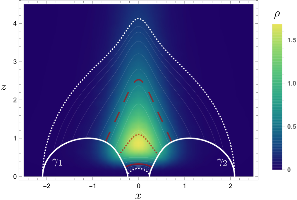
which is everywhere nonnegative and describes a localized dust overdensity, as shown in Fig. 7. Since as or as , the metric approaches AdS at the boundary, as well as away from . The symmetry enforced by ensures that our earlier construction applies. While one could in principle first specify and then determine numerically by solving the differential equation (4), this is a convenient closed-form expression that produces a local blob of dust.
While we know the metric exactly for this dust distribution, we will eschew computing geodesics analytically, since doing so would in this case require solving transcendental, rather than algebraic, equations. However, we can numerically compute geodesic length and construct a wormhole. Let us take and for the boundary-anchored geodesics , as depicted in Fig. 7. We find that by identifying these geodesics, we see that we have indeed engineered a bulge, and we obtain the Python’s Lunch geometry shown in Fig. 8; as in Fig. 5, Fig. 8 is not an embedding diagram, but rather depicts the wormhole width function for this construction as a surface of revolution. The ends of the wormhole flare out as approach the boundary, just as in Fig. 5. However, near the middle of the wormhole, there is a local maximum and two local minima.66 6 A Mathematica notebook that reproduces these numerics is provided as a supplemental file. One can check numerically that , so our entanglement wedge is indeed in the connected phase, with boundary , and that , while , so as required. The various order-one coefficients appearing in Eq. (86) affect properties of the Python’s Lunch such as the size of the bulge in relation to the outer minimal surfaces or the location of the bulge, but our ansatz does not offer us detailed control over these quantities. In particular, one must be careful that the resulting energy density is everywhere positive. Rather, this ansatz is a simple proof of principle for constructing the Python’s Lunch, where the tools (i.e., the large class of -dimensional metrics) to do so in more generality were developed in Sec. 2.

6 Conclusions
The class of metrics constructed in this paper definitively demonstrates that the Python’s Lunch exists in well-defined spacetimes with positive-density matter. It is indeed possible for the minimal surfaces nearest each of the two asymptotic boundaries of a wormhole to not be the same surface, but rather enclose a larger space between them.
More broadly, our class of metrics that we investigated for the step-function dust density exhibits tunable scaling of the entanglement of a boundary subregion, from logarithmic (when ) to volume-law (when ). The broad customizability of this class of geometries, allowing for an arbitrary , provides a multitude of fruitful future directions of study for constructions of interest to holography, including custom-shaped wormholes, deformation of RT surfaces, and behavior reminiscent of black holes.
A potential future direction with respect to the Python’s Lunch geometry is to determine whether the bulge region can be made arbitrarily large. In Ref. [10], geometrical properties of the Python’s Lunch geometry were argued to provide the difference between restricted and unrestricted complexity as argued for by Susskind et al. in Ref. [7] as opposed to that argued by Harlow and Hayden in Ref. [11]. In particular, the maximal cross section of the bulge was in some sense the “intermediate expression swell” of the quantum circuit, while the volume and length approximated the total number of gates and total depth of the circuit, respectively, needed to perform specific operations. It would be interesting if our method of constructing dust geometries—or more general methods—could constrain any of these three parameters, as doing so could bound the degree to which arguments concerning the exponential separation between the two notions of complexity can be encapsulated in a relativistic setting. Another possibility would be to adapt the methods of, e.g., to investigate the phases of bulk reconstructability induced by these bumpy wormhole geometries. We leave these and other avenues to future work.
Acknowledgments
We thank Raphael Bousso, Thomas Hertog, and Don Marolf for useful discussions and comments. N.B. is supported by the National Science Foundation under grant number 82248-13067-44-PHPXH, by the Department of Energy under grant number DE-SC0019380, and by the Computational Science Initiative at Brookhaven National Laboratory. A.C.D. is a Postdoctoral Fellow (Fundamental Research) of the Research Foundation – Flanders (Fonds Wetenschappelijk Onderzoek), File Number 12ZL920N. G.N.R. is supported by the Miller Institute for Basic Research in Science at the University of California, Berkeley.
References
- [1] J. M. Maldacena, “The large- limit of superconformal field theories and supergravity,” Int. J. Theor. Phys. 38 (1999) 1113, arXiv:hep-th/9711200 [hep-th].
- [2] E. Witten, “Anti-de Sitter space and holography,” Adv. Theor. Math. Phys. 2 (1998) 253, arXiv:hep-th/9802150 [hep-th].
- [3] O. Aharony, S. S. Gubser, J. M. Maldacena, H. Ooguri, and Y. Oz, “Large- field theories, string theory and gravity,” Phys. Rept. 323 (2000) 183, arXiv:hep-th/9905111 [hep-th].
- [4] S. Ryu and T. Takayanagi, “Holographic derivation of entanglement entropy from AdS/CFT,” Phys. Rev. Lett. 96 (2006) 181602, arXiv:hep-th/0603001 [hep-th].
- [5] V. E. Hubeny, M. Rangamani, and T. Takayanagi, “A covariant holographic entanglement entropy proposal,” JHEP 07 (2007) 062, arXiv:0705.0016 [hep-th].
- [6] J. Maldacena and L. Susskind, “Cool horizons for entangled black holes,” Fortsch. Phys. 61 (2013) 781, arXiv:1306.0533 [hep-th].
- [7] A. R. Brown, D. A. Roberts, L. Susskind, B. Swingle, and Y. Zhao, “Holographic Complexity Equals Bulk Action?,” Phys. Rev. Lett. 116 (2016) 191301, arXiv:1509.07876 [hep-th].
- [8] A. R. Brown, D. A. Roberts, L. Susskind, B. Swingle, and Y. Zhao, “Complexity, action, and black holes,” Phys. Rev. D93 (2016) 086006, arXiv:1512.04993 [hep-th].
- [9] L. Susskind, “Addendum to Computational Complexity and Black Hole Horizons,” Fortsch. Phys. 64 (2016) 44, arXiv:1403.5695 [hep-th].
- [10] A. R. Brown, H. Gharibyan, G. Penington, and L. Susskind, “The Python’s Lunch: geometric obstructions to decoding Hawking radiation,” arXiv:1912.00228 [hep-th].
- [11] D. Harlow and P. Hayden, “Quantum Computation vs. Firewalls,” JHEP 06 (2013) 085, arXiv:1301.4504 [hep-th].
- [12] D. Marolf, “Black Holes, AdS, and CFTs,” Gen. Rel. Grav. 41 (2009) 903, arXiv:0810.4886 [gr-qc].
- [13] N. Bao, C. Cao, S. M. Carroll, A. Chatwin-Davies, N. Hunter-Jones, J. Pollack, and G. N. Remmen, “Consistency Conditions for an AdS/MERA Correspondence,” Phys. Rev. D91 (2015) 125036, arXiv:1504.06632 [hep-th].
- [14] N. Bao, G. Penington, J. Sorce, and A. C. Wall, “Beyond Toy Models: Distilling Tensor Networks in Full AdS/CFT,” JHEP 11 (2019) 069, arXiv:1812.01171 [hep-th].
- [15] N. Bao, C. Cao, S. Fischetti, and C. Keeler, “Towards Bulk Metric Reconstruction from Extremal Area Variations,” Class. Quant. Grav. 36 (2019) 185002, arXiv:1904.04834 [hep-th].
- [16] F. Pastawski, B. Yoshida, D. Harlow, and J. Preskill, “Holographic quantum error-correcting codes: Toy models for the bulk/boundary correspondence,” JHEP 06 (2015) 149, arXiv:1503.06237 [hep-th].
- [17] T. Takayanagi and K. Umemoto, “Entanglement of purification through holographic duality,” Nature Phys. 14 (2018) 573, arXiv:1708.09393 [hep-th].
- [18] P. Nguyen, T. Devakul, M. G. Halbasch, M. P. Zaletel, and B. Swingle, “Entanglement of purification: from spin chains to holography,” JHEP 01 (2018) 098, arXiv:1709.07424 [hep-th].
- [19] S. Dutta and T. Faulkner, “A canonical purification for the entanglement wedge cross-section,” arXiv:1905.00577 [hep-th].
- [20] N. Bao, A. Chatwin-Davies, J. Pollack, and G. N. Remmen, “Towards a Bit Threads Derivation of Holographic Entanglement of Purification,” JHEP 07 (2019) 152, arXiv:1905.04317 [hep-th].
- [21] Y. Nomura and G. N. Remmen, “Area Law Unification and the Holographic Event Horizon,” JHEP 08 (2018) 063, arXiv:1805.09339 [hep-th].
- [22] R. Bousso, Y. Nomura, and G. N. Remmen, “Outer Entropy and Quasilocal Energy,” Phys. Rev. D99 (2019) 046002, arXiv:1812.06987 [hep-th].
- [23] A. A. García-Díaz, Exact Solutions in Three-Dimensional Gravity. Cambridge Monographs on Mathematical Physics. Cambridge University Press, 2017.
- [24] G. N. Remmen, “New spacetimes for rotating dust in -dimensional general relativity,” Phys. Rev. D 98 (2018) 124008, arXiv:1810.12305 [hep-th].
- [25] D. D. Chow, C. Pope, and E. Sezgin, “Classification of solutions in topologically massive gravity,” Class. Quant. Grav. 27 (2010) 105001, arXiv:0906.3559 [hep-th].
- [26] S. Deser, R. Jackiw, and G. ’t Hooft, “Three-Dimensional Einstein Gravity: Dynamics of Flat Space,” Annals Phys. 152 (1984) 220.
- [27] S. Aminneborg, I. Bengtsson, D. Brill, S. Holst, and P. Peldan, “Black holes and wormholes in (2+1)-dimensions,” Class. Quant. Grav. 15 (1998) 627, arXiv:gr-qc/9707036 [gr-qc].
- [28] D. Brill, “Black holes and wormholes in (2+1)-dimensions,” in Mathematical and Quantum Aspects of Relativity and Cosmology. Proceedings of the Second Samos Meeting on Cosmology, Geometry and Relativity Held at Pythagoreon, Samos, Greece, August 31–September 4, 1998. 1998. arXiv:gr-qc/9904083 [gr-qc].
- [29] N. Engelhardt and A. C. Wall, “Coarse Graining Holographic Black Holes,” JHEP 05 (2019) 160, arXiv:1806.01281 [hep-th].
- [30] B. M. Terhal, M. Horodecki, D. W. Leung, and D. P. DiVincenzo, “The entanglement of purification,” J. Math. Phys. 43 (2002) 4286, arXiv:quant-ph/0202044 [quant-ph].
- [31] N. Bao and N. Cheng, “Multipartite Reflected Entropy,” JHEP 10 (2019) 102, arXiv:1909.03154 [hep-th].
- [32] K. Tamaoka, “Entanglement Wedge Cross Section from the Dual Density Matrix,” Phys. Rev. Lett. 122 (2019) 141601, arXiv:1809.09109 [hep-th].
- [33] J. Kudler-Flam and S. Ryu, “Entanglement negativity and minimal entanglement wedge cross sections in holographic theories,” Phys. Rev. D 99 (2019) 106014, arXiv:1808.00446 [hep-th].
- [34] J. Chu, R. Qi, and Y. Zhou, “Generalizations of Reflected Entropy and the Holographic Dual,” JHEP 03 (2020) 151, arXiv:1909.10456 [hep-th].
- [35] N. Bao and I. F. Halpern, “Conditional and Multipartite Entanglements of Purification and Holography,” Phys. Rev. D99 (2019) 046010, arXiv:1805.00476 [hep-th].
- [36] N. Bao and I. F. Halpern, “Holographic Inequalities and Entanglement of Purification,” JHEP 03 (2018) 006, arXiv:1710.07643 [hep-th].
- [37] K. Umemoto and Y. Zhou, “Entanglement of Purification for Multipartite States and its Holographic Dual,” JHEP 10 (2018) 152, arXiv:1805.02625 [hep-th].
- [38] R. S. K. Mong, K. Siva, B. Swingle, and M. P. Zalatel. In progress.
- [39] R. Bousso and N. Engelhardt, “New area law in general relativity,” Physical Review Letters 115 no. 8, (2015) , arXiv:1504.07627.
- [40] R. Bousso and N. Engelhardt, “Proof of a new area law in general relativity,” Phys. Rev. D 92 no. 4, (2015) 1–14, arXiv:1504.07660.
- [41] S. W. Hawking, “Black holes in general relativity,” Commun. Math. Phys. 25 no. 2, (1972) 152–166.