Uniqueness of STFT phase retrieval for bandlimited functions
Abstract
We consider the problem of phase retrieval from magnitudes of short-time Fourier transform (STFT) measurements. It is well-known that signals are uniquely determined (up to global phase) by their STFT magnitude when the underlying window has an ambiguity function that is nowhere vanishing. It is less clear, however, what can be said in terms of unique phase-retrievability when the ambiguity function of the underlying window vanishes on some of the time-frequency plane. In this short note, we demonstrate that by considering signals in Paley–Wiener spaces, it is possible to prove new uniqueness results for STFT phase retrieval. Among those, we establish a first uniqueness theorem for STFT phase retrieval from magnitude-only samples in a real-valued setting.
1 Introduction
The problem of phase retrieval has been around since the very early days of X-ray crystallography [3, 17]. To date, its applications include coherent diffraction imaging, astronomy and audio processing. The measurements in phase retrieval problems typically consist of phaseless Fourier-type data of the object of interest. Acquisition of magnitude-only measurements means loss of information that needs to be accounted for. One possible approach for phase retrieval is to collect redundant measurements as is done in ptychography for coherent diffraction imaging [5, 13, 16]. There, the idea is that instead of creating one set of measurements through diffraction, a sliding pinhole is added and many masked diffraction patterns are collected. Hence, the measurements can be thought of as magnitudes of windowed Fourier transforms. The same is true for measurements collected in audio processing such as the phase vocoder [9, 15]. Indeed, suppose one wants to alter an audio signal (for instance pitch-shift it). To do so, one can take its short-time Fourier transform (STFT), redistribute the magnitudes thereof in the time-frequency plane and look for a matching audio signal by performing phase retrieval. Motivated by these applications, we consider phaseless measurements of short-time Fourier transforms in this note. More precisely, we analyse the question of unique phase retrievability from STFT magnitudes when the underlying signal is bandlimited.
In general, rather little is known about the uniqueness of phase retrieval from STFT magnitude measurements. A known result is that one may recover signals up to global phase from phaseless STFT measurements when the ambiguity function of the underlying window function is nowhere vanishing [10, 12] (see Lemma 1.2). Additionally, the complement property [1, 2, 4] is a necessary condition for uniqueness. Finally, in the finite-dimensional setting, there is a plethora of results for phase retrieval from discrete short-time Fourier magnitudes [6, 8]. The aim of this note is to provide milder assumptions on the ambiguity function of the window that guarantee uniqueness of STFT phase retrieval when the considered signal class is that of bandlimited functions.
Let us start by summarising relevant prerequisites and fixing notations: For a function , we define the short-time Fourier transform (STFT) (with window function ) by
It can be shown that is uniformly continuous [10]. We consider the phase retrieval problem of recovering from STFT magnitude measurements . Note that it is impossible to distinguish between and , for , from the STFT magnitude measurements alone. For this reason, we aim to reconstruct up to global phase. That is, we attempt to recover the equivalence class
One of the most important properties of the phase retrieval problem with STFT measurements is the ambiguity function relation. We use the convention
for the Fourier transform on and extend it to by a density argument. In addition, we can define the ambiguity function of a signal via
The ambiguity function relation can now be stated as follows:
Lemma 1.1 (Ambiguity function relation).
Let . Then,
We included a proof of this well-known relation in appendix A, for the convenience of the reader. One direct corollary of the ambiguity function relation is that if the ambiguity function of is nowhere vanishing, then one may recover the ambiguity function of everywhere from the STFT magnitude measurements . Furthermore, is uniquely determined up to global phase by its ambiguity function. Combining these observations, one has (see e.g. [10, 12]):
Lemma 1.2.
Let be such that
Then, the following are equivalent for :
- 1.
, for some .
- 2.
.
Clearly, if is such that is zero in some region of , then, using the ambiguity function relation, one cannot recover everywhere. In this note, we ask whether under some additional assumptions, this scenario still enjoys unique phase recovery. In particular, we consider bandlimited functions . It turns out that in this setting it suffices to assume that does not vanish on certain line segments in the time-frequency plane. More precisely, for and , we consider the Paley–Wiener space of bandlimited functions defined as
We record the following classical results on functions in the Paley–Wiener space that we will make use of:
Theorem 1.3 (Paley–Wiener theorem).
Let . Then, the following are equivalent:
- 1.
.
- 2.
is an entire function such that there exists a constant for which
and
Theorem 1.4 (WSK sampling theorem).
Let and . Then, we have
Theorem 1.5 (see Theorem 1 in [18], p. 723).
Let , let and let be real-valued on the real line. Then, can be uniquely determined up to global sign from .
Another property of bandlimited functions that we will employ is that their ambiguity function is compactly supported in frequency domain.
Lemma 1.6.
Let and . Then, is uniformly continuous and .
Proof.
See appendix B. ∎
Therefore, we can consider such that does not vanish on and reconstruct all up to global phase from the STFT magnitude measurements . In what follows, we will show that, in fact, the STFT phase retrieval problem is uniquely solvable for signals in under weaker assumptions on . We remark that our uniqueness results are mainly of theoretical interest and do not suggest a method for stable phase recovery.
Outline
This paper is divided into two main parts. First, in Section 2, we consider signals in the Paley–Wiener space which are real-valued on the real line and develop two uniqueness results for this case: In particular, we show that if the ambiguity function of the window is non-zero almost everywhere on a certain line segment in the time-frequency plane, then all bandlimited signals are uniquely determined by their STFT magnitudes (Subsection 2.1). In addition, we show that if the Fourier transform of the window is non-zero almost everywhere on an open interval around the origin and if the window is real-valued itself, then all bandlimited signals are uniquely determined by samples of their STFT magnitudes (Subsection 2.2). Secondly, in Section 3, we consider general signals in the Paley–Wiener space and develop two uniqueness results in this setting. More precisely, we show that if the ambiguity function of the window is non-zero almost everywhere on two parallel line segments in the time-frequency plane that are sufficiently close together, then uniqueness of phase retrieval from STFT magnitudes holds for all signals in (Subsection 3.1). In addition, we show that if the ambiguity function of the window does not vanish on a single line segment in the time-frequency plane, then all bandlimited signals are uniquely determined by their STFT magnitudes (Subsection 3.2). In Section 4, we discuss our results for some examples of window classes.
2 Real-valued signals
2.1 Reconstruction from full measurements
If , for some , and the window is such that , for , then one can use the Ambiguity Function Relation to obtain everywhere. Therefore, one can recover on the real line via Fourier inversion. If is real-valued on the real line, this is enough to recover everywhere up to global phase [18] (see Theorem 1.5). The last insight is particularly important such that we state it as a lemma.
Lemma 2.1.
Let and be real-valued on the real line. Then, is uniquely determined by up to global sign.
Proof.
This follows immediately from Theorem 1.5. Alternatively, one might consider the following argument: Let us assume without loss of generality that is non-trivial. By the Paley–Wiener theorem (see Theorem 1.3), is an entire function. The roots of a non-zero entire function are isolated and therefore there must exist an interval such that for all , . Therefore, agrees with up to global sign on . In other words, is the restriction of or to the interval and thus analytically extending from to yields or . ∎
Note that the same does not hold for general signals. Indeed, consider the following counterexample.
Example 2.2.
Let , and , for . One can readily show that
Therefore, we have . In addition,
but and do not agree up to global phase.
Many more counterexamples may be constructed using Hadamard’s factorisation theorem and ideas similar to the ones in [14]. We may now combine the lemma above with the ambiguity function relation to derive the following theorem.
Theorem 2.3.
Let and such that
Then, the following are equivalent for real-valued on the real line:
- 1.
.
- 2.
.
Proof.
First, note that if , then it follows immediately that . Secondly, suppose that . It follows from the ambiguity function relation that
Hence, by the assumption on the ambiguity function of the window, , for a.e. . By the Paley–Wiener theorem, and are square integrable and thus and are (uniformly) continuous. Therefore, , for all . We know from Lemma 1.6 that and consequently, that . Since
we have . Applying Lemma 2.1 yields the assertion. ∎
Remark 2.4.
Using basic Fourier-analytic results, one can show a statement which is similar to Theorem 2.3 for compactly supported, even, real-valued functions:
Let and such that
Then, the following are equivalent for even and real-valued:
- 1.
.
- 2.
.
2.2 Reconstruction from sampled STFT measurements
So far, we have not used the sampling theorem in [18] for the reconstruction from samples of the STFT magnitudes. Let us consider the same setup as before and ask whether the phase is uniquely determined by sampled data. To the best of our knowledge, the following is the first uniqueness result for phase retrieval from sampled STFT magnitude measurements.
Theorem 2.5.
Let and let be a real-valued window such that
Then, the following are equivalent for real-valued on the real line:
- 1.
.
- 2.
, for all .
Proof.
First, note that if , then it follows immediately that
Secondly, assume that the above equation holds. Let us define , for (this simplifies to because is real-valued). Note that
and hence
As , it follows from the convolution theorem that and extend to functions in . Indeed, as , there exists such that
Now, consider . Then, by the convolution theorem,
Therefore, the analytic extensions of and belong to . In addition, and are real-valued such that it follows from Theorem 1.5 that . Consequently, we have
By the assumption on the Fourier transform of the window, it follows that and hence, . ∎
Remark 2.6.
We observe the following:
- 1.
The sampling rate only depends on the bandwidth of the signals and is exactly twice the Nyquist rate.
- 2.
For the Gaussian , , we can readily see that is non-zero everywhere. In addition, the Gaussian is real-valued such that the theorem above implies that all bandlimited signals are uniquely determined by samples of their STFT magnitudes with Gaussian window (also called Gabor transform magnitudes).
- 3.
We use the uniform sampling sequence , for convenience of notation. In fact, our result still holds if one replaces by any separated, uniformly dense sampling sequence with density lower bounded by [18].
- 4.
While the STFT is complex-valued, we employ only real-valued information on one line of the time-frequency plane. On this line, sign retrieval suffices for the uniqueness result to hold.
3 Complex-valued signals
3.1 Using the ambiguity function on two line segments
We have seen that for complex-valued , it is not true that is uniquely determined up to global phase by . Therefore, we need to change our strategy to deduce a general uniqueness result. One can, for instance, impose slightly stronger assumptions on the ambiguity function of the window to show that in this case one may recover uniquely up to global phase from .
Theorem 3.1.
Let , and such that
for a.e. . Then, the following are equivalent for :
- 1.
, for some .
- 2.
.
Proof.
First, note that if , for some , then it follows immediately that . Secondly, suppose that . Let us also assume without loss of generality that and are non-zero. As in the proof of Theorem 2.3, we find that and . Therefore, on and
By the Paley–Wiener theorem, and are entire functions. Therefore, we know that and have a countable number of roots (as their roots are isolated). In particular, there exists some such that for all , we have
Now, let us set to be such that
Then, we can use the relation
to recursively find that
Finally, since and , it follows that . Therefore, we deduce from the WSK sampling theorem (see Theorem 1.4) that
for all . Hence, we conclude that . ∎
Remark 3.2.
We can apply basic Fourier analysis to develop a result similar to Theorem 3.1 for compactly supported functions:
Let , and such that
for a.e. . Then, the following are equivalent for :
- 1.
, for some .
- 2.
.
We note that the requirement is linked to the use of the WSK sampling theorem in the proof of the above result. The following example shows that it is necessary in order for to be uniquely determined up to global phase by and , for .
Example 3.3.
Let and . Consider as well as , for . Then, it is readily seen that
as well as
Therefore, we have . In addition,
as well as
hold, for . However, and do not agree up to global phase.
Many more examples may be constructed using Hadamard’s factorisation theorem and ideas similar to the ones in [14].
3.2 Using the ambiguity function on a single line segment
We can approach the reconstruction of general bandlimited functions from their STFT magnitude measurements from a slightly different angle and obtain another uniqueness result. The following statement is neither stronger nor weaker than Theorem 3.1: Indeed, it has the advantage that one only needs to assume that the ambiguity function of the window does not vanish on a single line segment while having the disadvantage that one has to make this assumption pointwise and not in an -sense.
Theorem 3.4.
Let and be such that
Then, the following are equivalent for :
- 1.
, for some .
- 2.
.
Proof.
First, note that if , for some , then it follows immediately that . Secondly, suppose that and assume without loss of generality that and are non-zero. Note that is continuous such that is continuous and by assumption , for . By the extreme value theorem, there exists a positive constant such that , for . As is uniformly continuous, there exists a such that
In particular, it follows that
Lemma 1.1 further implies
Hence, by employing Lemma 1.6, we deduce that , for . By Fourier inversion, we have
for . As and are entire functions and assumed to be non-zero, there exists a such that . As , it follows that there exists an such that . This implies that for all . As and are entire, we conclude that . ∎
Remark 3.5.
As before, we can make a similar statement as the above for compactly supported functions:
Let and be such that
Then, the following are equivalent for :
- 1.
, for some .
- 2.
.
4 Examples
In the following, we want to consider different windows and their ambiguity functions in order to put the results which we have developed in context. We start by considering the most well-known window in time-frequency analysis: The Gaussian window , for (see Figure 1). For the Gaussian, one can show that


Therefore, is nowhere vanishing and all may be uniquely recovered up to global phase from their STFT magnitude measurements . Note that this already follows from the classical theory about uniqueness of STFT phase retrieval (Lemma 1.2). One could be tempted to believe that the only windows for which the ambiguity functions are non-zero everywhere are the generalised Gaussians , where is a polynomial of degree two. This belief is wrong, however, as was recently shown in [11], and one can in fact construct more functions such that everywhere. Finally, note that is real-valued and that the Fourier transform of is also a Gaussian. In particular, vanishes nowhere and it follows from Theorem 2.5 that for all , one can recover all that are real-valued on the real line up to global sign from the sampled measurements , for .
The next class of window functions we want to study is that of the Hermite functions. We define the monomials
for . One can show that these monomials form an orthonormal basis of the Fock space [10]. The pre-images of these monomials under the Bargmann transform are called Hermite functions and we write , for . The ambiguity function of the Hermite functions can be expressed in terms of the Laguerre polynomials
where [7]. In particular, we have for all and that (see Figure 2 and Figure 3 for an illustration):


Therefore, the set of roots of consists of concentric rings around the origin of the time-frequency plane. The radius of these rings is determined by the positive roots of the -th Laguerre polynomial . In particular, is non-zero almost everywhere and it follows from Lemma 1.2 that all are uniquely determined up to global phase by their STFT measurements. As for the Gaussian case, uniqueness of STFT phase retrieval already follows from the ambiguity function relation. Note that the Fourier transform of the Hermite function is [10]. In addition, one can show that , , is a polynomial of degree [7]. It follows that has only finitely many roots and thus is non-zero almost everywhere. In addition, as is real-valued, it follows from Theorem 2.5 that for all , it holds that all that are real-valued on the real line can be recovered up to global sign from the sampled measurements , for .
The third class of window functions, we consider is that of compactly supported window functions. This class includes all windows commonly used in practice. Consider for instance the rectangular window
or the Hanning window . If is compactly supported, then for any fixed , the function is bandlimited. In particular, extends to an analytic function on the complex plane. Therefore, is either zero or has merely isolated zeroes on the real line. Hence, we can conclude that for all such that is not the trivial map, it holds that
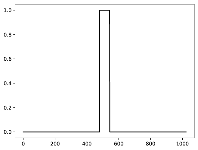


For a depiction of the ambiguity functions of the rectangular and Hanning windows see Figure 4 and Figure 5, respectively. As , it follows that for a.e. , as long as is not the trivial window. Therefore, Theorem 2.3 implies that for all , it holds that all which are real-valued on the real line are uniquely determined up to global sign by their STFT measurements. We can say more, however. If is not the trivial window, then . As is continuous, it follows that for all which are small enough, . Therefore, for almost every . By Theorem 3.1, we find that for all , it holds that all are uniquely determined up to global phase by their STFT magnitudes.
Acknowledgements
The authors would like to thank Giovanni S. Alberti for fruitful discussions and acknowledge funding through SNF Grant 200021_184698.
Appendix A The ambiguity function relation
Proof of the ambiguity function relation.
Using the family given by
for , allows us to write
In addition, we can readily see that
where , for . Let be fixed but arbitrary. As , it follows from the convolution theorem that
As (by the orthogonality relations of the STFT [10]), it follows that the STFT magnitude measurements squared are in and thus the Fourier inversion theorem implies that
for . Finally, we can see the above as a function in and note that
for , by the triangle inequality, Tonelli’s theorem, a change of variables and Cauchy–Schwarz. Therefore, we may take the Fourier transform in and obtain
for , by Fubini’s theorem and a change of variables. Finally, note that all the equalities in this proof are actual equalities as all functions that we compare are continuous functions by virtue of them being Fourier transforms of functions. ∎
Appendix B The ambiguity function of a Paley–Wiener function
Proof of Lemma 1.6.
It follows from Plancherel’s theorem that the restriction of to the real line is in . Therefore, is uniformly continuous [10]. Now, define , for , and let be arbitrary but fixed. We compute
using the convolution theorem. Furthermore, we find that
Therefore, we have
If is such that , then we can readily see that , for . It follows that . ∎
References
- [1] Balan, R., Casazza, P. G., & Edidin, D. (2006). On signal reconstruction without phase. Applied and Computational Harmonic Analysis, 20(3), 345–356. https://doi.org/10.1016/j.acha.2005.07.001
- [2] Bandeira, A. S., Cahill, J., Mixon, D. G., & Nelson, A. A. (2014). Saving phase: Injectivity and stability for phase retrieval. Applied and Computational Harmonic Analysis, 37(1), 106–125. https://doi.org/10.1016/j.acha.2013.10.002
- [3] Bragg, L. (1960). The Rutherford memorial lecture, 1960. The development of X-ray analysis. Proceedings of the Royal Society of London. Series A, Mathematical and Physical Sciences, 262(1309), 145–158. Retrieved May 29, 2020, from www.jstor.org/stable/2414072
- [4] Cahill, J., Casazza, P. G., & Daubechies, I. (2016). Phase retrieval in infinite-dimensional Hilbert spaces. Transactions of the American Mathematical Society, Series B, 3(3), 63–76. https://doi.org/10.1090/btran/12
- [5] Chapman, H. N. (1996). Phase retrieval X-ray microscopy by Wigner-distribution deconvolution. Ultramicroscopy, 66(3–4), 153–172. https://doi.org/10.1016/S0304-3991(96)00084-8
- [6] Eldar, Y. C., Sidorenko, P., Mixon, D. G., Barel, S., & Cohen, O. (2014). Sparse phase retrieval from short-time Fourier measurements. IEEE Signal Processing Letters, 22(5), 638–642. https://doi.org/10.1109/LSP.2014.2364225
- [7] Folland, G. B. (1989). Harmonic Analysis in Phase Space. (AM-122) (1st ed.). Princeton University Press.
- [8] Pfander, G. E., & Zheltov, P. (2015). Estimation of overspread scattering functions. IEEE Transactions on Signal Processing, 63(10), 2451–2463. https://doi.org/10.1109/TSP.2015.2403309
- [9] Griffin, D. W., & Lim, J. S. (1984). Signal estimation from modified short-time Fourier transform. IEEE Transactions on Acoustics, Speech, and Signal Processing, 32(2), 236–243. https://doi.org/10.1109/TASSP.1984.1164317
- [10] Gröchenig, K. (2001). Foundations of time-frequency analysis (1st ed.). Birkhäuser.
- [11] Gröchenig, K., Jaming, P., & Malinnikova, E. (2019). Zeros of the Wigner distribution and the short-time Fourier transform. Revista Matemàtica Complutense. Advance online publication. https://doi.org/10.1007/s13163-019-00335-w
- [12] Grohs, P., & Rathmair, M. (2018). Stable Gabor phase retrieval and spectral clustering. Communications On Pure And Applied Mathematics, 72(5), 981-1043. https://doi.org/10.1002/cpa.21799
- [13] Hegerl, R., & Hoppe, W. (1970). Dynamische Theorie der Kristallstrukturanalyse durch Elektronenbeugung im inhomogenen Primärstrahlwellenfeld. Berichte der Bunsengesellschaft für physikalische Chemie, 74(11), 1148–1154. https://doi.org/10.1002/bbpc.19700741112
- [14] Mc Donald, J. N. (2004). Phase retrieval and magnitude retrieval of entire functions. Journal of Fourier Analysis and Applications, 10(3), 259–267. https://doi.org/10.1007/s00041-004-0973-9
- [15] Průša, Z., Balazs, P., & Søndergaard, P. L. (2017). A noniterative method for reconstruction of phase from STFT magnitude. IEEE/ACM Transactions on Audio, Speech, and Language Processing, 25(5), 1154–1164. https://doi.org/10.1109/TASLP.2017.2678166
- [16] Rodenburg, J. M. (2008). Ptychography and related diffractive imaging methods. Advances in Imaging and Electron Physics, 150, 87–184. https://doi.org/10.1016/S1076-5670(07)00003-1
- [17] Sayre, D. (2002). X-ray chrystallography: The past and present of the phase problem. Structural Chemistry, 13, 81–96. https://doi.org/10.1023/A:1013477415486
- [18] Thakur, G. (2010). Reconstruction of bandlimited functions from unsigned samples. Journal Of Fourier Analysis And Applications, 17(4), 720-732. https://doi.org/10.1007/s00041-010-9144-3