Microscopic Calculation of Folding Potential
Abstract
We construct a folding potential between the and particles based on underlying nucleon-nucleon and hyperon-nucleon interactions. Starting from a phenomenological -N potential and a Gaussian form of the -particle wave function we obtain for the built - interaction a bound He state with the binding energy (3.10 MeV), which is consistent with recent experimental data MeV. When in turn an exact solution of the four-body Faddeev-Yakubovsky equation for the -particle calculated with the CDBonn, Nijmegen or Argonne V18 realistic nucleon-nucleon potential is used and the phenomenological Gaussian -N potential is replaced by the realistic (Nijmegen NSC97f) potential approximated by a rank-1 separable form, then He is overbound. In particular, its binding energy given by the folding potential generated with the particle wave function based on the CDBonn potential is 7.47 MeV. Although the rank-1 separable -N potential reproduces the exact scattering length and the effective range of the original -N potential, the overbinding results from the lack of the required repulsive properties in the assumed separable form.
pacs
21.45.-v,21.60.Gx,21.80.+aI Introduction
The strangeness sector of few-body systems still poses many problems despite many years of strong efforts[1]. Hyperon-nucleon (YN) and hyperon-hyperon (YY) forces are to a large extent unknown due to the sparsity of direct YN or indirect YY data. Thus the situation is quite different from the nucleon-nucleon (NN) case, where thousands of available data points strongly constrain the spin-momentum dependencies of nucleon-nucleon force models. In the case of -N or -N (strangeness S=-1 sector) the set of scattering data is very small [2] and is not sufficient to determine well the properties of those forces. On the theoretical side one is still far away from a solution of the underlying theory of the strong interaction, QCD, and therefore effective approaches are used to generate forces. They are either based on meson exchanges, like the ones by the Nijmegen [3], Jülich[4], or Ehime[5] groups, or on quark models, like the ones by the Kyoto-Niigata [6], the Tokyo[7], the Salamanca [8] or the Beijing[9] groups. Despite all this work, there remains a lot of uncertainty about the properties of the baryon-baryon forces, especially in the strangeness S=-2 sector.
Beside the above-mentioned potentials, there exist also modified versions of the realistic Nijmegen potential, widely used in [10], which are phase equivalent to the original ones and are parameterized in the Gaussian form. These YN and YY interactions constitute the dynamical input for few-body equations, whose solutions lead to observables, which can be compared to experimental data. The lightest hypernuclei H, H and He with strangeness S=-1 have been studied extensively, by evaluating their binding energies and lowest excitation energies by employing various potential models. The results are still ambiguous. The binding energy of the lightest hypernucleus H can be satisfactorily reproduced using directly some of the Nijmegen forces [11].
However, when the Nijmegen YN forces NSC89 [18] and NSC97a-f NSC97f are employed, no adequate description of H and He is achieved [12], whereas more phenomenological forces come closer to the data[13]. Phenomenological central -N potentials overbind He, which is well known for its anomalously small binding energy. This problem seems to be solved by a recent variational 5-body calculation[13] using forces stemming from the original Nijmegen ones.
Certain heavier hypernuclei can also be viewed as few-body systems assuming their cluster structure in terms of the -particles. Phenomenological potentials of a simple Gaussian type were used e.g. to study double- hypernuclei [14]. Recently, we predicted the existence of quasi-bound state of the system employing a phenomenological potential [15]. The common drawback of all phenomenological potentials is that they have some parameters to be fit to experimental data. In order to obtain a potential without any unknown parameters, one has to solve a N-body problem driven by baryon-baryon interactions which is, however, very difficult beyond the four-body system.
In this paper we derive a folding potential between the and particles without any additional parameters. Our paper is organized as follows. In the next section we explain how to introduce the folding potential in question. In order to achieve this goal we use the -particle wave function based on realistic NN forces, e.g., a meson theoretical CD-Bonn [16], Nijmegen Nijm93 and Argonne AV18 potentials and we describe the -N interaction by a phenomenological Gaussian form [19] and meson theoretical models, e. g., Chiral chiral, Jülich Juelich, Nijmegen NSC97f; ND and EhimeEhime. In order to facilitate calculations, these meson theoretical -N potentials are modified into convenient separable approximations. In Sec. III we calculate binding energies of He employing many versions of the folding potential. Finally, in Sec. IV we discuss and summarize these results.
II Method of Calculation
The construction of the folding potential is performed by using the -particle wave function from the solution of the Faddeev-Yakubovsky equations based on realistic NN forces. The -N interaction is first taken in the form of a phenomenological Gaussian potential [19]. Later we will replace the Gaussian potential by a more realistic one. The folding potential is defined by evaluating matrix elements of the inner realistic potential between products of two-cluster wave functions :
| (1) |
The schematic diagram of the potential is shown in Fig. 1. For the case at hand, the wave functions and correspond to the and particles. The -particle wave function is obtained by solving the Faddeev-Yakubovsky equations [20] in momentum space in the partial wave basis. The natural Jacobi momenta for the partition [20] are
| (2) | |||
| (3) |
| (4) |
where are the individual nucleon momenta, is the momentum of the hyperon; and are the masses of the nucleon and the particle.


The corresponding relative orbital angular momenta will be denoted by and the total spin, total angular momenta and total isospins in the various subsystems by and , respectively (see Fig. 2). The 4N- basis states are introduced via
| (5) | |||
| (6) |
where the brackets indicate self-explanatory consecutive couplings to the total five-baryon angular momentum and total isospin with the corresponding magnetic quantum numbers (not shown for brevity). The quantum numbers for channels and are listed in Tab. 1. The natural Jacobi momenta for the fragmentation are
| (7) | |||
| (8) |
The corresponding discrete quantum numbers will be denoted by Greek letters, see the right panel of Fig. 2. The basis states are
| (9) | |||
| (10) |
where the brackets indicate again the sequences of couplings of angular momenta and isospins. The Jacobi momenta in these two sets are related via
| (11) |
In order to calculate the folding potential of Eq. (1) we first prepare the -particle wave function and the YN interaction as
| (12) | |||
| (13) |
Then Eq.(1) turns into
| (14) | |||
| (15) | |||
| (16) |
where
| (17) |
and is taken is as a plane wave. The geometrical functions and have been introduced in Refs. GloeckleTEXT; Gloeckle1996 and for the sake of the reader are displayed in Appendix A.
| 1 | 0 | 0 | 0 | 1/2 | 0 | 1/2 | 0 | 0 | 0 | 0 | 1/2 |
| 2 | 0 | 1 | 1 | 1/2 | 0 | 1/2 | 0 | 0 | 0 | 0 | 1/2 |
| 3 | 2 | 1 | 1 | 1/2 | 0 | 1/2 | 0 | 0 | 0 | 0 | 1/2 |
| 4 | 0 | 1 | 1 | 3/2 | 2 | 1/2 | 0 | 0 | 0 | 0 | 1/2 |
| 5 | 2 | 1 | 1 | 3/2 | 2 | 1/2 | 0 | 0 | 0 | 0 | 1/2 |
| 1 | 0 | 0 | 0 | 1/2 | 0 | 1/2 | 0 | 0 | 0 | 0 | 1/2 |
| 2 | 0 | 1 | 1 | 1/2 | 0 | 1/2 | 0 | 0 | 0 | 0 | 1/2 |
| 3 | 2 | 1 | 1 | 1/2 | 0 | 1/2 | 0 | 0 | 0 | 0 | 1/2 |
| 4 | 0 | 1 | 1 | 3/2 | 2 | 1/2 | 0 | 0 | 0 | 0 | 1/2 |
| 5 | 2 | 1 | 1 | 3/2 | 2 | 1/2 | 0 | 0 | 0 | 0 | 1/2 |
| 6 | 0 | 0 | 0 | 1/2 | 0 | 1/2 | 0 | 1 | 1 | 0 | 1/2 |
| 7 | 0 | 1 | 1 | 1/2 | 0 | 1/2 | 0 | 1 | 1 | 0 | 1/2 |
| 8 | 2 | 1 | 1 | 1/2 | 0 | 1/2 | 0 | 1 | 1 | 0 | 1/2 |
| 9 | 0 | 1 | 1 | 3/2 | 2 | 1/2 | 0 | 1 | 1 | 0 | 1/2 |
| 10 | 2 | 1 | 1 | 3/2 | 2 | 1/2 | 0 | 1 | 1 | 0 | 1/2 |
| 11 | 0 | 0 | 0 | 1/2 | 0 | 1/2 | 2 | 1 | 1 | 0 | 1/2 |
| 12 | 0 | 1 | 1 | 1/2 | 0 | 1/2 | 2 | 1 | 1 | 0 | 1/2 |
| 13 | 2 | 1 | 1 | 1/2 | 0 | 1/2 | 2 | 1 | 1 | 0 | 1/2 |
| 14 | 0 | 1 | 1 | 3/2 | 2 | 1/2 | 2 | 1 | 1 | 0 | 1/2 |
| 15 | 2 | 1 | 1 | 3/2 | 2 | 1/2 | 2 | 1 | 1 | 0 | 1/2 |
III Numerical results
First let us consider results for the potential obtained with some phenomenological -N force. There are many phenomenological models of the -N interaction, e.g., a hard-core one represented by exponential functions [21]; [22]; [23] or a multi-Gaussian type [24]; Hiyama1997 inspired by the YNG Potential [25]:
| (18) |
The spin-dependent phenomenological -N interaction is parameterized by Hiyama et al.,[19] as
| (19) |
with -38.19MeV, =1.034 fm and =-0.1. The -N potential for the spin triplet is shown in Fig. 3 and the quantum numbers for channels and are listed in Tab. I for the total and the total isospin T=0, assuming the positive parity and restricting to =0, = 2, = 1. The phenomenological potentials of Eqs. (3.1)–(3.2) are often converted into the potential with the use of the Resonating Group Method (RGM) Technique [14]; [26]; Hiyama1997, which is based on the shell-model Gaussian wave function. Specifically, the integral kernel of Eq. (17) originating from the Gaussian particle S-wave function is given as
| (20) |
where the width parameter is a common shell model mode [14]; [26] taken to be 0.275 fm-2.
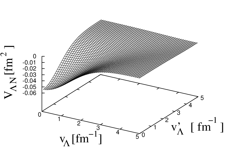
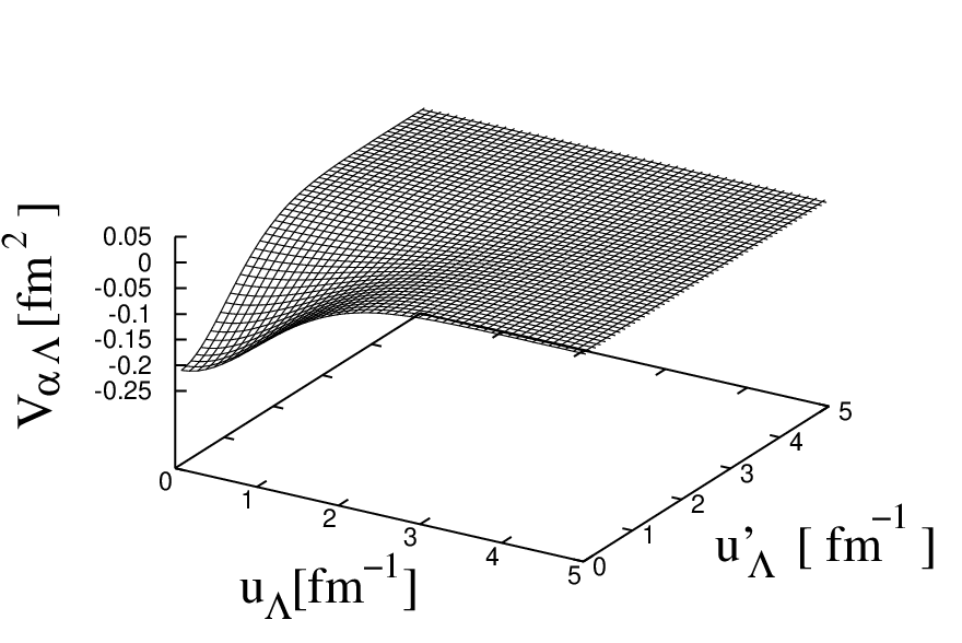
We obtained a - folding potential (shown in Fig.4) for which the He binding energy is -3.10 MeV. The calculated binding energy compares well with the data (-3.12 0.02 MeV) Gal1975. This consistence is to be expected, since the YN potential of Eq. (19) is adjusted to the experimental He binding energy when the RGM technique is employed.
Next we replace the simple Gaussian wave function of the particle by the wave function based on the realistic NN forces: the CD-Bonn[16], Nijmegen Nijm93, and Argonne V18 AV18 potentials. Our experience with the particle wave functions obtained with these potentials indicates that the S-wave contribution is essential to provide the correct binding energy. Thus in the following calculations we could restrict ourselves to only few partial waves and solve the Faddeev-Yakubovsky equation for the particle in the basis comprising and states.
On the other hand, the -N potentials are given in the separable form:
| (21) |
where and are the coupling constant and the form factor, respectively. In order to check the accuracy of the separable approximation we prepare two kinds of the separable potentials, e.g, the Yamaguchi type (Y) and the Gaussian type (G). The form factors of these potential are given as
| (22) | |||
| (23) |
The meson theoretical -N potentials are constructed to describe the -N scattering data. However, due to the sparsity of the data parameters of all potential models are not well determined. Therefore, we use the fact that the -N scattering amplitude in the low energy limit can be determined from the well-known effective range expansion which has the form
| (24) |
where denotes the scattering momentum in the center-of-mass system and the parameters [fm] and [fm] are often called the scattering length and the effective range, respectively. The phase shift of each partial wave is linked to the scattering amplitude.
These effective range expansion parameters are directly connected to the quantities , , and from Eq. (23) by the following relations.
| (25) | |||
| (26) | |||
| (27) | |||
| (28) |
where is the reduced mass of the -N system. In the case of the Yamaguchi type form factors these relations are proved in Ref. afnan2015. Tables 2 and 3 collect the scattering lengths and the effective ranges from several -N potentials. Choosing only the and partial waves of the N potential we can substantially simplify the folding potential from the complicated form given in Eq. (16) and arrive at
| (29) | |||
| (30) |
One can note that the spin-spin dependence of the Hiyama N potential of Eq. (19) disappears due to the weighted ( and ) sum in Eq. (30).
| Model N potential | a () | r () | a () | r () |
|---|---|---|---|---|
| Hiyama et al. [19] | -1.28* | 2.33* | -0.67* | 3.08* |
| Chiral ( = 600) chiral; afnan2015 | -2.91* | 2.78* | -1.54* | 2.74* |
| Jülich04 Juelich; afnan2015 | -2.56* | 2.75* | -1.66* | 2.93* |
| Nimegen ESC16 | -1.96 | 3.65 | -1.84 | 3.33 |
| Nijmegen NSC97e NSC97f; afnan2015 | -2.24 | 3.24 | -1.83 | 3.14 |
| Nijmegen NSC97f NSC97f; afnan2015 | -2.68 | 3.07 | -1.67 | 3.34 |
| Nijmegen NSC89 [18] | -2.86 | 2.91 | -1.24 | 3.33 |
| Nimegen HC-D model ND; afnan2015 | -2.03 | 3.66 | -1.84 | 3.32 |
| Ehime set 2 Ehime | -2.65* | 3.24* | -1.80* | 3.71* |
| Ehime set A Ehime | -2.76* | 3.19* | -2.064* | 3.46* |
| Ehime set B Ehime | -2.71* | 3.21* | -1.95* | 3.56* |
| Model N potential | a () | r () | a () | r () |
|---|---|---|---|---|
| Nimegen ESC16 | -1.88 | 3.58 | -1.86 | 3.37 |
| Nijmegen NSC97e NSC97f; afnan2015 | -2.10 | 3.19 | -1.86 | 3.19 |
| Nijmegen NSC97f NSC97f; afnan2015 | -2.51 | 3.03 | -1.75 | 3.32 |
| Nijmegen NSC89 [18] | -2.73 | 2.87 | -1.48 | 3.04 |
| Nimegen HC-D model ND; afnan2015 | -2.06 | 3.78 | -1.77 | 3.18 |
|
|
|
|
|
| |||||||||||||
|---|---|---|---|---|---|---|---|---|---|---|---|---|---|---|---|---|---|---|
| Hiyama et al. [19] | -3.10 | -2.99 | -2.18 | -2.54 | -1.98 | -1.95 | ||||||||||||
| Hiyama (Y) | -2.46 | -2.36 | -1.62 | -1.94 | -1.44 | -1.42 | ||||||||||||
| Hiyama (G) | -3.07 | -2.89 | -2.12 | -2.46 | -1.92 | -1.90 | ||||||||||||
| Chiral ( = 600) chiral; afnan2015 (Y) | -8.44 | -8.26 | -6.64 | -7.36 | -6.21 | -6.16 | ||||||||||||
| Chiral ( = 600) (G) | -9.26 | -8.83 | -7.42 | -8.08 | -7.03 | -6.99 | ||||||||||||
| Jülich04 Juelich; afnan2015 (Y) | -8.47 | -8.26 | -6.68 | -7.39 | -6.26 | -6.21 | ||||||||||||
| Jülich04 (G) | -9.08 | -8.62 | -7.29 | -7.92 | -6.93 | -6.89 | ||||||||||||
| Nimegen ESC16 (Y) | -7.57 | -7.27 | -5.98 | -6.57 | -5.65 | -5.61 | ||||||||||||
| Nimegen ESC16 (G) | -7.38 | -6.85 | -5.93 | -6.39 | -5.68 | -5.67 | ||||||||||||
| Nijmegen NSC97e NSC97f; afnan2015 (Y) | -8.22 | -7.94 | -6.51 | -7.16 | -6.13 | -6.09 | ||||||||||||
| Nijmegen NSC97e (G) | -8.32 | -7.80 | -6.71 | -7.24 | -6.41 | -6.39 | ||||||||||||
| Nijmegen NSC97f NSC97f; afnan2015 (Y) | -7.98 | -7.70 | -6.32 | -6.95 | -5.95 | -5.91 | ||||||||||||
| Nijmegen NSC97f (G) | -8.00 | -7.47 | -6.44 | -6.95 | -6.16 | -6.14 | ||||||||||||
| Nijmegen NSC89 [18] (Y) | -7.12 | -6.88 | -5.54 | -6.15 | -5.19 | -5.15 | ||||||||||||
| Nijmegen NSC89 (G) | -7.48 | -7.03 | -5.93 | -6.46 | -5.64 | -5.61 | ||||||||||||
| Nimegen HC-D model ND; afnan2015 (Y) | -7.62 | -7.32 | -6.02 | -6.62 | -5.68 | -5.64 | ||||||||||||
| Nimegen HC-D model (G) | -7.48 | -6.96 | -6.01 | -6.48 | -5.75 | -5.74 | ||||||||||||
| Ehime set 2 Ehime (Y) | -7.65 | -7.32 | -6.08 | -6.66 | -5.76 | -5.73 | ||||||||||||
| Ehime set 2 Ehime (G) | -7.22 | -6.66 | -5.83 | -625 | -5.60 | -5.60 | ||||||||||||
| Ehime set A Ehime (Y) | -8.79 | -8.45 | -7.05 | -7.70 | -6.68 | -6.64 | ||||||||||||
| Ehime set A Ehime (G) | -8.45 | -7.85 | -6.89 | -7.37 | -6.62 | -6.61 | ||||||||||||
| Ehime set B Ehime (Y) | -8.31 | -7.97 | -6.64 | -7.26 | -6.29 | -6.26 | ||||||||||||
| Ehime set B Ehime (G) | -7.93 | -7.35 | -6.44 | -6.90 | -6.19 | -6.18 |
In Tab. 4 we demonstrate the calculated binding energies of the He hypernucleus. Each row of the table is prepared for one -N potential. The row containing results based on the full potential from Hiyama et al.[19]) is separated from the other ones by a line to indicate that the predictions in all other rows are obtained with separable approximations employing the Yamaguchi type (Y) or the Gaussian type (G) form factors. Columns tell which realistic NN potential is used to calculate the particle wave function, necessary to construct the integral kernel in Eq.(17) or in Eq. (20). The column denoted as RGM Hiyama1997 is an exception because here the particle wave function has a simple Gaussian form, with fm-2.
From the comparison of the binding energies for the Gaussian wave function with the full Hiyama Gaussian N potential (-3.10 MeV), the approximate Hiyama potential (type Y) (-2.46 MeV) and the approximate Hiyama potential (type G) (3.07 MeV), we can estimate the accuracy of the separable approximation. The accuracy is not better than approximately 0.7 MeV. Using the realistic particle wave functions we obtain clear underbinding. It is most evident for the AV18 potential and predictions based on this NN force differ from the others by up to 1.2 MeV.
Surprisingly, the most realistic input for calculations, namely the realistic -N potential and the particle wave functions generated by the realistic NN interactions, leads to rather strong overbinding of the He hypernucleus and moves the predictions away from the data. These numbers are listed below the second horizontal line in Tab. 4.
IV Summary and Outlook
We have prepared many versions of the - folding potential which required both particle wave functions and -N potentials. To this end we considered not only the simple Gaussian form of the particle wave function but also wave functions generated as rigorous solutions of the four-nucleon Faddeev-Yakubovsky equation with several realistic NN potentials. For the -N potential we have taken the full and approximated phenomenological Hiyama model Hiyama1997 but also the meson theoretical ones. In order to facilitate our calculations we prepared and utilized simplified separable versions of the -N realistic potentials, taking care to realize exactly their crucial features, the scattering length and the effective range.
First we employed the Hiyama phenomenological -N potential together with the Gaussian particle wave function and obtained the binding energy of He -3.10 MeV, which is in agreement with the experimental data (-3.12 0.02 MeV).
All the N potentials used in this paper reproduce both the scattering length and the effective range in the and states. These features are shown in Tabs. 2 and 3. Because there is no possibility to compare these parameters with the data, these numbers are to some extent arbitrary. Preserving these features rank-1 separable potentials are prepared as given in Eqs. (21)–(28). The separable approximation of the Gaussian type reproduces very well the prediction based on the original phenomenological potential, yielding the binding energy -3.07 MeV, which is very close to the original -3.10 MeV.
By using the separable approximations both of Yamaguchi and Gaussian type, we have obtained may further results for the He binding energy, which are displayed in Tab. 4. It has come as a surprise that for the realistic N potentials we get clear overbinding and results are quite different from the data. The differences range from 2 MeV to 6 MeV. One of the reason of the failure in the description of the data may be the fact that our rank-1 separable approximation is still unsatisfactory, since it realizes only the attractive part of the original potential. Presumably, a higher-rank approximation is necessary to account also for the repulsive properties of the original potential. In near future we plan to introduce a high-rank separable form of the realistic -N potential or to use directly the original, unabbreviated force in our calculations.
Acknowledgements.
One of authors (H. H. O.) would like to thank Prof. Evgeny Epelbaum for having a chance of collaboration physics with DAAD of Germany. We would also like to thank Prof. J. Golak (Jagiellonian Uni.) for helping us with fruitful physics discussions during his visit Japan (2020). This work was supported partially by Grant-in-Aid for Scientific Research (B) No: 16H04377, Japan Society for the Promotion of Science (JSPS). The numerical calculations were performed on the interactive server at RCNP, Osaka University, Japan, and partially on the supercomputer cluster of the JSC, Jülich, Germany.Appendix A
The geometrical functions and were introduced in Refs. GloeckleTEXT; Gloeckle1996 and read:
| (31) | |||
| (32) |
where the purely geometrical quantities and are given by
| (33) | |||
and
| (51) | |||
with .
References
- (1) see for instance the reviews: B. F. Gibson, E. V. Hungerford III, Phys. Rep. 257 (1995)349; B. F. Gibson, Nucl.Phys. A 689 (2001) 57c; R. H. Dalitz, Nucl.Phys. A 691 (2001) 1c
- (2) G. Alexander et al., Phys. Rev. 173 (1968) 1452; B. Sechi-Zorn et al., Phys. Rev. 175 (1968) 1735; R. Engelmann et al., Phys. Lett. 21 (1966) 587; J. A. Kadyk et al., Nucl. Phys. B27 (1971) 13
- (3) Th. A. Rijken, Nucl. Phys. A691 (2001) 322c and references therein
- (4) A. G. Reuber et al., Czech. J. Phys. 42 (1992) 1115
- (5) T. Ueda et al., Prog. Theor. Phys. 94 (1988) 891; T. Tominaga et al., Nucl. Phys. A642 (1998) 483
- (6) Y. Fujiwara et al., Phys. Rev. C 65 (2002) 014002
- (7) K. Simizu, Rep. Prog. Phys. 52 (1989) 1
- (8) D. R. Entem et al., Phys. Rev. C62 (2000) 034002
- (9) Y. W. Yu et al., Phys. Rev C 52 (1995) 3393
- (10) R. H. Dalitz et al., Nucl. Phys. B47 (1972) 109; H. Nemura et al., Prog. Theor. Phys. 103 (2000) 929; Y.Akaishi et al., Phys. Rev. Lett. 84 (2000) 3539
- (11) K. Miyagawa et al., Phys. Rev. C 51 (1995) 2905
- (12) P. M. M. Maessen, Th.A. Rijken, and J. J. de Swart, Phys. Rev. C40 (1989) 2226
- (13) M. M. Nagels, T. A. Rijken, and J. J. de Swart, Phys. Rev. D 15, (1977) 2547
- (14) A. Nogga et al., Phys. Rev. Lett. 88 (2002) 172501
- (15) E. Hiyama et al., Phys. Rev. C 65 (2001) 011301
- (16) E. Hiyama, M. Kamimura, T. Motoba, T. Yamada, Y. Yamamoto, Phys. Rev. C 97 (1997) 881
- (17) H. H. Oo, K. S. Myint, H. Kamada, W. Glöckle, Prog. Theor. Phys. 113 (2005) 809; H. H. Oo, K. S. Myint, H. Kamada, W. Glöckle, Few Body Syst. 54, (2013) 1283
- (18) R. Machleidt, Phys. Rev. C63 (2001) 024001
- (19) V. G. J. Stoks, R. A. M. Klomp, M. C. M. Rentmeester, and J. J. de Swart, Phys. Rev. C 48, (1993) 792
- (20) R. B. Wiringa, V. G. J. Stoks, and R. Schiavilla Phys. Rev. C 51, (1995) 38
- (21) E. Hiyama et al., Phys. Rev. C53 (1996) 2075
- (22) J. Haidenbauer et al., Nucl. Phys. A 915, (2013) 24
- (23) J. Haidenbauer and Ulf-G. Meißner, Phys. Rev. C 72, (2005) 044005
- (24) T. A. Rijken, V. G. J. Stoks, and Y. Yamamoto, Phys. Rev. C 59, (1999) 21
- (25) K. Tominaga, T. Ueda, M. Yamaguchi, N. Kijima, D. Okamoto, K. Miyagawa, T. Yamada, Nucl. Phys. A 642, (1998) 483
- (26) W. Glöckle and H. Kamada, Phys. Rev. Lett. 71 (1993) 971; H. Kamada and W. Glöckle, Nucl. Phys. A548 (1992) 205
- (27) W. Glöckle, H. Witała, D. Hüber, H. Kamada, J. Golak, Physics Reports, 274 (1996) 107
- (28) W. Glöckle, The Quantum Mechanical Few-Body Problem, Springer-Verlag, Berlin Heidelberg New York Tokyo, (1983).
- (29) A. Deloff, Phys. Rev. C 20 (1979) 1528
- (30) R. C. Herndon, Y. C. Tang, Phys. Rev. 153 (1967) 1091
- (31) Y. Kurihara, Y. Akaishi, H. Tanaka, Prog. Theor. Phys. 71 (1984) 561
- (32) H. Takaki, W. Xi-cang and H. Bando, Prog. Theor. Phys. 82 (1989) 13
- (33) E. Hiyama et al., Prog. Theor. Phys. 97, (1997) 887
- (34) Y. Yamamoto, H. Bando, Prog. Theor. Phys. Suppl. 81 (1985) 9
- (35) H. Horiuchi, Prog. Theor. Phys. Suppl. 62 (1977) 90
- (36) A. Gal, Adv. Nucl. Phys. 8, (1975) 1
- (37) I. R. Afnan, B. F. Gibson, Phys. Rev. C 92 (2015) 054608