Fast Tail Index Estimation for Power Law Distributions in \proglangR

Ranjiva Munasinghe
MIND Analytics & Management Pathum Kossinna
University of Calgary Dovini Jayasinghe
MIND Analytics & Management Dilanka Wijeratne
RMIT University Email: ranjiva@mindlanka.org

\Plainauthor

Ranjiva Munasinghe, Pathum Kossinna, Dovini Jayasinghe, Dilanka Wijeratne \PlaintitleFast Tail Index Estimation for Power Law Distributions in R \ShorttitleFast Tail Index Estimation for Power Laws \AbstractPower law distributions, in particular Pareto distributions, describe data across diverse areas of study. We have developed a package in \proglangR to estimate the tail index for such datasets focusing on speed (in particular with large datasets), keeping in mind ease of use, as well as accuracy. In this short article, we provide a user guide to our package along with the results obtained highlighting the speed advantages of our package. \KeywordsPower law distributions, fat tailed distributions, heavy tailed distributions, Pareto distributions, tail index, tail estimation, fast computation, \proglangR \PlainkeywordsPower law distributions, fat tailed distributions, heavy tailed distributions, Pareto distributions, tail index, tail estimation, fast computation, R \AddressRanjiva Munasinghe
CEO
MIND Analytics & Management (Pvt) Ltd
10/1 De Fonseka Place
Colombo 5
Sri Lanka
E-mail:
URL: www.mind-am.org

1 Introduction

Power law distributions account for phenomena and observations across diverse fields including physics, astronomy, biology, economics and the social sciences (Sornette 2004). Newman 2005 cites plenty of specific real-world examples including distribution of wealth, word frequency in a given text, population in a city etc. Taleb 2019 states the most general form of the survival function¹¹ 1 The cumulative density function (cdf) is $P(x)$ , which is the probability that random variable $X$ is less than $x$ . The complementary cumulative density function (ccdf) also referred to as the survival function is given by $\overline{P}(x)=1-P(x)$ describing power law distributions as

\overline{P}(x)=L(x)x^{-\alpha}

(1)

where $L(x)$ is a slowly-varying function, i.e.

\lim_{x\rightarrow\infty}\frac{L(\lambda x)}{L(x)}=1\;\;\forall\lambda>0

The (tail) exponent $\alpha$ is referred to as the tail index²² 2 The tail index is also referred to as shape parameter in the context of Pareto distributions, stability parameter in the context of stable distributions and degrees of freedom in the context of t-distributions.. The main motivation for this article and the accompanying \proglangR (R Core Team 2018) package is a study in a forthcoming publication (Munasinghe et al. 2020) analyzing power law data, in particular that of Pareto distributions, a special class of power laws with probability density function³³ 3 The pdf is the derivative of the cdf: $p(x)=\frac{dP(x)}{dx}$ (pdf) defined for $x\geq x_{\mathrm{min}}>0$ :

p(x)=\frac{\alpha x^{\alpha}_{\mathrm{min}}}{x^{1+\alpha}}

(2)

In the present ‘Big Data’era, it is essential for programs to be optimized for speed and have the ability to handle large data sets. In particular, there are applications in genetics involving large data sets where power-law distributions describe network connectivity Zhang and Horvath 2005. We found some of the existing tail estimation packages are not optimized for speed especially when dealing with a large data set. Our team then decided that it would be better to code our own parameter estimation tools in \proglangR with the main goal being fast computation of the tail index $\alpha$ . We would also like to have the ability to rapidly generate (large) Pareto data sets . This resulted in the creation of our \proglangR-package \pkgptsuite.

Our main objective with our estimator package is to address the speed advantage. In particular, we want to examine how long the code takes to run. The effect of the sample size on the speed was examined. We compared our run times against some existing \proglangR packages. The other objective is to test for the accuracy of our tail index estimates by seeing how close the tail index estimates are on known tail index values corresponding to generated Pareto data. As the tail index estimation algorithms are well-known, this is a secondary objective⁴⁴ 4 In the Appendix E, we also look at the accuracy of the estimates produced by the other packages. All packages studied in this paper produce high accuracy estimates which improve with sample size. We will also look at the size of the sample and the effect it has on accuracy. Finally, we look at tail index estimation for heavy tailed non-Pareto distributions.

This rest of the paper is structured in the following format. We review the Tail Index Estimation methods for the functions used in the package \pkgptsuite in Section 2. Next in Section 3 we present our speed results by comparing run times for functions in \pkgptsuite with their counterpart functions from other \proglangR-packages. We conclude this section with a brief comparison of run times of the functions in \pkgptsuite. The next Section 4 looks at the accuracy of the \pkgptsuite tail index estimates, in particular focusing on the Hill Estimate. Section 5 follows and is a guide on using the \pkgptsuite package. We conclude with Section 6 which summarizes this work and discusses future directions.

In this article our main considerations are Pareto distributions which are pure power law distributions as per the definition in equation (2). With regards to the general definition of power law distributions as per (1) we see there are three scenarios:

1.

Right tails, i.e. power law behavior in the limit $x\rightarrow\infty$ . The Pareto family is in this class.
2.

Left tails, i.e. power law behavior in the limit $x\rightarrow-\infty$
3.

Both left and right tails, i.e. power law behavior in limit $x\rightarrow\pm\infty$

Symmetric stable distributions and Student-T distributions fall into the last class. More general forms of stable distributions include a skew parameter that can result in exclusively left or right tails - for more details please refer to Nolan 2017.

2 Overview of Tail Index Estimation Methods

To identify Pareto behavior we can start with a frequency plot/histogram and try to visually identify a lower bound (c.f. $x_{\mathrm{min}}$ ) and ‘strict power law’ behavior. We may also do further heuristics such as log-log plots and log-log rank plots and look for a linear relationship to identify power law behavior, though these methods are not fool proof Nair et al. 2019. In Hubert et al. 2013 there is another Pareto test given which looks for linear behavior in the QQ-plots of the log transformed data against standard exponential data⁵⁵ 5 The slope of this line would give the $\alpha$ estimate.. A simple implementation of this method is included in our package. We focus on the tail index estimators given below.

Estimation methods 1 - 5 estimate the tail index working under the assumption of Pareto distributed data. To apply these methods for the general power law form (1), we would look to identify where tail (power law) behavior starts which is not a precise or easy task (Nair et al. 2019). For a comprehensive list and the background theory, the interested reader is referred to Hill 1975; Nair et al. 2019; Pokorna 2016; Hubert et al. 2013. The reference by Fedotenkov 2018 is a useful catalog of Pareto-tail index estimation techniques.

1.

Maximum Likelihood Estimation (MLE) (Newman 2005)
The MLE formula leads to a biased estimator $\hat{\alpha}$ :

$\hat{\alpha}=N\cdot\left[\sum_{i=1}^{N}\frac{x_{i}}{\hat{x}_{\mathrm{min}}}\right]^{-1}$ (3)

Here $x_{i}$ represents the data point for $i=1,\ldots,N$ . The minimum value, $x_{\mathrm{min}}$ , is estimated from the data set and hence denoted $\hat{x}_{\mathrm{min}}$ . As MLE leads to asymptotic normality for the estimator, the error bounds may be given by the standard deviation:

$\hat{\sigma}=\frac{\sqrt{n+1}}{n}\cdot\hat{\alpha}$ (4)

The estimate (3) can be converted to an unbiased version $\alpha^{*}$ as follows Rizzo 2009:

$\alpha^{*}=\frac{n-2}{n}\cdot\hat{\alpha}$

Least Squares Estimation (LS) (Zaher et al. 2014; Nair et al. 2019)
The first step in this method is to sort the data in increasing order. Next for each value $i$ (of $N$ data points) we calculate $y_{i}$ the number of points greater than the $i^{th}$ data point. In this method one seeks to minimize the sum of the squared errors between the rank plot and the logarithm of the ccdf. The estimator is given by

\hat{\alpha}=\frac{\sum_{i=1}^{N}\left(\hat{y_{i}}-\frac{1}{N}\sum_{i=1}^{N}\hat{y_{i}}\right)\left(\ln x_{i}-\frac{1}{N}\sum_{i=1}^{N}\ln x_{i}\right)}{\sum_{i=1}^{N}\left(\ln x_{i}-\frac{1}{N}\sum_{i=1}^{N}\ln x_{i}\right)^{2}}

(5)

3.

Weighted Least Squares Estimation (WLS) (Nair et al. 2019)
The formulation is the same as for the LS method, except that the sum of squared errors is weighted. The choice of weight $w_{i}$ is defined to be

$w_{i}=\left[\ln\left(\frac{x_{i}}{\hat{x}_{\mathrm{min}}}\right)\right]^{-1}$ (6)

For this choice of weight the WLS method is closely related to the MLE, in that they will converge in the large $N$ -limit. The tail index estimate is then given by

$\hat{\alpha}=\frac{-\sum_{i=1}^{N}\ln\left(\hat{y_{i}}/N\right)}{\sum_{i=1}^{N}\ln\left(x_{i}/\hat{x}_{\mathrm{min}}\right)}$ (7)

If there are no ties in the sorted data we may directly write:

$\hat{\alpha}=\frac{-\sum_{i=1}^{N}\ln\left[(N+1-i)/N\right]}{\sum_{i=1}^{N}\ln\left(x_{i}/\hat{x}_{\mathrm{min}}\right)}$ (8)
4.

Percentile Method (PM) (Bhatti et al. 2018)
The PM estimator for the tail index is given by

$\hat{\alpha}=\frac{\ln 3}{\ln(P^{*}_{75})-\ln(P^{*}_{25})}$ (9)

Here $P^{*}_{q}$ is the $q^{th}$ percentile of the data set. We also test a modified version using the median which we refer to here as the Modified Percentile Method (MPM). This is given by

$\hat{\alpha}=\frac{\ln 2}{\ln(P^{*}_{75})-\ln(P^{*}_{50})}$ (10)

The final modification we test makes use of the geometric mean and is written here in the shorthand Geometric Mean Percentile Method (GMPM):

$\hat{\alpha}=\frac{1-\ln 4}{\frac{1}{N}\sum_{i=1}^{N}\ln x_{i}-\ln(P^{*}_{75})}$ (11)

There are further variations on PM estimation in Bhatti et al. 2018.
5.

Method of Moments (MoM) (Rytgaard 1990),
The MoM estimator is derived by equating the sample mean to the theoretical mean of the Pareto distribution.

$\hat{\alpha}=\frac{\sum_{i=1}^{N}x_{i}}{\sum_{i=1}^{N}x_{i}-N\cdot\hat{x}_{\mathrm{min}}}$ (12)

The major drawback with this method is that if $\alpha\leq 1$ the estimator will not converge to the true value - a Pareto distribution with $\alpha\leq 1$ has infinite mean. (For this estimator $\hat{\alpha}\longrightarrow 1$ when $\alpha\leq 1$ (Brazauskas and Serfling 2000)) It is always better to use this method in conjunction with another to check the validity of the estimate.
6.

Hill Estimator (HE) (Nair et al. 2019; Pokorna 2016; Hill 1975)
The HE method is a type of MLE method (Hill 1975; Hubert et al. 2013; Fedotenkov 2018) which can be used for general power law setting (1) and one would need to specify where the tail starts. In particular the HE formula requires the specification of the tuning parameter (starting point) $k$ . Identifying where the tail starts is an art in itself and requires a thorough examination of the data. If one chooses the parameter $k$ to be too large the variance of the estimator increases; on the other hand if it is too low the bias increases (Fedotenkov 2018). The data first needs to be sorted in increasing order and then we may write:

$\hat{\alpha}(k)=k\cdot\left[\sum_{j=1}^{k}\ln\frac{x_{N-j+1}}{x_{N-k}}\right]^{-1}$ (13)

3 Results for Speed

In this section we look at the performance of functions in the \pkgptsuite package against their (comparable) counterparts in other packages. All estimator functions in the \pkgptsuite package have been coded in \proglangC++ to ensure the highest possible performance. We compare the speed of the functions available in the package using the package \pkgmicrobenchmark (Mersmann 2018). We compare the following estimators/functions from the \pkgptsuite package and their counterparts:

Table 1: Existing \pkgR packages and their functions corresponding to functions in \pkgptsuite.

Estimator/function	Package	Function in Package
Hill’s Estimator	\pkgptsuite	\codealpha_hills
	\pkglaeken	\codethetaHill
	\pkgevir	\codegpd (set \codenextremes accordingly)
Method of Moments	\pkgptsuite	\codealpha_moment
Method of Moments	\pkglaeken	\codethetaMoment
MLE	\pkgptsuite	\codealpha_mle
	\pkgEnvStats	\codeepareto (set \codemethod = ‘mle’)
	\pkgevir	\codegpd (set \codenextremes to the sample size)
	\pkgDeMAND	\codepareto.fit
Leaset Squares	\pkgptsuite	\codealpha_ls
Leaset Squares	\pkgEnvStats	\codeepareto (set \codemethod = ‘ls’)
Pareto Data Generation	\pkgptsuite	\codegenerate_pareto
	\pkgEnvStats	\coderpareto
	\pkgevir	\codergpd

We complete a hundred runs for a selected sample using \pkgptsuite and the counterpart. We capture the following times: mean, maximum, median and minimum. These times are all measured in microseconds ( $\mu$ s)⁶⁶ 6 Times are displayed in log microseconds in the graphs. Sample sizes are presented in log units. Overall the display is better with these unit adjustments.. In all the tests, \pkgptsuite comes out on top. We should note however for some of the functions, the fastest (minimum) time of the competing package has been faster than the slowest (maximum) time of the \pkgptsuite.

Refer to caption — (a) Speed comparison of \pkgptsuite and \pkglaeken.

Table 2: Function timing results using \pkgmicrobenchmark for Hill’s Estimate with sample 1.

Sample Size	Package	Mean ( $\mu$ s)	Maximum ( $\mu$ s)	Median ( $\mu$ s)	Minimum ( $\mu$ s)
$10^{2}$	ptsuite	1.03E+01	1.58E+01	1.01E+01	7.30E+00
	laeken	5.64E+01	9.20E+01	5.54E+01	4.39E+01
	evir	5.77E+02	8.18E+02	5.66E+02	5.59E+02
$10^{3}$	ptsuite	4.50E+01	7.27E+01	4.33E+01	3.92E+01
	laeken	1.05E+02	2.26E+02	1.04E+02	8.52E+01
	evir	2.81E+03	4.69E+03	2.67E+03	2.61E+03
$10^{4}$	ptsuite	3.91E+02	4.26E+02	3.91E+02	3.74E+02
	laeken	5.28E+02	5.87E+02	5.20E+02	4.96E+02
	evir	2.44E+04	3.92E+04	2.36E+04	2.29E+04
$10^{5}$	ptsuite	3.94E+03	4.17E+03	3.97E+03	3.79E+03
	laeken	5.92E+03	8.23E+03	4.82E+03	4.51E+03
	evir	2.40E+05	3.47E+05	2.38E+05	2.32E+05
$10^{6}$	ptsuite	4.18E+04	5.28E+04	4.19E+04	3.95E+04
	laeken	7.21E+04	1.15E+05	9.19E+04	4.67E+04
	evir	2.47E+09	2.58E+09	2.49E+09	2.37E+09
$10^{7}$	ptsuite	4.47E+05	4.92E+05	4.44E+05	4.21E+05
	laeken	7.10E+05	1.23E+06	8.11E+05	4.69E+05
	evir	2.49E+10	2.67E+10	2.46E+10	2.41E+10

Table 3: Function timing results using \pkgmicrobenchmark for MoM Estimate with sample 2.

Sample Size	Package	Mean ( $\mu$ s)	Maximum ( $\mu$ s)	Median ( $\mu$ s)	Minimum ( $\mu$ s)
$10^{2}$	ptsuite	2.95E+01	1.77E+02	3.06E+01	1.71E+01
$10^{2}$	laeken	1.04E+03	8.49E+04	1.90E+02	1.30E+02
$10^{3}$	ptsuite	4.29E+01	5.81E+01	4.32E+01	4.09E+01
$10^{3}$	laeken	1.36E+02	2.30E+02	1.35E+02	1.32E+02
$10^{4}$	ptsuite	3.85E+02	4.03E+02	3.85E+02	3.80E+02
$10^{4}$	laeken	9.60E+02	1.03E+03	9.74E+02	9.06E+02
$10^{5}$	ptsuite	3.79E+03	3.92E+03	3.79E+03	3.76E+03
$10^{5}$	laeken	9.81E+03	1.72E+04	9.36E+03	9.25E+03
$10^{6}$	ptsuite	3.91E+04	5.12E+04	3.87E+04	3.81E+04
$10^{6}$	laeken	1.33E+05	1.71E+05	1.29E+05	1.19E+05
$10^{7}$	ptsuite	3.86E+05	4.12E+05	3.84E+05	3.82E+05
$10^{7}$	laeken	1.44E+06	1.58E+06	1.43E+06	1.39E+06

Table 4: Function timing results using \pkgmicrobenchmark for MLE Estimate with sample 3.

Sample Size	Package	Mean ( $\mu$ s)	Maximum ( $\mu$ s)	Median ( $\mu$ s)	Minimum ( $\mu$ s)
$10^{2}$	ptsuite	7.07E+00	3.83E+01	6.80E+00	5.50E+00
	EnvStats	3.23E+01	1.20E+02	3.03E+01	2.85E+01
	evir	5.72E+02	7.94E+02	5.66E+02	5.59E+02
$10^{3}$	ptsuite	3.91E+01	2.47E+02	3.58E+01	3.41E+01
	EnvStats	9.80E+01	1.93E+02	9.15E+01	8.73E+01
	evir	2.94E+03	8.18E+03	2.93E+03	2.61E+03
$10^{4}$	ptsuite	3.23E+02	4.50E+02	3.21E+02	3.17E+02
	EnvStats	7.38E+02	8.19E+02	7.35E+02	6.60E+02
	evir	2.57E+04	4.87E+04	2.46E+04	2.41E+04
$10^{5}$	ptsuite	3.22E+03	3.54E+03	3.19E+03	3.15E+03
	EnvStats	7.94E+03	2.10E+04	7.53E+03	6.84E+03
	evir	2.47E+05	3.70E+05	2.45E+05	2.33E+05
$10^{6}$	ptsuite	3.23E+04	3.48E+04	3.21E+04	3.18E+04
	EnvStats	1.23E+05	1.70E+05	1.18E+05	1.06E+05
	evir	2.66E+06	2.84E+06	2.66E+06	2.54E+06
$10^{7}$	ptsuite	3.21E+05	3.35E+05	3.20E+05	3.17E+05
	EnvStats	1.40E+06	1.53E+06	1.39E+06	1.30E+06
	evir	2.66E+07	2.83E+07	2.65E+07	2.61E+07

Table 5: Function timing results using \pkgmicrobenchmark for MLE Estimate with sample 1.

Sample Size	Package	Mean ( $\mu$ s)	Maximum ( $\mu$ s)	Median ( $\mu$ s)	Minimum ( $\mu$ s)
$10^{2}$	ptsuite	8.61E+00	1.21E+01	8.80E+00	5.80E+00
$10^{2}$	DeMAND	1.59E+04	3.64E+04	1.50E+04	1.47E+04
$10^{3}$	ptsuite	3.90E+01	5.78E+01	3.77E+01	3.44E+01
$10^{3}$	DeMAND	3.33E+05	4.14E+05	3.29E+05	3.16E+05
$10^{4}$	ptsuite	3.27E+02	3.52E+02	3.24E+02	3.18E+02
$10^{4}$	DeMAND	1.99E+07	2.09E+07	1.99E+07	1.95E+07

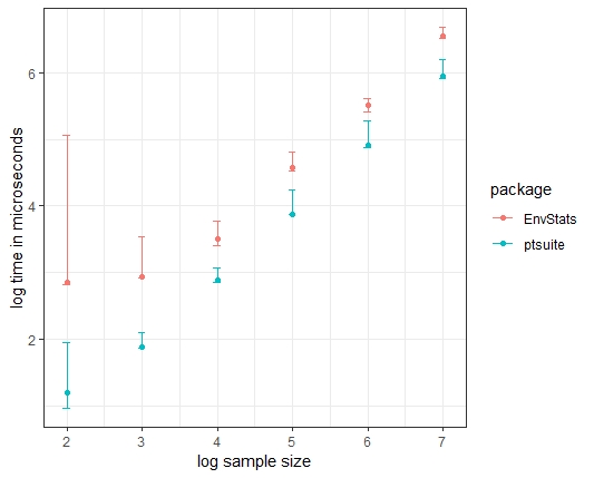
Table 6: Function timing results using \pkgmicrobenchmark for LS Estimate with sample 4.

Sample Size	Package	Mean ( $\mu$ s)	Maximum ( $\mu$ s)	Median ( $\mu$ s)	Minimum ( $\mu$ s)
$10^{2}$	ptsuite	2.02E+01	8.80E+01	1.55E+01	9.20E+00
$10^{2}$	EnvStats	2.10E+03	1.17E+05	7.23E+02	6.65E+02
$10^{3}$	ptsuite	7.83E+01	1.28E+02	7.73E+01	7.28E+01
$10^{3}$	EnvStats	9.06E+02	3.47E+03	8.65E+02	8.19E+02
$10^{4}$	ptsuite	7.81E+02	1.20E+03	7.73E+02	7.26E+02
$10^{4}$	EnvStats	3.19E+03	5.84E+03	3.20E+03	2.52E+03
$10^{5}$	ptsuite	7.84E+03	1.73E+04	7.56E+03	7.34E+03
$10^{5}$	EnvStats	4.12E+04	6.60E+04	3.77E+04	3.42E+04
$10^{6}$	ptsuite	9.45E+04	1.91E+05	8.06E+04	7.66E+04
$10^{6}$	EnvStats	3.28E+05	4.15E+05	3.23E+05	2.63E+05
$10^{7}$	ptsuite	9.17E+05	1.61E+06	8.79E+05	8.09E+05
$10^{7}$	EnvStats	3.66E+06	4.87E+06	3.62E+06	3.34E+06

Table 7: Function timing results using \pkgmicrobenchmark for generating Pareto data with sample 5.

Sample Size	Package	Mean ( $\mu$ s)	Maximum ( $\mu$ s)	Median ( $\mu$ s)	Minimum ( $\mu$ s)
$10^{2}$	ptsuite	2.02E+01	2.71E+01	2.00E+01	1.79E+01
	EnvStats	4.89E+02	3.23E+03	4.48E+02	4.07E+02
	evir	1.97E+01	3.87E+01	1.93E+01	1.86E+01
$10^{3}$	ptsuite	1.60E+02	1.91E+02	1.59E+02	1.56E+02
	EnvStats	3.63E+03	5.44E+03	3.51E+03	3.24E+03
	evir	1.62E+02	1.96E+02	1.61E+02	1.59E+02
$10^{4}$	ptsuite	1.55E+03	1.60E+03	1.55E+03	1.54E+03
	EnvStats	3.58E+04	7.29E+04	3.52E+04	3.23E+04
	evir	1.57E+03	1.62E+03	1.57E+03	1.56E+03
$10^{5}$	ptsuite	1.61E+04	2.33E+04	1.56E+04	1.54E+04
	EnvStats	3.62E+05	4.05E+05	3.58E+05	3.31E+05
	evir	1.57E+04	2.42E+04	1.56E+04	1.56E+04
$10^{6}$	ptsuite	1.59E+05	2.11E+05	1.56E+05	1.55E+05
	EnvStats	3.69E+06	4.02E+06	3.67E+06	3.59E+06
	evir	1.61E+05	1.79E+05	1.60E+05	1.58E+05
$10^{7}$	ptsuite	1.57E+06	1.68E+06	1.56E+06	1.55E+06
	EnvStats	3.67E+07	4.00E+07	3.64E+07	3.59E+07
	evir	1.60E+06	1.67E+06	1.60E+06	1.59E+06

3.1 Comparison of Estimation Methods within ptsuite package

In this section, we compare and present the speed of the (estimation method) functions available in the package \pkgptsuite using the package \pkgmicrobenchmark (Mersmann 2018). We do not include Hill’s Estimator as it restricts the domain to a subset of the sample. The results of this comparison can be seen in Table 8.

We note here that the most computationally intensive functions are the LS and the WLS methods with the WLS method consuming a very large time for progressively larger datasets. It is seen that the PM and the MPM are consistently the fastest methods regardless of the sample size (but we remind the reader that the results of the percentile methods are also the least accurate for small sample sizes).

Table 8: Function timing results using \pkgmicrobenchmark for various sample sizes.

Method	Sample Size	Minimum ( $\mu$ s)	Median ( $\mu$ s)	Maximum ( $\mu$ s)
MLE	$10^{3}$	2.36E+01	2.45E+01	5.77E+01
	$10^{4}$	2.20E+02	2.23E+02	3.55E+02
	$10^{5}$	2.17E+03	2.23E+03	2.63E+03
	$10^{6}$	2.19E+04	2.23E+04	2.33E+04
	$10^{7}$	2.22E+05	2.30E+05	2.50E+05
LS	$10^{3}$	5.46E+01	5.63E+01	8.53E+01
	$10^{4}$	5.44E+02	5.92E+02	6.81E+02
	$10^{5}$	5.56E+03	5.82E+03	1.83E+04
	$10^{6}$	5.88E+04	5.96E+04	7.32E+04
	$10^{7}$	6.27E+05	6.79E+05	7.53E+05
WLS	$10^{3}$	5.09E+01	5.26E+01	9.79E+01
	$10^{4}$	5.17E+02	5.39E+02	7.50E+02
	$10^{5}$	5.20E+03	5.38E+03	5.78E+03
	$10^{6}$	7.70E+04	7.82E+04	1.04E+05
	$10^{7}$	3.12E+07	3.53E+07	3.70E+07
PM	$10^{3}$	6.83E+00	7.40E+00	7.14E+01
	$10^{4}$	7.08E+01	7.20E+01	1.04E+02
	$10^{5}$	8.01E+02	8.17E+02	1.36E+03
	$10^{6}$	9.37E+03	9.66E+03	1.18E+04
	$10^{7}$	1.30E+05	1.36E+05	7.45E+05
MPM	$10^{3}$	7.11E+00	7.54E+00	8.16E+01
	$10^{4}$	7.05E+01	7.23E+01	1.52E+02
	$10^{5}$	8.02E+02	8.15E+02	1.11E+03
	$10^{6}$	9.35E+03	9.66E+03	2.44E+04
	$10^{7}$	1.30E+05	1.36E+05	1.88E+05
GMPM	$10^{3}$	2.90E+01	3.02E+01	1.12E+02
	$10^{4}$	2.93E+02	2.95E+02	6.61E+02
	$10^{5}$	3.03E+03	3.07E+03	4.19E+03
	$10^{6}$	3.19E+04	3.24E+04	8.90E+04
	$10^{7}$	3.55E+05	3.72E+05	4.34E+05
MoM	$10^{3}$	2.56E+01	2.70E+01	1.83E+02
	$10^{4}$	2.39E+02	2.44E+02	3.44E+02
	$10^{5}$	2.36E+03	2.42E+03	2.81E+03
	$10^{6}$	2.40E+04	2.43E+04	6.68E+04
	$10^{7}$	2.42E+05	2.52E+05	2.79E+05

4 Results for Accuracy

We begin by noting that we test the HE method separately as we have to supply an extra parameter, namely the tuning parameter $k$ . To test each of the other six methods methods we do the following:

1.

Simulate Pareto data for 4 different values of $\alpha$ : 0.5, 1.5, 2.2, 5. Pareto data is generated via

$x_{i}=\frac{x_{\mathrm{min}}}{u_{i}^{1/\alpha}}$

where $u_{i}$ is a standard uniform random number. We work with $x_{\mathrm{min}}=2$ for all the tests.
2.

For each $\alpha$ value we generate 3 different sample sizes: $10^{3},10^{5},10^{6}$ to test the effect of sample size on the accuracy.
3.

For each sample size we generate four different samples (by changing the random number generator seed).

In total we run $288=6\times 4\times 3\times 4$ tests. To economize on space we present a sample of the results (Table 9) with the complete set of results given in Appendix A. The $\hat{\alpha}$ error given is calculated as follows:

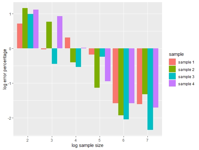
\mathrm{Error\,\%}=\frac{|\alpha-\hat{\alpha}|}{\alpha}\times 100\%

We also remark here that for the LS and PM methods, there is a peculiarity in that the accuracy dips slightly for particular increases in sample size. The reader is referred to Figure 8 to observe the counter-intuitive behavior⁷⁷ 7 Note that the error percentages are in log scale - hence larger negative bars indicate smaller error.. For example when considering sample 1, the LS $\alpha$ -estimate with $10^{3}$ samples has error $0.95\%$ and an error of $2.08\%$ with $10^{4}$ samples. When we increase the sample size to $10^{5}$ , the error drops as expected. Similarly for sample 1, the PM $\alpha$ -estimate with $10^{4}$ samples has error $0.07\%$ and an error of $0.85\%$ with $10^{5}$ samples. As with the LS method, when we increase the sample size to $10^{6}$ , the error drops as expected. We are not certain as to the reason for the drop in accuracy for a certain values of larger samples - we consider other samples (by changing the seed) and these results are presented in Appendix C and Appendix D respectively. The other samples also have this counter-intuitive behavior but at different sample sizes.

Method	Sample Size	$\hat{\alpha}$	$\hat{\alpha}$ error
MLE	$10^{2}$	2.52705	14.87%
	$10^{3}$	2.22869	1.30%
	$10^{4}$	2.18519	0.67%
	$10^{5}$	2.19168	0.38%
	$10^{6}$	2.19971	0.01%
	$10^{7}$	2.19954	0.02%
LS	$10^{2}$	2.31566	5.26%
	$10^{3}$	2.22096	0.95%
	$10^{4}$	2.15422	2.08%
	$10^{5}$	2.18542	0.66%
	$10^{6}$	2.20057	0.03%
	$10^{7}$	2.19946	0.02%
MoM	$10^{2}$	2.62537	19.34%
	$10^{3}$	2.28164	3.71%
	$10^{4}$	2.18505	0.68%
	$10^{5}$	2.19049	0.43%
	$10^{6}$	2.19942	0.03%
	$10^{7}$	2.20004	0.00%
PM	$10^{2}$	2.7422	24.65%
	$10^{3}$	2.27278	3.31%
	$10^{4}$	2.20158	0.07%
	$10^{5}$	2.18126	0.85%
	$10^{6}$	2.19776	0.10%
	$10^{7}$	2.20044	0.02%

Table 9: Sample results for

\alpha

= 2.2 (using sample 1 from each run). The sample sizes are

10^{3},10^{4},10^{5},10^{6}

and

10^{7}

4.1 Accuracy of Hill’s Estimator - Results

The HE method differs from the other methods in this paper as one needs to specify a cut-off point from which to consider the “tail” portion of the distribution. This is denoted by the \codek value which is the $k^{th}$ largest observation of the data set. In other words, it can be thought of as the number of observations of the tail to be considered in estimating the shape parameter (tail index). We may also specify a value as a starting point of the tail estimation area instead of a ranked order.

4.2 Hill’s Estimator for Strictly Pareto data

In this section we look at the impact of \codek when HE is used on strictly Pareto data. We consider the same random Pareto samples (with $\alpha=0.5,1.5,2.2$ and $5.0$ ) used for the previous estimators but only consider $10^{3},10^{5}$ and $10^{6}$ sample sizes along with \codek set at the $25^{th}$ , $50^{th}$ and $75^{th}$ percentiles for each sample size. (Refer Appendix B for the full set of results.)

We also generate four samples from the Pareto distribution with $\alpha=1.5$ and $\hat{x}_{\mathrm{min}}=5$ . Figure 9(b) shows how the HE varies with \codek. Since the data supplied is strictly Pareto, increasing \codek (from 1 to \coden = 100,000) increases the accuracy of the estimate and we can see the estimate stabilizing around $\hat{\alpha}=1.5$ .

4.3 Hill’s Estimator for Non-Pareto data

To further test the accuracy of the HE method and understand the relationship of the value of \codek in estimating $\alpha$ , we vary \codek in the presence of non-Pareto power law data. We consider data sampled from a i) t-distribution and ii) stable distribution respectively, and estimate the tail-index.

For this purpose we first generate four samples from the t-distribution with degrees of freedom (d.f.) equal to 3. The tail index $\alpha$ is estimated by varying \codek from 1 to \coden (where \coden = 100,000). It can be seen from Figure 10(b) that using a smaller value of \codek results in a more accurate estimation of the tail index - we feel this is because a smaller value of \codek avoids including observations from the “body” of the distribution. We should note however the earlier point about the bias of the estimator for small \codek.

Next we simulate four samples from a symmetric stable distribution⁸⁸ 8 A symmetric stable distribution was generated using $\frac{\sin(\alpha V)}{(\cos(V))^{1/\alpha}}(\frac{\cos((1-\alpha)V)}{W})^{(1-\alpha)/\alpha}$ where $V\sim Unif[-\pi/2,\pi/2]$ and $W\sim Exp(1)$ (Glasserman 2004, p.149). with stability parameter⁹⁹ 9 A symmetric stable distribution with stability parameter $\alpha$ has the following property $\lim_{x\rightarrow\pm\infty}p(x)\sim|x|^{1+\alpha}$ . (tail index) $\alpha$ =1.5 and vary \codek to estimate $\alpha$ . The results of this simulation are similar to that of t-distribution in that a smaller value of \codek leads to a closer estimate of the true $\alpha$ . The results are as follows:

5 Using the ptsuite Package

The \pkgptsuite is built with ease of use in mind. Here we go over the use of each of the functions provided in the package. The \pkgptsuite is available on Centralized R Archive Network (CRAN): https://cran.r-project.org/web/packages/ptsuite/index.html.

5.1 The \codegenerate_pareto function

This function is able to generate random Pareto distributed data with the specified \codeshape and \codescale parameters. The function has been written to be similar in type to the popular \coderunif and \coderexp type of functions for generating data from a particular distribution.

The full call of the function is: {Code} generate_pareto(sampleSize, shape, scale)

For example to generate a sample of size $100,000$ with $\alpha$ (shape parameter) = 1.2 and $x_{min}$ (scale parameter) = 3 and store it in the variable \codedata, the following code could be used: {CodeChunk} {CodeInput} R> set.seed(1234) R> d <- generate_pareto(100000, 1.2, 3) R> head(d)

This produces the following output: {CodeOutput} [1] 18.364397 4.454392 4.533604 4.447960 3.398763 4.349730

5.2 The \codepareto_qq_test function

The \codepareto_qq_test function can be used as a first step to identify whether the data is Pareto distributed before estimating the tail index. If most of the data points appear to be distributed along a line, it is possible that the data may be Pareto. Conversely, if most of the data are distributed non-linearly, then the data is most probably not Pareto distributed.

This function¹⁰¹⁰ 10 For added interactivity this package makes use of the \pkgplotly package (Sievert 2018) to generate the Q-Q plots if it is available in the user’s \proglangR library. If unavailable, it defaults to the \proglangR base plot. plots the quantiles of the standard exponential distribution on the x-axis and the log values of the provided data on the y-axis. If Pareto data was supplied, a log transformation of this data would result in an exponential distribution with mean $\alpha^{-1}$ . These data points would then show up on the QQ-plot as line with slope $\alpha^{-1}$ .

Note: This is a heuristic test where one can look for data being distributed along a straight line indicating a possible Pareto distribution.

The full call of the function is: {Code} pareto_qq_test(dat)

Demonstration of this function is carried out using a Pareto distributed sample of size $100,000$ with $\alpha$ (shape parameter) = 1.2 and $x_{min}$ (scale parameter) = 3, and using an exponentially distributed sample of size $100,000$ with $\lambda$ (reciprocal of mean) = 5 as an example of non-Pareto data.

Q-Q Plot constructed for Pareto distributed data: {CodeChunk} {CodeInput} R> set.seed(1234) R> d <- generate_pareto(100000, 1.2, 3) R> pareto_qq_test(d)

Q-Q Plot constructed for exponentially distributed data: {CodeChunk} {CodeInput} R> set.seed(1234) R> exp_data <- rexp(100000, 5) R> pareto_qq_test(exp_data)

5.3 The \codepareto_test function

The \codepareto_test function can be used to identify whether the data is Pareto distributed (Gulati and Shapiro 2008). The test generates a p-value corresponding to the actual distribution of the data and is tested for significance. In the case of Pareto data, the p-value should be greater than the pre-determined significance level (generally taken as $0.05$ ). In addition to using the function on Pareto data, we tested the function on selected non-Pareto (generated) data sets to ensure the test would reject those as Pareto. The tests were conducted on generated data sets of various sizes. The results¹¹¹¹ 11 In the table, half-normal distribution is taken to be the positive tail of the standard normal distribution excluding zeros. obtained are shown in Table 10.

Distribution	Sample Size	p-value
Pareto (shape = 1.2, scale = 3)	$10^{2}$	0.5056804
	$10^{3}$	0.1595162
	$10^{5}$	0.849023
Exponential (rate = 5)	$10^{2}$	$4.76\times 10^{-43}$
	$10^{3}$	0
	$10^{5}$	0
Binomial (n = 20, p = 0.6)	$10^{2}$	$1.06\times 10^{-44}$
	$10^{3}$	0
	$10^{5}$	0
Normal (mean = 5, std = 3); positive tail	$10^{2}$	$1.26\times 10^{-104}$
	$10^{3}$	0
	$10^{5}$	0

Table 10: Results of \codepareto_test function for various sample sizes.

The full call of the function is: {Code} pareto_test(dat)

{CodeChunk}{CodeInput}

R> set.seed(1234) R> d <- generate_pareto(100000, 1.2, 3) R> pareto_test(d)

{CodeOutput}

$`p-value`[1]0.8604162\par\CodeInput R>set.seed(1234)R>exp_{d}ata<-rexp(100000,5)R>pareto_{t}est(exp_{d}ata)\CodeOutput$`p-value`[1]0\par\par$

5.4 The \codealpha_mle function

This function can be used to estimate the shape parameter ( $\alpha$ ) using the Maximum Likelihood Estimator method - please refer equation (3). It can be used to obtain biased and unbiased estimates of the shape and scale parameters as well as the confidence interval for the shape parameter for the biased estimates.

The full call of the function is: {Code} alpha_mle(dat, biased = TRUE, significance = NULL)

To demonstrate the various possibilities of this function we first generate Pareto data with $\alpha=1.2$ and $x_{min}=3$ and assign it to the variable \codedata. \codealpha_mle is then used to obtain:

1.

Biased Estimates for $\alpha$ and $x_{min}$
2.

Unbiased Estimates for $\alpha$ and $x_{min}$
3.

Biased Estimates for $\alpha$ and $x_{min}$ and the $95\%$ confidence interval for $\alpha$

R implementation of the above mentioned demonstration is given below.

Generating data from a Pareto Distribution: {CodeChunk} {CodeInput} R> set.seed(1234) R> d <- generate_pareto(100000, 1.2, 3) Obtaining the biased maximum likelihood estimates for $\alpha$ and $x_{min}$ : {CodeInput} R> alpha_mle(d) {CodeOutput} $shape[1]1.201384\par$ scale [1] 3.000005

Obtaining the unbiased maximum likelihood estimates for $\alpha$ and $x_{min}$ : {CodeInput} R> alpha_mle(d, FALSE) {CodeOutput} $shape[1]1.201359\par$ scale [1] 2.99998

Obtaining the biased maximum likelihood estimator for $\alpha$ and $x_{min}$ and the corresponding $95\%$ confidence interval for $\alpha$ : {CodeInput} R> alpha_mle(d, TRUE, 0.05) {CodeOutput} $shape[1]1.201384\par$ lower_bound [1] 1.193937

$upper_{b}ound[1]1.20883\par$ scale [1] 3.000005

5.5 The \codealpha_hills function

The Hill’s Estimator - please refer equation (13) - is particularly useful in the fact that it allows the specification of \codek as either the number of observations to be included in the tail (where \codevalue = FALSE) or the minimum value to be considered in the tail of the distribution (where \codevalue = TRUE). When \codek=\coden, the Hill’s Estimator returns the same estimate as \codealpha_mle with a warning notifying the user.

The full call of the function is: {Code} alpha_hills(dat, k, value = FALSE)

We demonstrate the usage of the Hill’s Estimator by generating Pareto data with $\alpha$ =1.2 and $x_{min}$ =3, assigning it to the variable \codedata and then using \codealpha_hills

R implementation of the above mentioned demonstration is given below with the respective outputs: {CodeChunk} {CodeInput} R> set.seed(1234) R> d <- generate_pareto(100000, 1.2, 3) R> alpha_hills(d, 8000, FALSE) {CodeOutput} $shape[1]1.198717\par$ scale [1] 24.54499

{CodeInput}

R> alpha_hills(d, 5000, TRUE) {CodeOutput} $shape[1]1.125696\par$ scale [1] 5002.76

{CodeInput}

R> alpha_hills(d, 100000, FALSE) {CodeOutput} $shape[1]1.201384\par$ scale [1] 3.000005

Warning message: In alpha_hills(d, 1e+05, FALSE) : Setting k as the number of observations makes it equivalent to the MLE (alpha_mle function).

5.6 The \codealpha_ls function

This function can be used to estimate the shape parameter ( $\alpha$ ) using the Least Squares Estimator method - please refer equation (5).

The full call of the function is: {Code} alpha_ls(dat)

We demonstrate the usage of the Least Squares Estimator by generating Pareto data with $\alpha$ =1.2 and $x_{min}$ =3, assigning it to the variable \codedata and then using \codealpha_ls.

R implementation of the above mentioned demonstration is given below with the respective output: {CodeChunk} {CodeInput} R> set.seed(1234) R> d <- generate_pareto(100000, 1.2, 3) R> alpha_ls(d)

{CodeOutput}

$shape[1]1.20067\par$ scale [1] 3.000005

5.7 The \codealpha_percentile function

This function can be used to estimate the shape parameter ( $\alpha$ ) using the Percentile Estimator method - please refer equation (9).

The full call of the function is: {Code} alpha_percentile(dat)

We demonstrate the usage of the Percentile Estimator by generating Pareto data with $\alpha$ =1.2 and $x_{min}$ =3, assigning it to the variable \codedata and then using \codealpha_percentile.

{CodeOutput}

$shape[1]1.20048\par$ scale [1] 3.000005

5.8 The \codealpha_modified_percentile function

This function can be used to estimate the shape parameter ( $\alpha$ ) using the Modified Percentile Estimator method - please refer equation (10).

The full call of the function is: {Code} alpha_modified_percentile(dat)

We demonstrate the usage of the Modified Percentile Estimator by generating Pareto data with $\alpha$ =1.2 and $x_{min}$ =3, assigning it to the variable \codedata and then using
\codealpha_modified_percentile.

{CodeOutput}

$shape[1]1.196936\par$ scale [1] 3.000005

5.9 The \codealpha_geometric_percentile function

This function can be used to estimate the shape parameter ( $\alpha$ ) using the Geometric Percentile Estimator method - please refer equation (11).

The full call of the function is: {Code} alpha_geometric_percentile(dat)

We demonstrate the usage of the Geometric Percentile Estimator by generating Pareto data with $\alpha$ =1.2 and $x_{min}$ =3, assigning it to the variable \codedata and then using
\codealpha_geometric_percentile.

{CodeOutput}

$shape[1]1.195801\par$ scale [1] 3.000005

5.10 The \codealpha_wls function

This function can be used to estimate the shape parameter ( $\alpha$ ) using the Weighted Least Squares Estimator method - please refer to equations (7) and (8).

The full call of the function is: {Code} alpha_wls(dat)

We demonstrate the usage of the Weighted Least Squares Estimator by generating Pareto data with $\alpha$ =1.2 and $x_{min}$ =3, assigning it to the variable \codedata and then using \codealpha_wls.

5.11 The \codealpha_moment function

This function can be used to estimate the shape parameter ( $\alpha$ ) using the Moment Estimator method - please refer equation (12).

The full call of the function is: {Code} alpha_moment(dat)

We demonstrate the usage of the Moment Estimator by generating Pareto data with $\alpha$ =1.2 and $x_{min}$ =3, assigning it to the variable \codedata and then using \codealpha_moment.

5.12 The \codegenerate_all_estimates function

This function can be used to obtain estimates of the shape parameter ( $\alpha$ ) using all estimators except the HE.

The full call of the function is: {Code} generate_all_estimates(dat)

We demonstrate the usage of the function by generating Pareto data with $\alpha$ =1.2 and $x_{min}$ =3, assigning it to the variable \codedata and then using \codegenerate_all_estimates.

R implementation of the above mentioned demonstration is given below with the respective output: {CodeChunk} {CodeInput} R> set.seed(1234) R> d <- generate_pareto(100000, 1.2, 3) R> generate_all_estimates(d) {CodeOutput} Method.of.Estimation Shape.Parameter Scale.Parameter 1 Maximum Likelihood Estimate 1.201384 3.000005 2 Least Squares 1.200670 3.000005 3 Method of Moments 1.241772 3.000005 4 Percentiles Method 1.200480 3.000005 5 Modified Percentiles Method 1.196936 3.000005 6 Geometric Percentiles Method 1.195801 3.000005 7 Weighted Least Squares 1.201303 3.000005

6 Summary and Future Work

Our \proglangR package \pkgptsuite can be used in tail index estimation for Pareto distributed data. One may use the \codepareto-qq-test function as a first step to test (heuristically) if the data is Pareto. There are a number of methods which can be called on to estimate the tail index, and it is advisable to use more than one method as a comparison for the estimate.

Our main focus in developing this package was on run-times for parameter estimation for large data samples. The estimation methods on \pkgptsuite were faster than their counterpart methods in the packages \pkglaeken and \pkgEnvStats. The Pareto data generation function on \pkgptsuite was also faster than that of the package \pkgEnvStats. All functions on \pkgptsuite performed reasonably well in the speed tests, where we tested data sets with up to $10^{7}$ data points.

For future work we hope to add more tail estimation methods and functions found in the references to this package. In particular we hope to eventually incorporate the vast catalog of estimators in reference Fedotenkov 2018.

Computational details

The results in this paper were obtained using \proglangR 3.5.2. and Microsoft \proglangR 3.5.1 (Microsoft and Team 2017)¹²¹² 12 Microsoft \proglangR was used for the benchmark results of the speed and we note here that this version of \proglangR appeared to use slightly lower times in running the same tests. with the \pkgptsuite 1.0.0 package. \proglangR itself and all packages used are available from the Comprehensive \proglangR Archive Network (CRAN) at https://CRAN.R-project.org/. Microsoft \proglangR may be obtained from https://mran.microsoft.com/open.

RStudio V 1.1.423 (RStudio Team 2016) was used as the IDE for all tasks related to package development and generating results. The packages \pkgdevtools (Wickham et al. 2018b) and \pkgroxygen2 (Wickham et al. 2018a) were used to assist in package documentation and development. The \pkgRcpp package (Eddelbuettel and François 2011; Eddelbuettel 2013; Eddelbuettel and Balamuta 2017) was used in the compilation of \proglangC++ code used in all estimation functions of the package.

\pkg

microbenchmark 1.4-4, \pkgggplot2 3.0.0 (Wickham 2016) and \pkgplotly 4.8.0 were used in generating the results included in this paper.

Two computers were used in the building of this package and the generation of the results. The technical specifications of the two computers are as follows:

Specification

Laptop

Desktop

CPU

Intel(R) Core(TM) i5-8250U

@ 1.60GHz, 1800 Mhz,

4 Core(s), 8 Logical Processor(s)

Intel(R) Core(TM) i7-7700

@ 3.60GHz, 3601 Mhz,

4 Core(s), 8 Logical Processor(s)

RAM

8 GB

32 GB

Windows 10 Enterprise

LTSC 10.0.17763 Build 17763

Windows 10 Pro

10.0.17763 Build 17763

Acknowledgments

We wish to acknowledge Dr. J. Nair for helpful advice and in providing unpublished material for our research and Prof. S. Gulati for sharing knowledge on the Goodness of Fit tests. D. J. would also like to acknowledge Prof. S. Banneheka for a very useful discussion on the WLS method of estimation.

References

Bhatti et al. (2018) Bhatti SH, Hussain S, Ahmad T, Aslam M, Aftab M, Raza MA (2018). “Efficient estimation of Pareto model: Some modified percentile estimators.” PLoS ONE, 13(5), 1–15.
Brazauskas and Serfling (2000) Brazauskas V, Serfling R (2000). “Robust and Efficient Estimation Of The Tail Index Of A Single-Parameter Pareto Distribution.” North American Actuarial Journal, 4, 12–27.
Eddelbuettel (2013) Eddelbuettel D (2013). Seamless R and C++ Integration with Rcpp. Springer, New York. 10.1007/978-1-4614-6868-4. ISBN 978-1-4614-6867-7.
Eddelbuettel and Balamuta (2017) Eddelbuettel D, Balamuta JJ (2017). “Extending extitR with extitC++: A Brief Introduction to extitRcpp.” PeerJ Preprints, 5, e3188v1. ISSN 2167-9843. 10.7287/peerj.preprints.3188v1. URL https://doi.org/10.7287/peerj.preprints.3188v1.
Eddelbuettel and François (2011) Eddelbuettel D, François R (2011). “Rcpp: Seamless R and C++ Integration.” Journal of Statistical Software, 40(8), 1–18. 10.18637/jss.v040.i08. URL http://www.jstatsoft.org/v40/i08/.
Fedotenkov (2018) Fedotenkov I (2018). “A review of more than one hundred Pareto-tail index estimators.” MPRA Paper 90072, University Library of Munich, Germany. URL https://ideas.repec.org/p/pra/mprapa/90072.html.
Glasserman (2004) Glasserman P (2004). Monte Carlo Methods in Financial Engineering. Springer, New York, NY, USA.
Gulati and Shapiro (2008) Gulati S, Shapiro S (2008). “Goodness-of-Fit Tests for Pareto Distribution.” In F Vonta (ed.), Statistical Models and Methods for Biomedical and Technical Systems, chapter 19, pp. 259–274. Birkhäuser Basel. ISBN 978-0-8176-4619-6. 10.1007/978-0-8176-4619-6.
Hill (1975) Hill B (1975). “A Simple General Approach To Inference About The Tail Of A Distribution.” The Annals of Statistics, 3(5), 1163–1174.
Hubert et al. (2013) Hubert M, Dierckx G, Vanpaemal D (2013). “Detecting Influential Data Point For The Hill Estimator In Pareto-Type Distriubtions.” Computational Statistics & Data Analysis, 65, 13–28.
Mersmann (2018) Mersmann O (2018). microbenchmark: Accurate Timing Functions. R package version 1.4-4, URL https://CRAN.R-project.org/package=microbenchmark.
Microsoft and Team (2017) Microsoft, Team RC (2017). Microsoft R Open. Microsoft, Redmond, Washington. URL https://mran.microsoft.com/.
Munasinghe et al. (2020) Munasinghe RM, Kossinna P, Wijeratne D, Jayasinghe D (2020). “In Preparation.” Fat Tails and Power Laws in Business Data.
Nair et al. (2019) Nair J, Wierman A, Zwart B (2019). “The Fundamentals Of Heavy Tails: Properties, Emergence, And Identification.” Http://users.cms.caltech.edu/ adamw/heavytails.html.
Newman (2005) Newman MEJ (2005). “Power Laws, Pareto Distributions And Zipf’s Law.” Contemporary Physics, 46, 323–351.
Nolan (2017) Nolan JP (2017). “Stable Distributions: Models For Heavy Tailed Data.” Http://fs2.american.edu/jpnolan/www/stable/chap1.pdf.
Pokorna (2016) Pokorna M (2016). Estimation and Application of the Tail Index. Bachelor’s thesis, Charles University in Prague, Faculty of Social Sciences, Institute of Economic Studies.
R Core Team (2018) R Core Team (2018). R: A Language and Environment for Statistical Computing. R Foundation for Statistical Computing, Vienna, Austria. URL https://www.R-project.org/.
Rizzo (2009) Rizzo ML (2009). “New Goodness-of-Fit Tests for Pareto Distributions.” ASTIN Bulletin: The Journal Of The IAA, 39(2), 691–715.
RStudio Team (2016) RStudio Team (2016). RStudio: Integrated Development Environment for R. RStudio, Inc., Boston, MA. URL http://www.rstudio.com/.
Rytgaard (1990) Rytgaard M (1990). “Estimation In The Pareto Distribution.” ASTIN Bulletin: The Journal Of The IAA, 20(2), 201–216.
Sievert (2018) Sievert C (2018). plotly for R. URL https://plotly-book.cpsievert.me.
Sornette (2004) Sornette D (2004). Critical Phenomena In Natural Sciences, Chaos, Fractals, Selforganization And Disorder: Concepts And Tools. Springer Series in Synergetics.
Taleb (2019) Taleb NN (2019). The Statistical Consequences Of Fat Tails. Stem Academic Publishing.
Wickham (2016) Wickham H (2016). ggplot2: Elegant Graphics for Data Analysis. Springer-Verlag New York. ISBN 978-3-319-24277-4. URL http://ggplot2.org.
Wickham et al. (2018a) Wickham H, Danenberg P, Eugster M (2018a). roxygen2: In-Line Documentation for R. R package version 6.1.1, URL https://CRAN.R-project.org/package=roxygen2.
Wickham et al. (2018b) Wickham H, Hester J, Chang W (2018b). devtools: Tools to Make Developing R Packages Easier. R package version 2.0.1, URL https://CRAN.R-project.org/package=devtools.
Zaher et al. (2014) Zaher HM, El-Sheik AA, El-Magd NATA (2014). “Estimation of Pareto Parameters Using a Fuzzy Least-Squares Method and Other Known Techniques with a Comparison.” British Journal of Mathematics & Computer Science, 4(14), 2067–2088.
Zhang and Horvath (2005) Zhang B, Horvath S (2005). “A General Framework for Weighted Gene Co-Expression Network Analysis.” Statistical Applications in Genetics and Molecular Biology, 4(1), 1–43.

Appendix A Complete Tables of Estimates

Table 11: Sample results for

\alpha

= 5.0 (for all samples).

Method	Sample Size	Sample	$\hat{\alpha}$	$\hat{x}_{\mathrm{min}}$	$\hat{\alpha}$ error
MLE	$10^{3}$	1	5.0652128	2.000028	1.30%
		2	4.8768226	2.000292	2.46%
		3	5.1345472	2.000087	2.69%
		4	4.7497352	2.000301	5.01%
	$10^{5}$	1	4.9810971	2.000021	0.38%
		2	5.0083374	2.000011	0.17%
		3	4.9807569	2.000002	0.38%
		4	5.0034707	2.000001	0.07%
	$10^{6}$	1	4.9993293	2.000001	0.01%
		2	5.0041973	2.000000	0.08%
		3	4.9976888	2.000000	0.05%
		4	4.9974922	2.000000	0.05%
LS	$10^{3}$	1	5.0476293	2.000028	0.95%
		2	4.7059973	2.000292	5.88%
		3	5.0180434	2.000087	0.36%
		4	4.5705256	2.000301	8.59%
	$10^{5}$	1	4.9668545	2.000021	0.66%
		2	4.9963066	2.000011	0.07%
		3	4.9709030	2.000002	0.58%
		4	5.0056427	2.000001	0.11%
	$10^{6}$	1	5.0012983	2.000001	0.03%
		2	5.0005891	2.000000	0.01%
		3	4.9995475	2.000000	0.01%
		4	4.9986945	2.000000	0.03%
MoM	$10^{3}$	1	5.1021780	2.000028	2.04%
		2	4.8865050	2.000292	2.27%
		3	5.1537270	2.000087	3.07%
		4	4.7433810	2.000301	5.13%
	$10^{5}$	1	4.9795270	2.000021	0.41%
		2	5.0083190	2.000011	0.17%
		3	4.9799920	2.000002	0.40%
		4	5.0053840	2.000001	0.11%
	$10^{6}$	1	4.9999360	2.000001	0.00%
		2	5.0037260	2.000000	0.07%
		3	4.9984560	2.000000	0.03%
		4	4.9980840	2.000000	0.04%
PM	$10^{3}$	1	5.1654072	2.000028	3.31%
		2	4.5323446	2.000292	9.35%
		3	5.1056805	2.000087	2.11%
		4	4.8577159	2.000301	2.85%
	$10^{5}$	1	4.9574049	2.000021	0.85%
		2	4.9728086	2.000011	0.54%
		3	4.9921967	2.000002	0.16%
		4	4.9938595	2.000001	0.12%
	$10^{6}$	1	4.9949127	2.000001	0.10%
		2	4.9947259	2.000000	0.11%
		3	4.9959874	2.000000	0.08%
		4	4.9975729	2.000000	0.05%
MPM	$10^{3}$	1	5.5241262	2.000028	10.48%
		2	4.4701475	2.000292	10.60%
		3	4.9320572	2.000087	1.36%
		4	5.0637775	2.000301	1.28%
	$10^{5}$	1	4.9419910	2.000021	1.16%
		2	4.9524059	2.000011	0.95%
		3	4.9728058	2.000002	0.54%
		4	4.9907899	2.000001	0.18%
	$10^{6}$	1	4.9857602	2.000001	0.28%
		2	4.9911313	2.000000	0.18%
		3	4.9964677	2.000000	0.07%
		4	4.9969832	2.000000	0.06%
GMPM	$10^{3}$	1	5.2572589	2.000028	5.15%
		2	4.2810147	2.000292	14.38%
		3	5.1427862	2.000087	2.86%
		4	5.1208210	2.000301	2.42%
	$10^{5}$	1	4.9431381	2.000021	1.14%
		2	4.9554940	2.000011	0.89%
		3	5.0087703	2.000002	0.18%
		4	4.9784400	2.000001	0.43%
	$10^{6}$	1	4.9854361	2.000001	0.29%
		2	4.9928066	2.000000	0.14%
		3	4.9986738	2.000000	0.03%
		4	4.9955151	2.000000	0.09%
WLS	$10^{3}$	1	5.0430631	2.000028	0.86%
		2	4.8554967	2.000292	2.89%
		3	5.1120943	2.000087	2.24%
		4	4.7289651	2.000301	5.42%
	$10^{5}$	1	4.9807646	2.000021	0.38%
		2	5.0080031	2.000011	0.16%
		3	4.9804244	2.000002	0.39%
		4	5.0031367	2.000001	0.06%
	$10^{6}$	1	4.9992902	2.000001	0.01%
		2	5.0041581	2.000000	0.08%
		3	4.9976496	2.000000	0.05%
		4	4.9974531	2.000000	0.05%

Table 12: Sample results for

\alpha

= 2.2 (for all samples).

Method	Sample Size	Sample	$\hat{\alpha}$	$\hat{x}_{\mathrm{min}}$	$\hat{\alpha}$ error
MLE	$10^{3}$	1	2.2286936	2.000063	1.30%
		2	2.1458019	2.000664	2.46%
		3	2.2592007	2.000197	2.69%
		4	2.0898835	2.000683	5.01%
	$10^{5}$	1	2.1916827	2.000048	0.38%
		2	2.2036685	2.000025	0.17%
		3	2.1915330	2.000005	0.38%
		4	2.2015271	2.000002	0.07%
	$10^{6}$	1	2.1997049	2.000001	0.01%
		2	2.2018468	2.000000	0.08%
		3	2.1989831	2.000001	0.05%
		4	2.1988966	2.000000	0.05%
LS	$10^{3}$	1	2.2209569	2.000063	0.95%
		2	2.0706388	2.000664	5.88%
		3	2.2079391	2.000197	0.36%
		4	2.0110313	2.000683	8.59%
	$10^{5}$	1	2.1854160	2.000048	0.66%
		2	2.1983749	2.000025	0.07%
		3	2.1871973	2.000005	0.58%
		4	2.2024828	2.000002	0.11%
	$10^{6}$	1	2.2005712	2.000001	0.03%
		2	2.2002592	2.000000	0.01%
		3	2.1998009	2.000001	0.01%
		4	2.1994256	2.000000	0.03%
MoM	$10^{3}$	1	2.2816390	2.000063	3.71%
		2	2.1801250	2.000664	0.90%
		3	2.2992300	2.000197	4.51%
		4	2.0812090	2.000683	5.40%
	$10^{5}$	1	2.1904890	2.000048	0.43%
		2	2.2085240	2.000025	0.39%
		3	2.1897800	2.000005	0.46%
		4	2.2048300	2.000002	0.22%
	$10^{6}$	1	2.1994210	2.000001	0.03%
		2	2.2021380	2.000000	0.10%
		3	2.1998500	2.000001	0.01%
		4	2.2005870	2.000000	0.03%
PM	$10^{3}$	1	2.2727792	2.000063	3.31%
		2	1.9942276	2.000664	9.35%
		3	2.2464994	2.000197	2.11%
		4	2.1373945	2.000683	2.85%
	$10^{5}$	1	2.1812582	2.000048	0.85%
		2	2.1880358	2.000025	0.54%
		3	2.1965665	2.000005	0.16%
		4	2.1972982	2.000002	0.12%
	$10^{6}$	1	2.1977616	2.000001	0.10%
		2	2.1976794	2.000000	0.11%
		3	2.1982344	2.000001	0.08%
		4	2.1989321	2.000000	0.05%
MPM	$10^{3}$	1	2.4306180	2.000063	10.48%
		2	1.9668589	2.000664	10.60%
		3	2.1701057	2.000197	1.36%
		4	2.2280617	2.000683	1.28%
	$10^{5}$	1	2.1744760	2.000048	1.16%
		2	2.1790586	2.000025	0.95%
		3	2.1880345	2.000005	0.54%
		4	2.1959476	2.000002	0.18%
	$10^{6}$	1	2.1937345	2.000001	0.28%
		2	2.1960978	2.000000	0.18%
		3	2.1984458	2.000001	0.07%
		4	2.1986726	2.000000	0.06%
GMPM	$10^{3}$	1	2.3131938	2.000063	5.15%
		2	1.8836362	2.000664	14.38%
		3	2.2628257	2.000197	2.86%
		4	2.2531594	2.000683	2.42%
	$10^{5}$	1	2.1749808	2.000048	1.14%
		2	2.1804174	2.000025	0.89%
		3	2.2038589	2.000005	0.18%
		4	2.1905136	2.000002	0.43%
	$10^{6}$	1	2.1935919	2.000001	0.29%
		2	2.1968349	2.000000	0.14%
		3	2.1994165	2.000001	0.03%
		4	2.1980267	2.000000	0.09%
WLS	$10^{3}$	1	2.2189478	2.000063	0.86%
		2	2.1364185	2.000664	2.89%
		3	2.2493215	2.000197	2.24%
		4	2.0807446	2.000683	5.42%
	$10^{5}$	1	2.1915364	2.000048	0.38%
		2	2.2035214	2.000025	0.16%
		3	2.1913868	2.000005	0.39%
		4	2.2013802	2.000002	0.06%
	$10^{6}$	1	2.1996877	2.000001	0.01%
		2	2.2018296	2.000000	0.08%
		3	2.1989658	2.000001	0.05%
		4	2.1988794	2.000000	0.05%

Table 13: Sample results for

\alpha

= 1.5 (for all samples).

Method	Sample Size	Sample	$\hat{\alpha}$	$\hat{x}_{\mathrm{min}}$	$\hat{\alpha}$ error
MLE	$10^{3}$	1	1.5195638	2.000093	1.30%
		2	1.4630468	2.000974	2.46%
		3	1.5403641	2.000289	2.69%
		4	1.4249206	2.001002	5.01%
	$10^{5}$	1	1.4943291	2.000071	0.38%
		2	1.5025012	2.000037	0.17%
		3	1.4942271	2.000007	0.38%
		4	1.5010412	2.000002	0.07%
	$10^{6}$	1	1.4997988	2.000002	0.01%
		2	1.5012592	2.000001	0.08%
		3	1.4993066	2.000001	0.05%
		4	1.4992477	2.000000	0.05%
LS	$10^{3}$	1	1.5142888	2.000093	0.95%
		2	1.4117992	2.000974	5.88%
		3	1.5054130	2.000289	0.36%
		4	1.3711577	2.001002	8.59%
	$10^{5}$	1	1.4900564	2.000071	0.66%
		2	1.4988920	2.000037	0.07%
		3	1.4912709	2.000007	0.58%
		4	1.5016928	2.000002	0.11%
	$10^{6}$	1	1.5003895	2.000002	0.03%
		2	1.5001767	2.000001	0.01%
		3	1.4998643	2.000001	0.01%
		4	1.4996084	2.000000	0.03%
MoM	$10^{3}$	1	1.5974170	2.000093	6.49%
		2	1.5323020	2.000974	2.15%
		3	1.6119070	2.000289	7.46%
		4	1.4335130	2.001002	4.43%
	$10^{5}$	1	1.4960330	2.000071	0.26%
		2	1.5201780	2.000037	1.35%
		3	1.4872030	2.000007	0.85%
		4	1.5105550	2.000002	0.70%
	$10^{6}$	1	1.4956750	2.000002	0.29%
		2	1.5064640	2.000001	0.43%
		3	1.5007780	2.000001	0.05%
		4	1.5062520	2.000000	0.42%
PM	$10^{3}$	1	1.5496222	2.000093	3.31%
		2	1.3596983	2.000974	9.35%
		3	1.5317042	2.000289	2.11%
		4	1.4573142	2.001002	2.85%
	$10^{5}$	1	1.4872215	2.000071	0.85%
		2	1.4918426	2.000037	0.54%
		3	1.4976590	2.000007	0.16%
		4	1.4981578	2.000002	0.12%
	$10^{6}$	1	1.4984738	2.000002	0.10%
		2	1.4984178	2.000001	0.11%
		3	1.4987962	2.000001	0.08%
		4	1.4992719	2.000000	0.05%
MPM	$10^{3}$	1	1.6572410	2.000093	10.48%
		2	1.3410367	2.000974	10.60%
		3	1.4796178	2.000289	1.36%
		4	1.5191328	2.001002	1.28%
	$10^{5}$	1	1.4825973	2.000071	1.16%
		2	1.4857218	2.000037	0.95%
		3	1.4918417	2.000007	0.54%
		4	1.4972370	2.000002	0.18%
	$10^{6}$	1	1.4957281	2.000002	0.28%
		2	1.4973394	2.000001	0.18%
		3	1.4989403	2.000001	0.07%
		4	1.4990950	2.000000	0.06%
GMPM	$10^{3}$	1	1.5771776	2.000093	5.15%
		2	1.2842916	2.000974	14.38%
		3	1.5428356	2.000289	2.86%
		4	1.5362441	2.001002	2.42%
	$10^{5}$	1	1.4829414	2.000071	1.14%
		2	1.4866482	2.000037	0.89%
		3	1.5026311	2.000007	0.18%
		4	1.4935320	2.000002	0.43%
	$10^{6}$	1	1.4956308	2.000002	0.29%
		2	1.4978420	2.000001	0.14%
		3	1.4996021	2.000001	0.03%
		4	1.4986545	2.000000	0.09%
WLS	$10^{3}$	1	1.5129189	2.000093	0.86%
		2	1.4566490	2.000974	2.89%
		3	1.5336283	2.000289	2.24%
		4	1.4186895	2.001002	5.42%
	$10^{5}$	1	1.4942294	2.000071	0.38%
		2	1.5024009	2.000037	0.16%
		3	1.4941273	2.000007	0.39%
		4	1.5009410	2.000002	0.06%
	$10^{6}$	1	1.4997871	2.000002	0.01%
		2	1.5012474	2.000001	0.08%
		3	1.4992949	2.000001	0.05%
		4	1.4992359	2.000000	0.05%

Table 14: Sample results for

\alpha

= 0.5 (for all samples).

Method	Sample Size	Sample	$\hat{\alpha}$	$\hat{x}_{\mathrm{min}}$	$\hat{\alpha}$ error
MLE	$10^{3}$	1	0.5065213	2.000278	1.30%
		2	0.4876823	2.002923	2.46%
		3	0.5134547	2.000866	2.69%
		4	0.4749735	2.003009	5.01%
	$10^{5}$	1	0.4981097	2.000212	0.38%
		2	0.5008337	2.000112	0.17%
		3	0.4980757	2.000021	0.38%
		4	0.5003471	2.000007	0.07%
	$10^{6}$	1	0.4999329	2.000007	0.01%
		2	0.5004197	2.000002	0.08%
		3	0.4997689	2.000004	0.05%
		4	0.4997492	2.000000	0.05%
LS	$10^{3}$	1	0.5047629	2.000278	0.95%
		2	0.4705997	2.002923	5.88%
		3	0.5018043	2.000866	0.36%
		4	0.4570526	2.003009	8.59%
	$10^{5}$	1	0.4966855	2.000212	0.66%
		2	0.4996307	2.000112	0.07%
		3	0.4970903	2.000021	0.58%
		4	0.5005643	2.000007	0.11%
	$10^{6}$	1	0.5001298	2.000007	0.03%
		2	0.5000589	2.000002	0.01%
		3	0.4999548	2.000004	0.01%
		4	0.4998695	2.000000	0.03%
MoM	$10^{3}$	1	1.0007560	2.000278	100.15%
		2	1.0003550	2.002923	100.07%
		3	1.0014970	2.000866	100.30%
		4	1.0000360	2.003009	100.01%
	$10^{5}$	1	1.0000010	2.000212	100.00%
		2	1.0000100	2.000112	100.00%
		3	1.0000000	2.000021	100.00%
		4	1.0000030	2.000007	100.00%
	$10^{6}$	1	1.0000000	2.000007	100.00%
		2	1.0000000	2.000002	100.00%
		3	1.0000000	2.000004	100.00%
		4	1.0000010	2.000000	100.00%
PM	$10^{3}$	1	0.5165408	2.000278	3.31%
		2	0.4532280	2.002923	9.35%
		3	0.5105681	2.000866	2.11%
		4	0.4857708	2.003009	2.85%
	$10^{5}$	1	0.4957405	2.000212	0.85%
		2	0.4972809	2.000112	0.54%
		3	0.4992197	2.000021	0.16%
		4	0.4993859	2.000007	0.12%
	$10^{6}$	1	0.4994913	2.000007	0.10%
		2	0.4994726	2.000002	0.11%
		3	0.4995987	2.000004	0.08%
		4	0.4997573	2.000000	0.05%
MPM	$10^{3}$	1	0.5524166	2.000278	10.48%
		2	0.4470051	2.002923	10.60%
		3	0.4932065	2.000866	1.36%
		4	0.5063772	2.003009	1.28%
	$10^{5}$	1	0.4941991	2.000212	1.16%
		2	0.4952406	2.000112	0.95%
		3	0.4972806	2.000021	0.54%
		4	0.4990790	2.000007	0.18%
	$10^{6}$	1	0.4985760	2.000007	0.28%
		2	0.4991131	2.000002	0.18%
		3	0.4996468	2.000004	0.07%
		4	0.4996983	2.000000	0.06%
GMPM	$10^{3}$	1	0.5257258	2.000278	5.15%
		2	0.4280850	2.002923	14.38%
		3	0.5142783	2.000866	2.86%
		4	0.5120792	2.003009	2.42%
	$10^{5}$	1	0.4943138	2.000212	1.14%
		2	0.4955494	2.000112	0.89%
		3	0.5008770	2.000021	0.18%
		4	0.4978440	2.000007	0.43%
	$10^{6}$	1	0.4985436	2.000007	0.29%
		2	0.4992807	2.000002	0.14%
		3	0.4998674	2.000004	0.03%
		4	0.4995515	2.000000	0.09%
WLS	$10^{3}$	1	0.5043063	2.000278	0.86%
		2	0.4855497	2.002923	2.89%
		3	0.5112094	2.000866	2.24%
		4	0.4728965	2.003009	5.42%
	$10^{5}$	1	0.4980765	2.000212	0.38%
		2	0.5008003	2.000112	0.16%
		3	0.4980424	2.000021	0.39%
		4	0.5003137	2.000007	0.06%
	$10^{6}$	1	0.4999290	2.000007	0.01%
		2	0.5004158	2.000002	0.08%
		3	0.4997650	2.000004	0.05%

Appendix B Hill’s Estimates

Table 15: Sample results for

\alpha

= 5.0 (Hill’s Estimate).

Sample Size	\codek	Sample	$\hat{\alpha}$	$\hat{x}_{\mathrm{min}}$	$\hat{\alpha}$ error
$10^{3}$	250	1	5.1384879	2.622409	2.77%
		2	5.0187719	2.688776	0.38%
		3	5.1645221	2.619874	3.29%
		4	4.7188721	2.662987	5.62%
	500	1	5.358747	2.314142	7.17%
		2	4.7658326	2.301751	4.68%
		3	4.9729643	2.276799	0.54%
		4	4.84922	2.32247	3.02%
	750	1	5.1040343	2.120318	2.08%
		2	4.7126907	2.108961	5.75%
		3	5.0974016	2.112979	1.95%
		4	4.7370529	2.124039	5.26%
$10^{5}$	25,000	1	4.9723687	2.643396	0.55%
		2	5.0014969	2.639987	0.03%
		3	4.9550096	2.640709	0.90%
		4	5.0164426	2.639534	0.33%
	50,000	1	4.9599243	2.297478	0.80%
		2	4.9784265	2.295197	0.43%
		3	4.9626286	2.297129	0.75%
		4	5.0032577	2.297264	0.07%
	75,000	1	4.968077	2.117967	0.64%
		2	4.9870807	2.116682	0.26%
		3	4.9819341	2.119073	0.36%
		4	5.0027546	2.118298	0.06%
$10^{6}$	250,000	1	5.0046153	2.639683	0.09%
		2	5.0012057	2.638868	0.02%
		3	4.9950568	2.639315	0.10%
		4	4.9990826	2.639467	0.02%
	500,000	1	4.9958074	2.297068	0.08%
		2	4.9965736	2.296702	0.07%
		3	4.9951842	2.297432	0.10%
		4	4.9973861	2.297595	0.05%
	750,000	1	5.0002598	2.11851	0.01%
		2	4.9976201	2.117838	0.05%
		3	4.9951151	2.118314	0.10%
		4	4.9987034	2.118581	0.03%

Table 16: Sample results for

\alpha

= 2.2 (Hill’s Estimate).

Sample Size	\codek	Sample	$\hat{\alpha}$	$\hat{x}_{\mathrm{min}}$	$\hat{\alpha}$ error
$10^{3}$	250	1	2.2609347	3.702224	2.77%
		2	2.2082596	3.918605	0.38%
		3	2.2723897	3.694097	3.29%
		4	2.0763037	3.833704	5.62%
	500	1	2.3578487	2.786314	7.17%
		2	2.0969663	2.752523	4.68%
		3	2.1881043	2.685175	0.54%
		4	2.1336568	2.809155	3.02%
	750	1	2.2457751	2.283975	2.08%
		2	2.0735839	2.256266	5.75%
		3	2.2428567	2.266049	1.95%
		4	2.0843033	2.293095	5.26%
$10^{5}$	25,000	1	2.1878422	3.769907	0.55%
		2	2.2006586	3.758865	0.03%
		3	2.1802042	3.761201	0.90%
		4	2.2072347	3.7574	0.33%
	50,000	1	2.1823667	2.740923	0.80%
		2	2.1905077	2.734741	0.43%
		3	2.1835566	2.739976	0.75%
		4	2.2014334	2.740342	0.07%
	75,000	1	2.1859539	2.278224	0.64%
		2	2.1943155	2.275084	0.26%
		3	2.192051	2.280928	0.36%
		4	2.201212	2.279033	0.06%
$10^{6}$	250,000	1	2.2020307	3.757883	0.09%
		2	2.2005305	3.755245	0.02%
		3	2.197825	3.756693	0.10%
		4	2.1995964	3.757182	0.02%
	500,000	1	2.1981553	2.739811	0.08%
		2	2.1984924	2.738818	0.07%
		3	2.197881	2.740798	0.10%
		4	2.1988499	2.741238	0.05%
	750,000	1	2.2001143	2.279551	0.01%
		2	2.1989528	2.277909	0.05%
		3	2.1978506	2.279071	0.10%
		4	2.1994295	2.279726	0.03%

Table 17: Sample results for

\alpha

= 1.5 (Hill’s Estimate).

Sample Size	\codek	Sample	$\hat{\alpha}$	$\hat{x}_{\mathrm{min}}$	$\hat{\alpha}$ error
$10^{3}$	250	1	1.5415464	4.934745	2.77%
		2	1.5056316	5.363466	0.38%
		3	1.5493566	4.918864	3.29%
		4	1.4156616	5.193897	5.62%
	500	1	1.6076241	3.252596	7.17%
		2	1.4297498	3.194905	4.68%
		3	1.4918893	3.08091	0.54%
		4	1.454766	3.291777	3.02%
	750	1	1.5312103	2.429964	2.08%
		2	1.4138072	2.38685	5.75%
		3	1.5292205	2.402043	1.95%
		4	1.4211159	2.444209	5.26%
$10^{5}$	25,000	1	1.4917106	5.067623	0.55%
		2	1.5004491	5.045869	0.03%
		3	1.4865029	5.050468	0.90%
		4	1.5049328	5.042983	0.33%
	50,000	1	1.4879773	3.175178	0.80%
		2	1.493528	3.16468	0.43%
		3	1.4887886	3.173568	0.75%
		4	1.5009773	3.174191	0.07%
	75,000	1	1.4904231	2.420997	0.64%
		2	1.4961242	2.416103	0.26%
		3	1.4945802	2.425212	0.36%
		4	1.5008264	2.422256	0.06%
$10^{6}$	250,000	1	1.5013846	5.043935	0.09%
		2	1.5003617	5.038743	0.02%
		3	1.4985171	5.041592	0.10%
		4	1.4997248	5.042554	0.02%
	500,000	1	1.4987422	3.173289	0.08%
		2	1.4989721	3.171602	0.07%
		3	1.4985553	3.174965	0.10%
		4	1.4992158	3.175713	0.05%
	750,000	1	1.5000779	2.423064	0.01%
		2	1.499286	2.420505	0.05%
		3	1.4985345	2.422317	0.10%
		4	1.499611	2.423337	0.03%

Table 18: Sample results for

\alpha

= 0.5 (Hill’s Estimate).

Sample Size	\codek	Sample	$\hat{\alpha}$	$\hat{x}_{\mathrm{min}}$	$\hat{\alpha}$ error
$10^{3}$	250	1	0.5138488	30.042363	2.77%
		2	0.5018772	38.572395	0.38%
		3	0.5164522	29.753256	3.29%
		4	0.4718872	35.028376	5.62%
	500	1	0.5358747	8.602613	7.17%
		2	0.4765833	8.152935	4.68%
		3	0.4972964	7.311007	0.54%
		4	0.484922	8.917257	3.02%
	750	1	0.5104034	3.587069	2.08%
		2	0.4712691	3.399504	5.75%
		3	0.5097402	3.464835	1.95%
		4	0.4737053	3.65052	5.26%
$10^{5}$	25,000	1	0.4972369	32.535157	0.55%
		2	0.5001497	32.11795	0.03%
		3	0.495501	32.20586	0.90%
		4	0.5016443	32.062887	0.33%
	50,000	1	0.4959924	8.002846	0.80%
		2	0.4978427	7.923726	0.43%
		3	0.4962629	7.990674	0.75%
		4	0.5003258	7.995384	0.07%
	75,000	1	0.4968077	3.547502	0.64%
		2	0.4987081	3.526034	0.26%
		3	0.4981934	3.566063	0.36%
		4	0.5002755	3.553042	0.06%
$10^{6}$	250,000	1	0.5004615	32.081033	0.09%
		2	0.5001206	31.982071	0.02%
		3	0.4995057	32.036353	0.10%
		4	0.4999083	32.054697	0.02%
	500,000	1	0.4995807	7.988564	0.08%
		2	0.4996574	7.975831	0.07%
		3	0.4995184	8.001228	0.10%
		4	0.4997386	8.006891	0.05%
	750,000	1	0.500026	3.556597	0.01%
		2	0.499762	3.545339	0.05%
		3	0.4995115	3.553309	0.10%
		4	0.4998703	3.557801	0.03%

Appendix C LS Estimates

Table 19: Sample results for

\alpha

= 2.2 (LS Estimate).

Sample Size	Sample	$\hat{\alpha}$	$\hat{\alpha}$ error
$10^{2}$	1	2.31566	5.26%
	2	1.88102	14.50%
	3	1.98422	9.81%
	4	1.91018	13.17%
$10^{3}$	1	2.22096	0.95%
	2	2.07064	5.88%
	3	2.20794	0.36%
	4	2.01103	8.59%
$10^{4}$	1	2.15422	2.08%
	2	2.20883	0.40%
	3	2.20648	0.29%
	4	2.1769	1.05%
$10^{5}$	1	2.18542	0.66%
	2	2.19838	0.07%
	3	2.1872	0.58%
	4	2.20248	0.11%
$10^{6}$	1	2.20057	0.03%
	2	2.20026	0.01%
	3	2.1998	0.01%
	4	2.19943	0.03%
$10^{7}$	1	2.19946	0.02%
	2	2.19896	0.05%
	3	2.2001	0.00%
	4	2.20043	0.02%

Appendix D PM Estimates

Table 20: Sample results for

\alpha

= 2.2 (PM Estimate).

Sample Size	Sample	$\hat{\alpha}$	$\hat{\alpha}$ error
$10^{2}$	1	2.7422	24.65%
	2	1.90896	13.23%
	3	1.99232	9.44%
	4	2.23726	1.69%
$10^{3}$	1	2.27278	3.31%
	2	1.99423	9.35%
	3	2.2465	2.11%
	4	2.1374	2.85%
$10^{4}$	1	2.20158	0.07%
	2	2.18846	0.52%
	3	2.15231	2.17%
	4	2.19973	0.01%
$10^{5}$	1	2.18126	0.85%
	2	2.18804	0.54%
	3	2.19657	0.16%
	4	2.1973	0.12%
$10^{6}$	1	2.19776	0.10%
	2	2.19768	0.11%
	3	2.19823	0.08%
	4	2.19893	0.05%
$10^{7}$	1	2.20044	0.02%
	2	2.20077	0.03%
	3	2.19956	0.02%
	4	2.20107	0.05%

Appendix E A note on the Generalized Pareto Distribution and evir package

In this section we discuss briefly the \proglangR-package \pkgevir. The other packages and their respective functions considered in this paper are straight forward in that they work directly with Pareto distributions for data generation/tail index estimation. The \proglangR-package \pkgevir, on the other hand, works with the Generalized Pareto Distribution (GPD). The GPD has the following form for its probability density function:

g(x)=\frac{1}{\sigma}\left[1+\frac{\xi(x-\mu)}{\sigma}\right]^{-(1+1/\xi)}

(14)

The pdf (14) is defined for $x\geq\mu$ when $\xi>0$ and is then equivalent to the Pareto distribution when making the following identifications:

	$\displaystyle x_{\mathrm{min}}$	$\displaystyle=$	$\displaystyle\frac{\sigma}{\xi}=\mu$		(15)
	$\displaystyle\alpha$	$\displaystyle=$	$\displaystyle\frac{1}{\xi}$		(16)

To compare our package \pkgptsuite with \pkgevir we work with the transformations above. In particular to generate Pareto data, we call the function \codergpd in \pkgevir and input $\xi,\sigma,\mu$ in terms of the corresponding $x_{\mathrm{min}}$ and $\alpha$ . For the tail index evaluation in \pkgevir, we call the function \codegpd. One of the outputs of \codegpd is an estimate of $\xi$ which would need to be inverted to give the tail index as per (16) . In addition, there is an input \codenextremes for the function \codegpd whereby the number of data points is specified. The function \codegpd uses MLE when \codenextremes is set to the sample size. To use HE method we specify \codenextremes accordingly, e.g. for a sample size = 1000, setting \codenextremes = 990 would omit the ten smallest observations.

Table 21: Comparison of \pkgptsuite and \pkgEnvStats with respect to the accuracy of Least Squares estimates.

Sample Size	$\alpha$	\pkgptsuite		\pkgEnvStats
Sample Size	$\alpha$	$\hat{\alpha}$	$\hat{\alpha}$ error	$\hat{\alpha}$	$\hat{\alpha}$ error
$10^{3}$	0.5	0.50476	0.95%	0.51848	3.70%
	1.5	1.51429	0.95%	1.55544	3.70%
	2.2	2.22096	0.95%	2.28131	3.70%
$10^{5}$	0.5	0.49669	0.66%	0.49709	0.58%
	1.5	1.49006	0.66%	1.49127	0.58%
	2.2	2.18542	0.66%	2.1872	0.58%
$10^{6}$	0.5	0.50013	0.03%	0.50019	0.04%
	1.5	1.50039	0.03%	1.50057	0.04%
	2.2	2.20057	0.03%	2.20084	0.04%

Table 22: Comparison of \pkgptsuite and \pkgEnvStats with respect to the accuracy of Maximum Likelihood estimates.

Sample Size	$\alpha$	\pkgptsuite		\pkgEnvStats
Sample Size	$\alpha$	$\hat{\alpha}$	$\hat{\alpha}$ error	$\hat{\alpha}$	$\hat{\alpha}$ error
$10^{3}$	0.5	0.50652	1.30426%	0.50652	1.30426%
	1.5	1.51956	1.30426%	1.51956	1.30426%
	2.2	2.22869	1.30426%	2.22869	1.30426%
$10^{5}$	0.5	0.49811	0.37806%	0.49811	0.37806%
	1.5	1.49433	0.37806%	1.49433	0.37806%
	2.2	2.19168	0.37806%	2.19168	0.37806%
$10^{6}$	0.5	0.49993	0.01341%	0.49993	0.01341%
	1.5	1.49980	0.01341%	1.49980	0.01341%
	2.2	2.19970	0.01341%	2.19970	0.01341%

Table 23: Comparison of \pkgptsuite and \pkgevir with respect to the accuracy of Maximum Likelihood estimates.

Sample Size	$\alpha$	\pkgptsuite		\pkgevir
Sample Size	$\alpha$	$\hat{\alpha}$	$\hat{\alpha}$ error	$\hat{\alpha}$	$\hat{\alpha}$ error
$10^{3}$	0.5	0.50652	1.3043%	0.51762	3.5248%
	1.5	1.51956	1.3043%	1.62836	8.5575%
	2.2	2.22869	1.3043%	2.45783	11.7196%
$10^{5}$	0.5	0.49811	0.3781%	0.50211	0.4217%
	1.5	1.49433	0.3781%	1.55212	3.4752%
	2.2	2.19168	0.3781%	2.30633	4.8334%
$10^{6}$	0.5	0.49993	0.0134%	0.47815	4.3709%
	1.5	1.49980	0.0134%	1.40399	6.4005%
	2.2	2.19970	0.0134%	2.03166	7.6520%

Table 24: Comparison of \pkgptsuite and \pkgDeMAND with respect to the accuracy of Maximum Likelihood estimates.

Sample Size	$\alpha$	\pkgptsuite		\pkgDeMAND
Sample Size	$\alpha$	$\hat{\alpha}$	$\hat{\alpha}$ error	$\hat{\alpha}$	$\hat{\alpha}$ error
$10^{2}$	0.5	0.574330	14.8661%	1.608003	221.6007%
	1.5	1.722991	14.8661%	2.824010	88.2673%
	2.2	2.527054	14.8661%	3.675215	67.0552%
$10^{3}$	0.5	0.506521	1.3043%	1.524971	204.9941%
	1.5	1.519564	1.3043%	2.574912	71.6608%
	2.2	2.228694	1.3043%	3.309871	50.4487%
$10^{4}$	0.5	0.496634	0.6732%	1.493813	198.7627%
	1.5	1.489903	0.6732%	2.481440	65.4293%
	2.2	2.185191	0.6732%	3.172779	44.2172%

Table 25: Comparison of \pkgptsuite and \pkglaeken with respect to the accuracy of method of moment estimates.

Sample Size	$\alpha$	\pkgptsuite		\pkglaeken
Sample Size	$\alpha$	$\hat{\alpha}$	$\hat{\alpha}$ error	$\hat{\alpha}$	$\hat{\alpha}$ error
$10^{3}$	1.5	1.59742	6.49447%	1.5974	6.49362%
	2.2	2.28164	3.71086%	2.40145	9.15664%
	5	5.10218	2.04355%	6.06443	21.28859%
$10^{5}$	1.5	1.49603	0.26447%	1.49015	0.65662%
	2.2	2.19049	0.43230%	2.18272	0.78563%
	5	4.97953	0.40947%	4.93508	1.29831%
$10^{6}$	1.5	1.49567	0.28834%	1.50101	0.06757%
	2.2	2.19942	0.02631%	2.20232	0.10545%
	5	4.99994	0.00129%	5.01286	0.25726%

Table 26: Comparison of \pkgptsuite and \pkglaeken with respect to the accuracy of Hill’s estimates.

Sample Size	\codek	$\alpha$	\pkgptsuite		\pkglaeken
Sample Size	\codek	$\alpha$	$\hat{\alpha}$	$\hat{\alpha}$ error	$\hat{\alpha}$	$\hat{\alpha}$ error
$10^{3}$	900	2.2	2.2055	0.24996%	2.20475	0.21581%
		1.5	1.50375	0.24996%	1.50324	0.21581%
		0.5	0.50125	0.24996%	0.50108	0.21581%
$10^{5}$	99,900	2.2	2.19203	0.36248%	2.19201	0.36301%
		1.5	1.49456	0.36248%	1.49455	0.36301%
		0.5	0.49819	0.36248%	0.49818	0.36301%
$10^{6}$	999,900	2.2	2.1997	0.01366%	2.1997	0.01372%
		1.5	1.4998	0.01366%	1.49979	0.01372%
		0.5	0.49993	0.01366%	0.49993	0.01372%