GRB Fermi-LAT afterglows: explaining flares, breaks, and energetic photons
Abstract
The Fermi-LAT collaboration presented the second gamma-ray burst (GRB) catalog covering its first 10 years of operations. A significant fraction of afterglow-phase light curves in this catalog cannot be explained by the closure relations of the standard synchrotron forward-shock model, suggesting that there could be an important contribution from another process. In view of the above, we derive the synchrotron self-Compton (SSC) light curves from the reverse shock in the thick- and thin-shell regime for a uniform-density medium. We show that this emission could explain the GeV flares exhibited in some LAT light curves. Additionally, we demonstrate that the passage of the forward shock synchrotron cooling break through the LAT band from jets expanding in a uniform-density environment may be responsible for the late time ( s) steepening of LAT GRB afterglow light curves. As a particular case, we model the LAT light curve of GRB 160509A that exhibited a GeV flare together with a break in the long-lasting emission, and also two very high energy photons with energies of 51.9 and 41.5 GeV observed 76.5 and 242 s after the onset of the burst, respectively. Constraining the microphysical parameters and the circumburst density from the afterglow observations, we show that the GeV flare is consistent with a SSC reverse-shock model, the break in the long-lasting emission with the passage of the synchrotron cooling break through the Fermi-LAT band and the very energetic photons with SSC emission from the forward shock when the outflow carries a significant magnetic field () and it decelerates in a uniform-density medium with a very low density ().
Subject headings
Gamma-rays bursts: individual (GRB 160509A) — Physical data and processes: acceleration of particles — Physical data and processes: radiation mechanism: nonthermal — ISM: general - magnetic fields]nifraija@astro.unam.mx
I. Introduction
Gamma-ray bursts (GRBs) are the most energetic astrophysical sources in the universe. These events exhibit intense and nonuniform gamma-ray flashes created by inhomogeneities within the ultra-relativistic outflows (Zhang and Mészáros 2004). The temporal and spectral features inferred from the early and late emissions, usually known as prompt-to-afterglow, respectively, can be interpreted within the context of the fireball model (Cavallo and Rees 1978, e.g., see). This involves a relativistic outflow that moves into the circumstellar medium and generates an outgoing (forward) shock and a reverse shock (RS) that propagates back into the outflow. Electrons accelerated in the forward shock (FS), and RS are cooled down principally by synchrotron and synchrotron-self Compton (SSC) emission. The synchrotron emission from the FS region is predicted to produce long-lasting afterglow emission (Sari et al. 1998) that can extend to MeV energies (Kumar and Barniol Duran 2009; Kumar and Barniol Duran 2010). Synchrotron emission from the RS is expected to generate an optical flash or an X-ray flare (Kobayashi and Zhang 2007; Kobayashi et al. 2007; Kobayashi 2000; Fraija and Veres 2018; Becerra et al. 2019; Ayache et al. 2020). If no new electrons are injected, then the material at the RS cools adiabatically. Synchrotron photons at the RS region can be up-scattered by the same electron population in order to describe the gamma-ray flares (Kobayashi and Zhang 2007; Fraija 2015; Fraija et al. 2016a; Fraija et al. 2016b). The prompt-to-afterglow transition is usually observed in the X-ray light curves as a steep decay interpreted as high-latitude emission (Kumar and Panaitescu 2000; Nousek et al. 2006; Willingale et al. 2010) or in some cases as the X-ray flares / optical flashes described in terms of the synchrotron radiation and SSC emission from an early afterglow (Zhang et al. 2003; Kobayashi and Zhang 2003; Zhang and Kobayashi 2005; Kobayashi and Zhang 2007, e.g., see).
Recently, Ajello et al. 2019 presented the second Fermi-LAT (Large Area Telescope) GRB catalog, covering the first 10 years of operations (from 2008 to 2018 August 4). The catalog comprises 169 GRBs with high-energy emission at MeV, including 29 GRBs with prompt emission extending to GeV. A large number (86) of LAT GRBs exhibited temporally-extended (hereafter called “long-lasting”) emission. A subset of these events (21 GRBs) exhibited a break in the LAT light curve between 63 and 1250 s. Although the long-lasting emission is usually interpreted as synchrotron radiation from external FSs (Kumar and Barniol Duran 2009; Kumar and Barniol Duran 2010), not all the LAT light curves satisfy the relation between power-law (PL) temporal and spectral indices or the closure relations that are expected in case the FS dominates the emission (Sari et al. 1998). Furthermore, there is evidence that the entirety of the GeV light curve for several bursts cannot be adequately explained as originating in FS synchrotron radiation alone (Maxham et al. 2011). In addition, half the bursts with long-lasting LAT emission exhibit light curves that peak before the prompt emission ends.
In bursts with high isotropic-equivalent prompt -ray energy () such as GRB 080916C, GRB 090510A, GRB 090902B, GRB 090926A, GRB 110731A and GRB 130427A (Abdo et al. 2009b; Abdo et al. 2009a; Ackermann and et al. 2010; Ackermann et al. 2011; Ackermann and et al. 2013; Ackermann et al. 2014, e.g., see) the LAT light curves exhibited a short and bright peak (hereafter called GeV flare). For instance, GRB 160509A exhibited a GeV flare peaking at 20 s, followed by a long-lasting emission with a break at 300 s. This burst exhibited the second highest-energy photon reported by the second Fermi-LAT GRB catalog, a 52 GeV event arrived 77 s after the onset of the burst.
To interpret GeV flares in the LAT light curves, we derive the SSC light curves from the RS. We also investigate the break exhibited at hundreds of seconds using the synchrotron FS model. As a particular case of the thick-shell regime, we describe the LAT observations (the GeV flare and the break in the long-lasting emission) of GRB 160509A and constrain the model parameters from the afterglow observations. We interpret the very energetic photons detected in the SSC framework from the FS. As an example of the thin-shell regime, we calculate the SSC emission from the optical flash displayed in GRB 180418A.
The paper is organized as follows. In Section 2, we derive the SSC light curves from the RS in the thick- and thin-shell regime and analyze the break exhibited in the long-lasting emission in the synchrotron FS framework. In Section 3, we model the LAT observations of GRB 160509A and discuss the implications of the results. In Section 4, we estimate the SSC light curves in the thin-shell regime for GRB 180418A, and in Section 5, we summarize. The convention in c.g.s. units will be adopted throughout this paper.
II. Connection between theory and Fermi LAT observations
II.1. SSC light curves from RS
A RS propagating into the GRB jet (a “shell”) is produced when the relativistic ejecta interacts with the external medium (Mészáros and Rees 1997; Sari and Piran 1999; Kobayashi and Sari 2000). The dynamics of the RS can be described through the Sedov length (Sari and Piran 1995)
| (1) |
and the bulk Lorentz factor during the deceleration phase
| (2) | |||||
| (3) |
where is the observed width of the shell given by the RS crossing time , is the density of the circumburst medium (assumed uniform), is the isotropic equivalent kinetic energy, is the speed of light and is the proton mass. Taking into account the duration of the burst (11 1 The choice of can be indicative of the duration of the burst, but this is not the only viable choice (Willingale et al. 2007; Dainotti et al. 2011; Ajello et al. 2019)), it is possible to define two regimes: the thick-shell regime for (corresponding to ) and the thin-shell regime for (), where the critical Lorentz factor is defined by
| (4) |
The RS accelerates electrons in the shell to relativistic energies, which radiate photons via synchrotron and SSC processes. The synchrotron process has been widely explored and discussed in Kobayashi 2000. We expand the established RS synchrotron formalism to include the expected contribution of SSC emission in a uniform-density environment in both thick- and thin-shell limits.
II.1.1 The thick-shell regime ()
In the thick-shell regime, the RS becomes ultra-relativistic and therefore, can decelerate the shell substantially. In this case, the shock crossing time is less than the duration of the burst (). To derive the SSC light curves for the thick-shell regime, we describe the dynamics before and after the shock crossing time, separately.
II.1.1.1 Before the shock crossing time ()
At , the Lorentz factor of the fluid behind the RS evolves as due to adiabatic expansion,22
2
During RS crossing, the RS and FS divide the system into four regions (1) unshocked ISM (2) shocked ISM (3) shocked ejecta, and (4) unshocked ejecta, respectively. where is the lab-frame time. During this period and in the same region, the post-shock magnetic field,33
3
Primes correspond to the quantities in a comoving frame. , and the Lorentz factor of the lowest-energy electrons, . Electrons above cool efficiently by synchrotron emission. The corresponding synchrotron break frequencies at the RS region evolve as and , while the spectral peak flux density, (Kobayashi 2000). Hereafter, the sub-index “r” refers to the derived quantities in the RS.
Electrons accelerated by the RS can up-scatter synchrotron photons, yielding an SSC spectrum characterized by the break frequencies with and . The flux of SSC emission can be computed as , where is the deceleration radius and the Thompson cross section (Kobayashi 2000).
Based on the foregoing, the spectral breaks and the maximum flux of SSC emission can be written as44 4 is the bulk Lorentz factor at the deceleration time, given by equation (2), and is not to be confused with , the fluid Lorentz factor behind the shock.
| (6) | |||||
| (8) | |||||
| (9) |
where is the luminosity distance and the value of is the bulk Lorentz factor estimated with eq. (2). Hereafter, we use with the spectral index.
The Klein-Nishina (KN) suppression effect must be considered in SSC emission due to the reduction of the emissivity compared with the classical Compton regime. In the KN regime, the location of the RS SSC cooling break is given by (Fraija et al. 2019a)
| (10) |
where is the Compton parameter for the RS due to the KN effect (Wang et al. 2010; Beniamini et al. 2015; Fraija et al. 2019a).
Taking into account the electron Lorentz factors, the spectral breaks and the maximum flux, the SSC light curves for the fast- and slow-cooling regime are
| (11) |
and
| (12) |
respectively, where is the observed frequency at a given time .
II.1.1.2 After the shock crossing time ()
During this period, the post-shock magnetic field evolves as and the Lorentz factor of the lowest-energy electrons, . Electrons above cool efficiently by synchrotron emission. The corresponding RS synchrotron break frequencies evolve as and , while the spectral peak flux density, (Kobayashi 2000).
Based on these assessments, the spectral breaks and the maximum flux of SSC emission are given by
| (13) | |||||
| (15) | |||||
| (16) |
The break energy above the KN regime is (Wang et al. 2010; Fraija et al. 2019a)
| (17) |
Using the eq. (13) and the evolution of the electron Lorentz factors, the SSC light curves for the fast- and the slow-cooling regime is given by
| (18) |
and
| (19) |
respectively, where . The term is introduced due to the adiabatic expansion of the fluid (Kobayashi 2000). After the peak, the flux above energy should disappear. Nonetheless, the angular time delay effect prevents this disappearance (Panaitescu and Kumar 2000; Kobayashi and Zhang 2003). During this phase, the evolution of the SSC flux due to high-latitude afterglow emission is described by , where the spectral index55 5 Hereafter, we use, in general, the notation for the closure relations. can take the values of for , for and for . It is worth nothing that if off-axis flux dominates, the SSC light curves follow the high-latitude afterglow emission (Kobayashi et al. 2007, e.g., see).
II.1.2 The thin-shell regime ()
In the thin-shell regime, the RS becomes mildly relativistic. In this case, the shock crossing time is longer than the duration of the burst (). As before, we describe the dynamics before and after the shock crossing time, separately.
II.1.2.1 Before the shock crossing time ()
Given the evolution of the Lorentz factor of the fluid just behind the RS , the post-shock magnetic field and the minimum and cooling electron Lorentz factors and , respectively, the corresponding synchrotron break frequencies at the RS region evolve as and and the maximum flux in terms of the spectrum as (Kobayashi 2000).
For this time interval, the spectral breaks and the maximum flux of SSC emission are given by
| (20) | |||||
| (21) | |||||
| (22) |
where the bulk Lorentz factor is less than the critical one ( for ).
The break energy above the KN regime is
| (23) |
In analogy to the description of the SSC light curves for the thick-shell regime, the SSC light curves before the shock-crossing time for the fast- and the slow-cooling regime are
| (24) |
and
| (25) |
II.1.2.2 After the shock crossing time ()
Given the evolution of the the post-shock magnetic field and the minimum and cooling electron Lorentz factors and , respectively, the corresponding synchrotron break frequencies at the RS region evolve as and and the maximum flux in terms of the spectrum as (Kobayashi 2000).
Following the same previous process, the spectral breaks and the maximum flux of SSC emission are given by
| (27) | |||||
| (29) | |||||
| (30) |
The break energy above the KN regime is given by (Wang et al. 2010; Fraija et al. 2019a)
| (32) |
In analogy to the description of the SSC light curves for the thick-shell regime, the SSC light curves after the shock-crossing time for the fast- and the slow-cooling regime are
| (33) |
and
| (34) |
The SSC emission from the RS region could decay faster due to the angular time delay effect, and the corresponding light curve evolution is the same as that discussed at the end of section 2.1.1.
II.2. Synchrotron light curves from FS
The dynamics of the FS for a relativistic outflow expanding into a uniform-density medium is explained in Sari et al. 1998. Using the evolution of synchrotron energy breaks ( and ) and the maximum flux (), the observed flux in the fast-cooling regime is proportional to for and for . Hereafter, the sub-index “f” refers to the derived quantities in the FS. In the slow-cooling regime, the observed flux is proportional to for and for , where the proportionality factors are explicitly written in e.g., Fraija et al. 2016b.
II.3. The GeV flares and the break in the long-lasting emission
Figure 1 shows the theoretically predicted SSC and synchrotron light curves from RS and FS evolving in the fast- and the slow-cooling regime, respectively. The predicted SSC light curves are presented in the thick- (left column) and thin- (right column) shell regime for a uniform-density medium. The light curves in Figure 1 from top to bottom display the SSC flux for and (in the fast-cooling regime) followed by the SSC flux for and (in the slow-cooling regime). We do not discuss the effects at the self-absorption regime because its contribution is typically significant only at low energies. (Panaitescu et al. 2014, e.g., see). Similarly, we do not analyze the SSC light curves for because they are relevant at optical and radio bands (Kobayashi and Zhang 2003) and not at energies around 100 MeV. Radiation from high-latitudes received after the shock crossing time may prevent the abrupt disappearance of the RS emission (Kobayashi 2000). Transitions from fast- to slow-cooling regime and from wind to uniform-density medium have not been considered in these light curves.
When the observed light curves consist of a superposition of SSC from the RS and the synchrotron emission from the FS, as described here, we would naturally expect that the traditional closure relations between the light curve evolution and spectral index would not be satisfied. Only when the SSC emission is suppressed or has decreased below the FS synchrotron emission, would we expect the closure relation to be satisfied. It is worth noting that depending on the parameter values synchrotron radiation could dominate over SSC emission. The SSC light curves from RS indicate that rise () and decay () indices could be expected between and for a thick-shell regime, and and for a thin-shell regime, respectively. For instance, with a typical value of the spectral index of the temporal rise and decay index for is and for the thick-shell regime, and and for the thin-shell regime, respectively.
The FS synchrotron light curves in the LAT band for a uniform-density medium show different behaviours associated with transitions between distinct PL segments (Figure 1). The breaks predicted in the synchrotron light curves correspond to the transitions from to in the fast-cooling regime, and from to in the slow-cooling regime. The synchrotron spectral breaks evolve as and so that transitions between these PL segments in the fast- and the slow-cooling regime are expected to be associated with changes in the temporal indexes and a steepening in the light curve. Considering an electron energy index of , the temporal index, in general, varies from to and from to for the fast and the slow-cooling regimes, respectively (Sari et al. 1998).
We argue that a LAT-detected burst that exhibits a GeV flare and a break in the long-lasting emission can be interpreted in terms of external shock emission; the GeV flare as SSC emission from the RS and the break in the long-lasting emission as the transition between PL segments of synchrotron radiation from the FS. A bright peak from the RS is expected at the RS shock crossing time, . In the thick-shell regime, , resulting in the RS SSC peak occurring prior to the onset of the FS emission. Conversely, in the thin shell regime where , the RS SSC peak overlaps with FS emission.
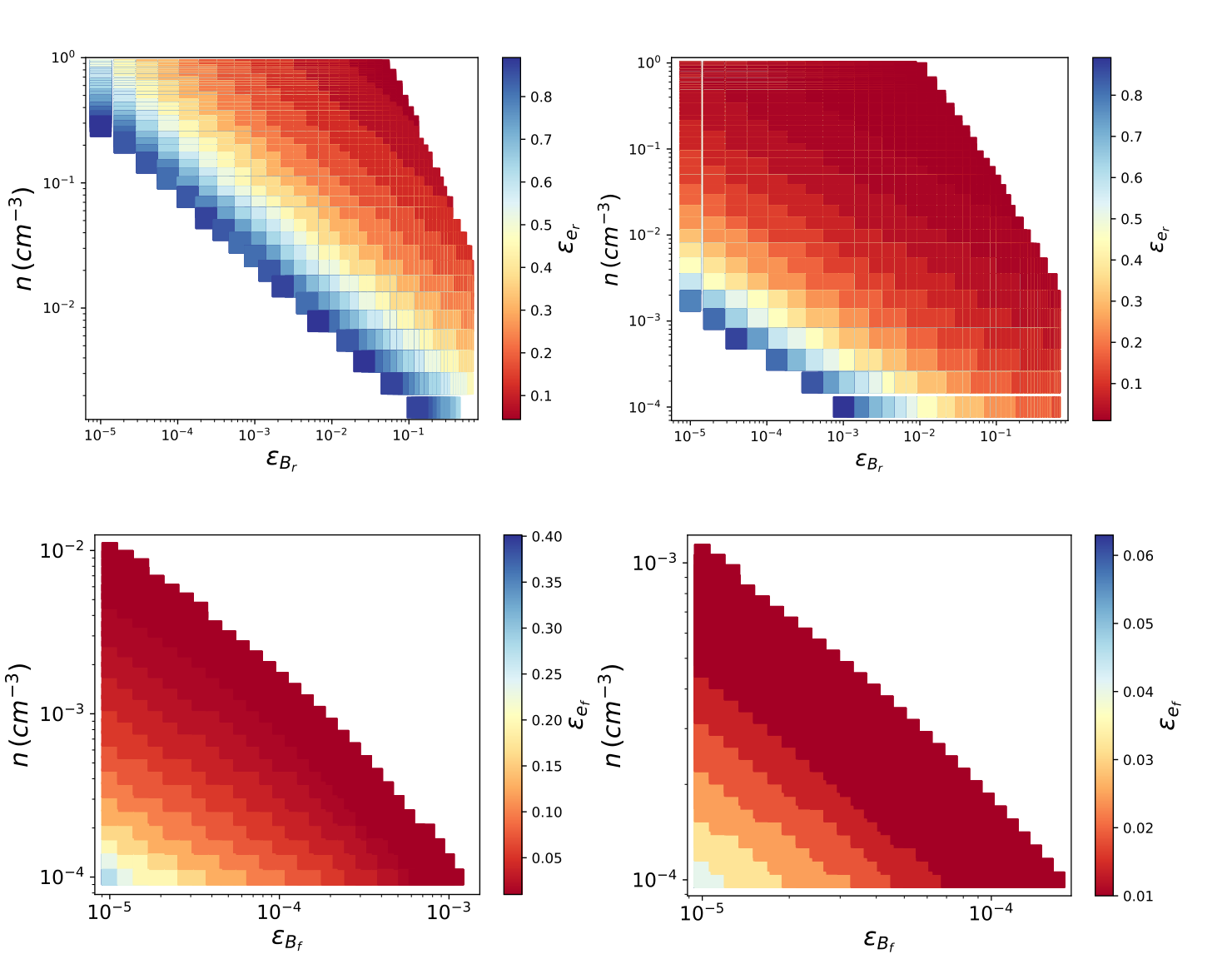
As an illustration, we show the parameter space of the microphysical parameters and the density of the circumburst medium for which (i) the RS SSC emission is in the thick-shell regime at 10 s, with a flux density mJy at 100 MeV (Figure 2, upper panels), and (ii) the FS cooling frequency, crosses 100 MeV between 100 and 500 s after the onset of the burst (Figure 2, lower panels), resulting in a break in the 100 MeV light curve. We explore two different values of the isotropic-equivalent kinetic energy, erg (left column) and erg (right column). The time interval of 100–500 s is chosen to explore the breaks observed in some bursts (Ajello et al. 2019, e.g. GRB 160509A;). The value of the threshold flux was estimated considering the sensitivity of Fermi-LAT reported by Piron 2016; De Angelis et al. 2017. It is worth noting that the parameter is quite strongly constrained from radio peaks in GRB afterglows (Beniamini and van der Horst 2017, e.g. see).
In the model with erg, there are no values of the physical parameters for which both a GeV flare RS SSC emission and a break in the FS synchrotron radiation due to the passage of are simultaneously observed, as long as and . In the model with erg, the two phenomena can be observed in the same burst provided the density is low, and if the RS region is highly magnetized, . Indeed, such large magnetizations are expected in magnetically dominated models for the GRB emission (Giannios 2008; Zhang and Yan 2011; McKinney and Uzdensky 2012; Beniamini and Piran 2014; Sironi 2015; Beniamini and Granot 2016; Bégué et al. 2017; Beniamini and Giannios 2017; Beniamini et al. 2018, e.g.,). Similarly, it can be inferred that the GeV flare in the LAT light curves is unlikely in a weak (e.g. low-luminosity) GRB, even in a low-density environment. Moderately high values of magnetization also have been inferred from several multi-wavelength RS studies, GRB 130427A (–5; Laskar et al. 2013; Perley et al. 2014), GRB 160509A (; Laskar et al. 2016a), GRB 160625B (–10; Alexander et al. 2017), although see also Laskar et al. 2019 for a system with detected by Fermi-LAT. We thus infer that the presence of simultaneous RS SSC emission and a break in the FS MeV light curve suggests a system with and/or a combination of high , a low-density environment, and strong relative magnetization between the RS and FS.
We now apply these principles to investigate the LAT light curve of GRB 160509A. Later on in Section 4, we provide high-energy light curve predictions in the thin-shell regime, using the example of GRB 180418A.
III. GRB 160509A: The thick-shell case
At 08:59:04.36 UTC on 2016 May 09, both instruments onboard Fermi satellite, GBM (Gamma Burst Monitor), and LAT triggered and located GRB 160509A (Roberts et al. 2016; Longo et al. 2016). The burst was located with coordinates and (J2000) with an error radius of (90% containment, the systematic error only). The LAT instrument detected a very energetic photon with an energy of 52 GeV, at s after the trigger. The GBM light curve in the 50 - 300 keV energy range exhibited multiple peaks with a duration of s. The Gemini North telescope observed this burst at 13:15 UT on 10 May 2016, obtaining optical spectroscopy and near-IR imaging with GMOS-N and NIRI instruments, respectively. A single and well-defined emission line ([OII] 3727 Å) in the spectroscopic analysis indicated a redshift of z=1.17 (Tanvir et al. 2016). In the radio bands, this burst was detected with the VLA (Very Large Array) at frequencies spanning between 1.3 and 37 GHz, beginning 0.36 days after the trigger time (Laskar et al. 2016b).
III.1. Fermi-LAT observations
The Fermi-LAT light curve of GRB 160509A66
6
LAT data points are taken from https://www-glast.stanford.edu/pub_data/953/. The energy range of 0.1 - 100 GeV integrated over the spectrum is used to convert from to at 100 MeV. exhibits two components: a GeV flare with a duration of 20 s and a long-lasting emission that begins 40 s after the LAT trigger and extends for more than s (Figure 3; red points). We fit the light curve with a series of broken PLs (next two sections) and discuss each component separately. The best-fit values of the GeV flare and the long-lasting emission are reported in Table 1. It is worth noting that in Ajello et al. 2019 the function defined by Willingale et al. 2007 was used to explore the existence of the plateau phase and to model it simultaneously with the prompt emission component. The best-fit values reported of the PL indices before and after the break time were and , respectively (Ajello et al. 2019, see Table 5 in). Thus, regardless of the function used, the presence of two components is visible.
III.1.1 The GeV flare
To describe the GeV flare, two PL functions were used: for and for . The term is the starting time of the GeV flare (Kobayashi and Zhang 2007; Vestrand et al. 2006), is the time for which the flux reaches the maximum value and begins decreasing, and and are the temporal rise and decay indexes, respectively. Using linear least squares (Lai et al. 1978) fitting implemented in ROOT, which is a modular, publicly available scientific software (Brun and Rademakers 1997), we found that the best-fit values are , and .
Maxham et al. 2011 investigated a FS origin for the GeV light curves of four GRBs (080916C, 090510, 090902B, and 090926A). They demonstrated that at , FS emission could explain the GeV light curve. However, the FS synchrotron contribution usually underpredicts the GeV light curve while the central engine is active (i.e., at ) due to the expectation of on-going energy accumulation in the FS over this period. We note that the GeV flare in GRB 160509A occurs at . We posit that a possible mechanism to reconcile the discrepancy noted by Maxham et al. 2011 may lie in RS SSC emission.
Comparing the best-fit value with the temporal indexes of the SSC light curves for (eq. 27), we notice that it is consistent with SSC model in the range for . Other PL segments in the SSC light curves would produce atypical values of . Given the spectral index when the SSC emission evolves in the range , after the shock crossing time the flux decays as (eq. 13) and finally due to high-latitude emission. Other PL segments of the SSC light curve cannot reproduce the decaying phase. Therefore, the best-fit parameters of the rise and decay PL indexes indicate that the GeV flare is consistent with a RS evolving in the uniform-density medium and the thick-shell regime.
The best-fit values of each component are reported in Table 1.
III.1.2 The long-lasting emission
The long-lasting emission component is described with a broken PL function of the form
| (35) |
The parameters and are the temporal indexes before and after the time break . We fit this model to the LAT light curve at using the chi-square method (Brun and Rademakers 1997). Our best-fit values are , and which are consistent with those reported in the second LAT GRB catalog (Ajello et al. 2019, see Fig. 27 in).
On the other hand, Tam et al. 2017 analyzed the LAT spectrum of the long-lasting emission. Using a PL function Tam et al. 2017 reported two distinct spectral indexes; for s and for s. Therefore, this component of the Fermi LAT observations can be described by before s and after s. In the synchrotron framework (section 2.2), the passage of the synchrotron cooling frequency is expected to result in the steepening of the light curve by , and a change in the spectral index by , both of which are consistent with the observed evolution in the LAT light curve and spectrum across . Furthermore, the sign of across the break is a diagnostic of the density profile. The steepening seen here is indicative of a uniform-density environment. This is also consistent with the inference of Laskar et al. 2016b, who infer a uniform-density environment based on modelling the RS emission at radio wavelengths for this burst. Taking at (where the data are less affected by potential contamination from the earlier GeV flare), we find . This yields , consistent with the observed value. Before the break, we expect a decay rate of and spectral slope of , consistent with observations. Therefore, the Fermi-LAT observations are consistent with a FS emission in a uniform-density environment, with the spectral ordering at s and at s, further implying that crosses the LAT band at s. The value of for the FS is also consistent with that previously obtained by Laskar et al. 2016b using the X-ray observations for this burst.
III.2. Constraint on the parameters from the afterglow observations
III.2.1 Afterglow observations
The Swift XRT (X-ray Telescope) followed-up GRB 160509A in a series of observations (seven) tiled on the sky (Kennea et al. 2016). The data in all modes began to be collected from s to 20 days after the trigger time. The XRT data used in this analysis is publicly available in the website database.77
7
http://www.swift.ac.uk/xrtproducts/ The XRT flux was extrapolated from 10 keV to 1 keV with the conversion factor shown in Evans et al. 2010. In the PC mode, the spectral value of the photon index was for a galactic (intrinsic) absorption of .
Laskar et al. 2016b analyzed the entire XRT data using the HEASOFT (v6.18) to fit the spectra. These authors initially using a broken PL and reported two spectral indexes of and for the intervals to and to , respectively. Supposing that the spectral index did not evolve during the whole interval, they used a PL and reported an X-ray spectral index of for the entire interval. It is worth noting that the values of the spectral index reported in the website database and by Laskar et al. 2016b are consistent.
Magenta data points in Figure 3 show the XRT light curve obtained at 1 keV.88
8
https://www.swift.ac.uk/burst_analyser/00020607/ In accordance with the shape of the X-ray light curve, it is divided in three intervals, labelled II (), III (), and IV (). We model each segment of the light curve with a PL function () using the chi-square minimization method. The best-fit indexes are , and , for the intervals II, III and IV, respectively. The best-fit value of each interval with its corresponding chi-square test statistic is reported in Table 2.
Using the closure relations, the flux during the interval III is described by , which can be understood as FS synchrotron emission in the regime, with . Given that the spectral index remains unchanged during the intervals II and IV, the interval II with the index is consistent with the plateau phase, while the steepening of the light curve in interval IV () is consistent with post-jet break evolution.
Our observation that at , together with our prior inference that at (Section 3.1.2), implies a rapid evolution of the FS synchrotron cooling frequency99 9 In fact, and are consistent within the error bars, which would suggest that the break in the X-ray light curve at s is due to the passage of . We verify this in section 3.3.1., at least as fast as . This is at variance with the expectation of in a uniform-density environment (Sari et al. 1998). Similar rapid evolution of has been inferred in other cases, with potential explanations involving time evolution of the microphysical parameters, steep circumburst density profiles, energy injection into the FS, and the proximity of the jet break (Racusin et al. 2008; Filgas et al. 2011; van Eerten and MacFadyen 2012).
Here, we consider the evolution of microphysical parameters (, ) as a possible explanation. The total energy transferred from protons to electrons and magnetic field is not well understood during the FS, so the fraction of electron and the magnetic density during the afterglow could vary (Yost et al. 2003; Kumar and Panaitescu 2003; Ioka et al. 2006; Fan and Piran 2006; Panaitescu et al. 2006, e.g., see). We emphasize that this is one possible model with the potential to explain the rapid evolution of . In this model, the synchrotron light curve in the slow cooling regime is given by
| (36) |
where the synchrotron spectral breaks evolve as and . It is worth noting that once the microphysical parameters stop evolving (i.e., and ), the standard synchrotron FS model is recovered (Sari et al. 1998).
To summarize, the LAT light curve at s is consistent with SSC emission from a RS in the thick-shell regime and a uniform-density circumburst environment. The LAT data at s and the X-ray light curve are consistent with synchrotron emission from the FS in a uniform-density circumburst environment with and the spectral ordering for and for .
III.2.2 Constraint on the parameters
We normalize the synchrotron emission at 100 MeV and 1 keV for the LAT and X-ray observations, respectively. The synchrotron light curves that evolve in a uniform-density medium before (Sari et al. 1998) and after (Sari et al. 1999) the jet break were used to describe the long-lasting LAT and X-ray emissions, and the GeV flare observed before 40 s are fitted with the SSC emission in the thick-shell regime (eqs. 12 and 19). The synchrotron FS model with varying the microphysical parameters is used to describe the X-ray flux during the time interval - s (eq. 36). The luminosity distance was estimated using the cosmological parameters reported in Planck Collaboration et al. 2018. Using our estimate of and the isotropic-equivalent -ray energy, erg (Ajello et al. 2019), we obtain a prompt gamma-ray efficiency of .
Our analytical afterglow model, as described in Section II, is completely determined by a set of nine parameters . We, then, assign prior distributions to these parameters for application in a Markov-Chan Monte Carlo (MCMC) simulation. Shape-wise we choose Normal distributions for each physical parameter of the system; this allows us to pass the minimum amount of information (and consequently bias) necessary for the simulation. After determining the shape, we then assign a mean and standard deviation for each parameter. The choice of values is such that our prior distributions cover a range of the typical values found for these parameters in the literature of GRB afterglow modelling (Kumar and Barniol Duran 2009; Kumar and Zhang 2015; Ajello et al. 2019, e.g, see), while maintaining a reasonable computational time. We then assign a likelihood function described by a Normal distribution whose mean is our afterglow model and standard deviation is a hyperparameter . For this hyperparameter we chose a value that returns a distribution sufficiently large so that the likelihood can explore the region around the detections containing the data uncertainty, similarly to the models we used in Fraija et al. 2019d. We opted to use a Half-Normal distribution, with static standard deviation, to describe this parameter, this way our likelihood is allowed to better explore the space around the observed data giving more leeway to the sampler. We use the No-U-TurnSampler from the PyMC3 python distribution to generate a total of 17300 samples, allowing a total of 7000 tuning iterations. The results of the MCMC analysis are summarized in Table 3. The best-fitting curves are shown in Figure 3. The corner plot displaying the one-dimensional marginalized posterior distributions for each parameter and the two-dimensional marginalized posterior distributions for each pair of parameters is shown in Figure 4. It is worth nothing that a Bayesian technique of checking the ability of the model to explain the observed data are posterior predictive checks (Gabry et al. 2019). Concerns about the convergence of affine invariant ensemble sampler in high dimension are described by Huijser et al. 2015. We use the Gelman and Rubin’s convergence diagnostic (Gelman and Rubin 1992) through the parameter for each variable verify the convergence of the sampler. For all variables the returned values , indicating a well-behaved, converging sampler.
Based on the values reported in Table 3, the implications of the results are discussed in the following section.
III.3. Implications of the Results and Discussion
III.3.1 Microphysical parameters
Given the microphysical parameter associated with the magnetic field in the RS region (), the magnetization parameter (Zhang and Kobayashi 2005, see Fig. 6 in) lies in the range which corresponds to a regime for which the RS is produced. In the RS region, the self-absorption, the characteristic, and the cutoff frequency breaks of synchrotron radiation at 30 s are , and , respectively. It shows that the synchrotron emission evolves in the slow-cooling regime and lies in the weak self-absorption regime so that a thermal component is not expected by this mechanism (Kobayashi and Zhang 2003).
The best-fit values of the magnetic field parameters from the FS and RS regions are different. The evolution of the RS requires that the outflow is moderately magnetized .1010 10 Laskar et al. 2016b reported a value of .
In the radio bands, Laskar et al. 2016b presented a multi-frequency radio detection with the VLA beginning 0.36 days after the trigger time. The VLA observations were carried out at frequencies spanning 1.3 and 37 GHz. These authors found that the X-ray and radio emission originated from distinct regions. They modelled the radio to X-ray emission as a combination of synchrotron radiation from both the RS and FS. They showed that the radio observations were dominated up to 10.03 days by synchrotron from the RS region. Our best-fit values using LAT and X-ray observations, , , and are consistent with the values of Laskar et al. 2016b, who found , , and . Our values of the FS microphysical parameters ( and ) are much smaller than reported by Laskar et al. 2016b ( and ); however, we note that both sets of analyses suffer from some degeneracy, since (i) the observations do not allow us to locate the FS synchrotron self-absorption break, and (ii) is not uniquely constrained due to the large optical extinction along the line of sight. Thus, it is possible that the true values of these parameters are intermediate between those derived here and in Laskar et al. 2016b.
During the plateau phase ( s) the microphysical parameters are given by and with the best-fit values of and for a normalization time fixed to . While the magnetic parameter increases with time, the electron density parameter decreases. It is worth noting that different authors have considered distinct possibilities in the evolution of the microphysical parameters (Fan and Piran 2006; Panaitescu et al. 2006; Kumar and
Panaitescu 2003; Ioka et al. 2006, e.g., see). With the best-fit values, the synchrotron break frequencies evolves as and , and the flux as for . One can see that the best-fit value of the temporal index in the interval II (the plateau phase) reported in Table 2 agrees with the predicted value of derived when the microphysical parameters evolve with time. Similarly, the rapid evolution of indicates that the breaks observed in the LAT and the X-ray light curve at s and , respectively, can be interpreted as the passage of the synchrotron cooling break through the Fermi-LAT and Swift-XRT bands at 100 MeV and 1 keV, respectively.
III.3.2 The bulk Lorentz factors
Our analysis of the multi-wavelength afterglow observations leads to an initial bulk and critical Lorentz factors of 600 and , respectively.1111
11
The bulk Lorentz factor is obtained using eq. 2 and the best-fit values reported in Table 3. As expected the bulk Lorentz factor is above the critical one. This shows our RS model evolving in the thick-shell regime is self-consistent.
The break observed in the X-ray observations at s is associated with a jet break. This value leads to a jet opening angle of and a bulk Lorentz factor at the jet-break time of = 6.9 (Sari et al. 1999). The jet opening angle obtained is twice the value reported in Laskar et al. 2016b, so their result is not based solely on the X-ray light curve
The value of the initial bulk Lorentz factor inferred during the deceleration phase is similar to those reported by other burst detected by Fermi-LAT (Veres and
Mészáros 2012). Since GRB 160509A exhibited one of the most energetic photons reported by Fermi-LAT in the second GRB catalog, it is expected that the value of the bulk Lorentz factor lies in the range of the brightest LAT-detected bursts (Ackermann et al. 2011; Ackermann and
et al. 2013; Abdo et al. 2009a; Ackermann and
et al. 2010; Ackermann et al. 2014; Fraija et al. 2019b; Fraija et al. 2019c, ;), as found in this work.
III.3.3 The ambient density profile
If we consider the core-collapse scenario for long GRBs (Woosley 1993; MacFadyen and Woosley 1999; Woosley and Bloom 2006, e.g.) then stellar winds from the massive star are expected to form the circumburst medium which scale as a function of the radius (Chevalier and Li 1999, e.g.). Beyond the wind termination shock, the density profile is expected to transition from a wind-like to the uniform-density interstellar medium (Fraija et al. 2017).
Tak et al. 2019 analyzed 26 long bright GRBs and showed that a subset of these events (22 GRBs) could be explained with the uniform-density medium. Other observational studies reached similar conclusions (Yost et al. 2003; Schulze et al. 2011, e.g.,). These outcomes may imply that a wind profile cannot be explained when the radii of the FS is reached (Schulze et al. 2011).
The best-fit value of the circumburst density indicates that GRB 160509A exploded in an environment with very low density comparable to a halo or intergalactic medium with . The inferred low density agrees with our prediction (Section 2.3) that the simultaneous occurrence of a GeV flare and a late-time break in the LAT light curve (due to the passage of ) requires cm-3 for typical parameters. A large fraction (22) of LAT-detected GRBs have been shown to have exploded in an environment best described as a uniform-density medium (Tak et al. 2019), and GRB 160509A continues this trend.
Although Laskar et al. 2016b favored a uniform-density environment for this burst on physical grounds (based on the inferred initial Lorentz factor from the RS emission), they could not conclusively distinguish between a wind a uniform-density medium based on X-ray, optical, and radio afterglow observations alone. As shown in this paper, the analysis of the LAT observations suggests that this is consistent with the evolution of the external shocks in a uniform-density medium.
III.3.4 VHE photons above synchrotron limit and SSC emission from FS
Ajello et al. 2019 presented in the second Fermi-LAT GRB catalog the bursts with photon energies above 10 GeV. Two such photons were associated with GRB 160509A, the first photon with an energy of 51.9 GeV arriving at 76.5 s and the second one of 41.5 GeV arriving at 242 s after the trigger time. Given the best-fit parameters (see Table 3), the maximum energy photons produced by synchrotron radiation during the evolution of the FS are 6.82 and 4.43 GeV at 76.5 and 242 s, respectively.1212
12
We use the upper limit on the energy of photons that can be produced by synchrotron radiation in FSs (Kumar and Barniol
Duran 2009; Fraija et al. 2019a, e.g., see). Furthermore, RS SSC emission cannot explain the highest-energy photons detected at 76.5 s and 242 s after the trigger time because this component is subdominant to the synchrotron FS emission at s. Therefore, the observed high-energy photons require a process distinct from both FS synchrotron and RS SSC emission. We now consider whether SSC emission from the FS could explain these photons (Beniamini et al. 2015; Fraija et al. 2019a, e.g., see).
Following Fraija et al. 2019a and the parameters reported for this burst (see Table 3), the spectral breaks and the maximum flux for SSC emission in the FS can be expressed as
| (37) | |||||
| (39) | |||||
| (41) | |||||
where is the Compton parameter for the FS (Wang et al. 2010; Beniamini et al. 2015; Fraija et al. 2019a). In the slow-cooling regime the SSC light curve is given by (Fraija et al. 2019a, e.g)
| (42) |
where and correspond to the energy band and timescale of this process, and the coefficients are given by
| (43) | |||||
| (45) | |||||
| (47) | |||||
Given eqs. (37) and (42), the two energetic photons at 76.5 s and 242 s associated with GRB 160509A lie in the range of . In this case, the number of VHE photons () arriving to LAT effective area () at 100 s can be estimated as which is consistent with observations. The conversion from normalized at to in the (0.1 - 100) GeV energy range for an spectral index of 2 is used.
Taking into account the distance to GRB 160509A, the SSC flux must be corrected by the extragalactic background light (EBL) attenuation. Using the model proposed in Franceschini and Rodighiero 2017, the attenuation factor at and is 0.5.
The frequency above which KN effects are important can be written as
| (49) | |||||
which is above the energy range considered. Given the minimum () and cooling () electron Lorentz factors shown in Fraija et al. 2019a, the synchrotron and SSC luminosity ratio can be computed as (Sari and Esin 2001)
| (50) |
where is the FS radius. In the case of a uniform medium, 70% of the synchrotron luminosity is up-scattered by SSC emission. The KN suppression for the SSC photon is important above .
The HAWC observatory performed a search for VHE (0.1 - 100 TeV) photons in temporal (using four search windows) and spatial coincidence with GRB 160509A (Lennarz and
Taboada 2016). One of these time windows corresponds to around the time (from - 20 to 20 s) of the highest-energy photon reported by LAT 77 s after the trigger time. In all the time windows including around the highest-energy photon were consistent with background only.
At the trigger time reported by Fermi-LAT, GRB 160509A was at an elevation of and culminated at inside the HAWC’s field of view (Lennarz and
Taboada 2016). Taking into account the sensitivity of HAWC to GRBs described in Abeysekara et al. 2012 for a range of the zenith angle between , an upper limit at and a spectral index of could be derived as . In this case, the theoretical flux predicted through eq. (42) is , which agrees with the upper limit derived.
IV. Predicted Light Curve of GRB 180418A: Thin-shell case
At 06:44:06.012 UTC on 18 April 2018, the Swift BAT instrument triggered and located GRB 180418A (D’Elia et al. 2018). The BAT light curve in the energy range of 15 -150 keV exhibited a single FRED-like pulse with a duration of . At 06:44:06.28 UTC on 18 April 2018, Fermi GBM triggered on GRB 180418A (Bissaldi and
Veres 2018). The light curve consisted of a single FRED-like peak similar to the BAT light curve, with a duration of , and a fluence of measured in the energy range of 10-1000 keV. The Fermi-LAT instrument did not detect GRB 180418A. Because of an observing constraint, the Swift XRT and UVOT instruments could not begin observing this burst until 3081.4 s and 3086 s after the trigger time, respectively. The TAROT and RATIR optical telescopes started observing GRB 180418A in several filters 28.0 and 120.6 s after the trigger time, respectively (Becerra et al. 2019).
Becerra et al. 2019 presented observations of GRB 180418A in -ray, X-ray, and optical bands suggesting that this burst may have been a sGRB. This burst exhibited a bright optical flare (Becerra et al. 2019, AB mag in the r band;) peaking between 28 and 90 s after the trigger time. The early optical observations were interpreted as synchrotron RS model in the thin-shell regime and in a uniform-density medium for . Taking into account the isotropic-equivalent kinetic energy of and a redshift of , the values of the parameters found by Becerra et al. 2019 are: the circumburst density (), the bulk Lorentz factor () and the microphysical parameters ( and ).
Using eqs. (25) and (34) and the parameters reported by Becerra et al. 2019, we plot the theoretically predicted SSC emission from the RS evolving in the thin-shell regime and the Fermi-LAT sensitivity extrapolated at 1 GeV, as shown in Figure 5. This figure shows the X-ray and optical observations with the best-fit curve for synchrotron RS emission1313 13 The derived quantities as the synchrotron break frequencies, fluxes and the evolution of the Lorentz factor are reported in Becerra et al. 2019. and the predicted SSC emission.1414 14 The optical peak is well separated from the prompt emission, which is a hallmark of the thin-shell model. It shows that the SSC emission is around two orders of magnitude below the Fermi-LAT sensitivity, which agrees with the non-detections reported by this instrument.
V. Summary
We have derived the SSC light curves from RS in thick- and thin-shell regimes for a uniform-density medium and shown that this emission in the thick-shell case could describe the GeV flares exhibited in some interesting LAT-detected bursts (Ghisellini et al. 2010; Lü et al. 2017). Since the shock crossing time is less than the prompt emission in the thick-shell regime, a bright RS SSC peak is expected at the beginning of the FS emission. By contrast, as the shock crossing time is longer than the duration of the prompt emission in the thin-shell regime, a bright RS SSC peak, in this case, appears distinct from the prompt emission and can be expected during the FS emission. The rise and decay indices of the RS SSC light curves are expected to be and for a thick-shell regime, and and for a thin-shell regime, respectively. We have shown that a bright RS SSC peak is expected when the microphysical parameter is above 0.1 and suppressed when .
We have also investigated the nature of late-time breaks in GeV light curves, and interpret these as the passage of the synchrotron cooling frequency of the FS through the GeV band. This naturally occurs in a uniform, low-density environment. For
more energetic bursts, a lower density is needed for this effect to be observed. We have shown that the simultaneous presence of GeV flare and a break in the LAT light curve requires a low density and , suggesting that the outflow could be endowed with primordial magnetic fields in such cases.
We emphasize that the FS closure relations are not expected to be satisfied when the LAT light curves are a superposition of SSC and synchrotron from RS and FS, respectively. Only when the RS SSC emission is suppressed or has decreased sufficiently so that it is negligible regarding the synchrotron FS emission, the closure relation can be satisfied in the LAT energy band. It is worth highlighting that, depending on the parameter values, GeV flare RS SSC emission could be hidden by longer-lasting FS synchrotron emission.
As a particular case for the thick-shell regime, we have studied the LAT observations of GRB 160509A, which exhibited a clear, bright peak at 20 s with a break at 316 s in the light curve. With the values of the best-fit parameters, we inferred that the first photon with an energy of 51.9 GeV arriving at 76.5 s and the second one of 41.5 GeV arriving at 242 s after the trigger time is produced in the deceleration phase of the outflow and a different mechanism to the standard synchrotron model has to be invoked to interpret these VHE photons. We explicitly showed that the SSC FS emission generates these VHE photons. The best-fit values of the microphysical parameters indicate that a magnetized outflow could explain the features exhibited in the light curves of GRB 160509A.
As an example of the thin-shell regime, we have predicted the light curves at 100 MeV for GRB 180418A with the parameters used to describe the X-ray and optical observations. As expected, the light curves at 100 MeV are below the Fermi-LAT sensitivity.
References
- Abdo et al. (2009a) Abdo, A. A., Ackermann, M., Ajello, M., Asano, K., Atwood, W. B., Axelsson, M., Baldini, L., Ballet, J., Barbiellini, G., Baring, M. G., Bastieri, D., Bechtol, K., Bellazzini, R., and et al (2009a). Fermi Observations of GRB 090902B: A Distinct Spectral Component in the Prompt and Delayed Emission. ApJ, 706:L138–L144.
- Abdo et al. (2009b) Abdo, A. A., Ackermann, M., Arimoto, M., Asano, K., Atwood, W. B., Axelsson, M., Baldini, L., Ballet, J., Band, D. L., Barbiellini, G., and et al. (2009b). Fermi Observations of High-Energy Gamma-Ray Emission from GRB 080916C. Science, 323:1688.
- Abeysekara et al. (2012) Abeysekara, A. U., Aguilar, J. A., Aguilar, S., Alfaro, R., Almaraz, E., Álvarez, C., and et al. (2012). On the sensitivity of the HAWC observatory to gamma-ray bursts. Astroparticle Physics, 35:641–650.
- Ackermann et al. (2014) Ackermann, M., Ajello, M., Asano, K., Atwood, W. B., Axelsson, M., Baldini, L., Ballet, J., Barbiellini, G., Baring, M. G., and et al. (2014). Fermi-LAT Observations of the Gamma-Ray Burst GRB 130427A. Science, 343:42–47.
- Ackermann et al. (2011) Ackermann, M., Ajello, M., Asano, K., Axelsson, M., Baldini, L., Ballet, J., Barbiellini, G., Baring, M. G., Bastieri, D., Bechtol, K., and et al (2011). Detection of a Spectral Break in the Extra Hard Component of GRB 090926A. ApJ, 729:114.
- Ackermann and et al. (2010) Ackermann, M. and et al. (2010). Fermi Observations of GRB 090510: A Short-Hard Gamma-ray Burst with an Additional, Hard Power-law Component from 10 keV TO GeV Energies. ApJ, 716:1178–1190.
- Ackermann and et al. (2013) Ackermann, M. and et al. (2013). Multiwavelength Observations of GRB 110731A: GeV Emission from Onset to Afterglow. ApJ, 763:71.
- Ajello et al. (2019) Ajello, M., Arimoto, M., Axelsson, M., Baldini, L., Barbiellini, G., Bastieri, D., and et al. (2019). A decade of gamma-ray bursts observed by fermi-LAT: The second GRB catalog. The Astrophysical Journal, 878(1):52.
- Alexander et al. (2017) Alexander, K. D., Laskar, T., Berger, E., Guidorzi, C., Dichiara, S., Fong, W., and et al. (2017). A Reverse Shock and Unusual Radio Properties in GRB 160625B. ApJ, 848(1):69.
- Ayache et al. (2020) Ayache, E. H., van Eerten, H. J., and Daigne, F. (2020). Late X-ray flares from the interaction of a reverse shock with a stratified ejecta in GRB afterglows: simulations on a moving mesh. arXiv e-prints, page arXiv:2004.04179.
- Becerra et al. (2019) Becerra, R. L., Dichiara, S., Watson, A. M., Troja, E., Fraija, N., Klotz, A., Butler, N. R., Lee, W. H., Veres, P., Turpin, D., Bloom, J. S., Boer, M., González, J. J., Kutyrev, A. S., Prochaska, J. X., Ramirez-Ruiz, E., and Richer, M. G. (2019). Reverse Shock Emission Revealed in Early Photometry in the Candidate Short GRB 180418A. ApJ, 881(1):12.
- Bégué et al. (2017) Bégué, D., Pe’er, A., and Lyubarsky, Y. (2017). Radiative striped wind model for gamma-ray bursts. MNRAS, 467(3):2594–2611.
- Beniamini et al. (2018) Beniamini, P., Barniol Duran, R., and Giannios, D. (2018). Marginally fast cooling synchrotron models for prompt GRBs. MNRAS, 476(2):1785–1795.
- Beniamini and Giannios (2017) Beniamini, P. and Giannios, D. (2017). Prompt gamma-ray burst emission from gradual magnetic dissipation. MNRAS, 468(3):3202–3211.
- Beniamini and Granot (2016) Beniamini, P. and Granot, J. (2016). Properties of GRB light curves from magnetic reconnection. MNRAS, 459(4):3635–3658.
- Beniamini et al. (2015) Beniamini, P., Nava, L., Duran, R. B., and Piran, T. (2015). Energies of GRB blast waves and prompt efficiencies as implied by modelling of X-ray and GeV afterglows. MNRAS, 454:1073–1085.
- Beniamini and Piran (2014) Beniamini, P. and Piran, T. (2014). The emission mechanism in magnetically dominated gamma-ray burst outflows. MNRAS, 445:3892–3907.
- Beniamini and van der Horst (2017) Beniamini, P. and van der Horst, A. J. (2017). Electrons’ energy in GRB afterglows implied by radio peaks. MNRAS, 472(3):3161–3168.
- Bissaldi and Veres (2018) Bissaldi, E. and Veres, P. (2018). GRB 180418A: Fermi GBM observation. GRB Coordinates Network, 22656:1.
- Brun and Rademakers (1997) Brun, R. and Rademakers, F. (1997). ROOT - An object oriented data analysis framework. Nuclear Instruments and Methods in Physics Research A, 389:81–86.
- Cavallo and Rees (1978) Cavallo, G. and Rees, M. J. (1978). A qualitative study of cosmic fireballs and gamma -ray bursts. MNRAS, 183:359–365.
- Chevalier and Li (1999) Chevalier, R. A. and Li, Z.-Y. (1999). Gamma-Ray Burst Environments and Progenitors. ApJ, 520:L29–L32.
- Dainotti et al. (2011) Dainotti, M. G., Ostrowski, M., and Willingale, R. (2011). Towards a standard gamma-ray burst: tight correlations between the prompt and the afterglow plateau phase emission. MNRAS, 418(4):2202–2206.
- De Angelis et al. (2017) De Angelis, A., Tatischeff, V., Tavani, M., Oberlack, U., Grenier, I., Hanlon, L., and et al. (2017). The e-ASTROGAM mission. Exploring the extreme Universe with gamma rays in the MeV - GeV range. Experimental Astronomy, 44(1):25–82.
- D’Elia et al. (2018) D’Elia, V., D’Ai, A., Evans, P. A., Page, K. L., Palmer, D. M., Sbarufatti, B., Stamatikos, M., and Tohuvavohu, A. (2018). GRB 180418A: Swift detection of a short burst. GRB Coordinates Network, 22646:1.
- Evans et al. (2010) Evans, P. A., Willingale, R., Osborne, J. P., O’Brien, P. T., Page, K. L., Markwardt, C. B., Barthelmy, S. D., Beardmore, A. P., Burrows, D. N., Pagani, C., Starling, R. L. C., Gehrels, N., and Romano, P. (2010). The Swift Burst Analyser. I. BAT and XRT spectral and flux evolution of gamma ray bursts. A&A, 519:A102.
- Fan and Piran (2006) Fan, Y. and Piran, T. (2006). Gamma-ray burst efficiency and possible physical processes shaping the early afterglow. MNRAS, 369(1):197–206.
- Filgas et al. (2011) Filgas, R., Greiner, J., Schady, P., Krühler, T., Updike, A. C., Klose, S., and et al. (2011). GRB 091127: The cooling break race on magnetic fuel. A&A, 535:A57.
- Fraija (2015) Fraija, N. (2015). GRB 110731A: Early Afterglow in Stellar Wind Powered By a Magnetized Outflow. ApJ, 804:105.
- Fraija et al. (2019a) Fraija, N., Barniol Duran, R., Dichiara, S., and Beniamini, P. (2019a). Synchrotron Self-Compton as a Likely Mechanism of Photons beyond the Synchrotron Limit in GRB 190114C. ApJ, 883(2):162.
- Fraija et al. (2019b) Fraija, N., Dichiara, S., Pedreira, A. C. C. d. E. S., Galvan-Gamez, A., Becerra, R. L., Barniol Duran, R., and Zhang, B. B. (2019b). Analysis and Modeling of the Multi-wavelength Observations of the Luminous GRB 190114C. ApJ, 879(2):L26.
- Fraija et al. (2019c) Fraija, N., Dichiara, S., Pedreira, A. C. C. d. E. S., Galvan-Gamez, A., Becerra, R. L., Montalvo, A., Montero, J., Betancourt Kamenetskaia, B., and Zhang, B. B. (2019c). Modeling the Observations of GRB 180720B: from Radio to Sub-TeV Gamma-Rays. ApJ, 885(1):29.
- Fraija et al. (2016a) Fraija, N., Lee, W., and Veres, P. (2016a). Modeling the Early Multiwavelength Emission in GRB130427A. ApJ, 818:190.
- Fraija et al. (2016b) Fraija, N., Lee, W. H., Veres, P., and Barniol Duran, R. (2016b). Modeling the Early Afterglow in the Short and Hard GRB 090510. ApJ, 831:22.
- Fraija et al. (2019d) Fraija, N., Pedreira, A. C. C. d. E. S., and Veres, P. (2019d). Light Curves of a Shock-breakout Material and a Relativistic Off-axis Jet from a Binary Neutron Star System. ApJ, 871:200.
- Fraija and Veres (2018) Fraija, N. and Veres, P. (2018). The Origin of the Optical Flashes: The Case Study of GRB 080319B and GRB 130427A. ApJ, 859:70.
- Fraija et al. (2017) Fraija, N., Veres, P., Zhang, B. B., Barniol Duran, R., Becerra, R. L., Zhang, B., Lee, W. H., Watson, A. M., Ordaz-Salazar, C., and Galvan-Gamez, A. (2017). Theoretical Description of GRB 160625B with Wind-to-ISM Transition and Implications for a Magnetized Outflow. ApJ, 848:15.
- Franceschini and Rodighiero (2017) Franceschini, A. and Rodighiero, G. (2017). The extragalactic background light revisited and the cosmic photon- photon opacity. A&A, 603:A34.
- Gabry et al. (2019) Gabry, J., Simpson, D., Vehtari, A., Betancourt, M., and Gelman, A. (2019). Visualization in bayesian workflow. JOURNAL OF THE ROYAL STATISTICAL SOCIETY SERIES A: STATISTICS IN SOCIETY, 182(2):389–402.
- Gelman and Rubin (1992) Gelman, A. and Rubin, D. B. (1992). Inference from Iterative Simulation Using Multiple Sequences. Statistical Science, 7:457–472.
- Ghisellini et al. (2010) Ghisellini, G., Ghirlanda, G., Nava, L., and Celotti, A. (2010). GeV emission from gamma-ray bursts: a radiative fireball? MNRAS, 403:926–937.
- Giannios (2008) Giannios, D. (2008). Prompt GRB emission from gradual energy dissipation. A&A, 480(2):305–312.
- Huijser et al. (2015) Huijser, D., Goodman, J., and Brewer, B. J. (2015). Properties of the Affine Invariant Ensemble Sampler in high dimensions. arXiv e-prints, page arXiv:1509.02230.
- Ioka et al. (2006) Ioka, K., Toma, K., Yamazaki, R., and Nakamura, T. (2006). Efficiency crisis of swift gamma-ray bursts with shallow X-ray afterglows: prior activity or time-dependent microphysics? A&A, 458(1):7–12.
- Kennea et al. (2016) Kennea, J. A., Roegiers, T. G. R., Osborne, J. P., Page, K. L., Melandri, A., D’Avanzo, P., D’Elia, V., Burrows, D. N., McCauley, L. M., Pagani, C., and Evans, P. A. (2016). GRB 160509A: Swift-XRT afterglow detection. GRB Coordinates Network, Circular Service, No. 19408, #1 (2016), 19408.
- Kobayashi (2000) Kobayashi, S. (2000). Light Curves of Gamma-Ray Burst Optical Flashes. ApJ, 545:807–812.
- Kobayashi and Sari (2000) Kobayashi, S. and Sari, R. (2000). Optical Flashes and Radio Flares in Gamma-Ray Burst Afterglow: Numerical Study. ApJ, 542(2):819–828.
- Kobayashi and Zhang (2003) Kobayashi, S. and Zhang, B. (2003). Early Optical Afterglows from Wind-Type Gamma-Ray Bursts. ApJ, 597:455–458.
- Kobayashi and Zhang (2007) Kobayashi, S. and Zhang, B. (2007). The Onset of Gamma-Ray Burst Afterglow. ApJ, 655:973–979.
- Kobayashi et al. (2007) Kobayashi, S., Zhang, B., Mészáros, P., and Burrows, D. (2007). Inverse Compton X-Ray Flare from Gamma-Ray Burst Reverse Shock. ApJ, 655:391–395.
- Kumar and Barniol Duran (2009) Kumar, P. and Barniol Duran, R. (2009). On the generation of high-energy photons detected by the Fermi Satellite from gamma-ray bursts. MNRAS, 400:L75–L79.
- Kumar and Barniol Duran (2010) Kumar, P. and Barniol Duran, R. (2010). External forward shock origin of high-energy emission for three gamma-ray bursts detected by Fermi. MNRAS, 409:226–236.
- Kumar and Panaitescu (2000) Kumar, P. and Panaitescu, A. (2000). Afterglow Emission from Naked Gamma-Ray Bursts. ApJ, 541:L51–L54.
- Kumar and Panaitescu (2003) Kumar, P. and Panaitescu, A. (2003). A unified treatment of the gamma-ray burst 021211 and its afterglow. MNRAS, 346:905–914.
- Kumar and Zhang (2015) Kumar, P. and Zhang, B. (2015). The physics of gamma-ray bursts relativistic jets. Phys. Rep., 561:1–109.
- Lai et al. (1978) Lai, T. L., Robbins, H., and Wei, C. Z. (1978). Strong consistency of least squares estimates in multiple regression. Proceedings of the National Academy of Sciences, 75(7):3034–3036.
- Laskar et al. (2016a) Laskar, T., Alexander, K. D., Berger, E., Fong, W.-f., Margutti, R., Shivvers, I., and et al. (2016a). A Reverse Shock in GRB 160509A. ApJ, 833(1):88.
- Laskar et al. (2016b) Laskar, T., Alexander, K. D., Berger, E., Fong, W.-f., Margutti, R., Shivvers, I., Williams, P. K. G., Kopač, D., Kobayashi, S., Mundell, C., Gomboc, A., Zheng, W., Menten, K. M., Graham, M. L., and Filippenko, A. V. (2016b). A Reverse Shock in GRB 160509A. ApJ, 833(1):88.
- Laskar et al. (2013) Laskar, T., Berger, E., Zauderer, B. A., Margutti, R., Soderberg, A. M., Chakraborti, S., Lunnan, R., Chornock, R., Chandra, P., and Ray, A. (2013). A Reverse Shock in GRB 130427A. ApJ, 776(2):119.
- Laskar et al. (2019) Laskar, T., van Eerten, H., Schady, P., Mundell, C. G., Alexander, K. D., Barniol Duran, R., Berger, E., Bolmer, J., Chornock, R., Coppejans, D. L., Fong, W.-f., Gomboc, A., Jordana-Mitjans, N., Kobayashi, S., Margutti, R., Menten, K. M., Sari, R., Yamazaki, R., Lipunov, V. M., Gorbovskoy, E., Kornilov, V. G., Tyurina, N., Zimnukhov, D., Podesta, R., Levato, H., Buckley, D. A. H., Tlatov, A., Rebolo, R., and Serra-Ricart, M. (2019). A Reverse Shock in GRB 181201A. ApJ, 884(2):121.
- Lennarz and Taboada (2016) Lennarz, D. and Taboada, I. (2016). GRB 160509A: non-observation of VHE emission with HAWC. GRB Coordinates Network, Circular Service, No. 19423, #1 (2016), 19423.
- Longo et al. (2016) Longo, F., Bissaldi, E., Bregeon, J., McEnery, J., Ohno, M., and Zhu, S. (2016). GRB 160509A: Fermi-LAT prompt detection of a very bright burst. GRB Coordinates Network, Circular Service, No. 19403, #1 (2016), 19403.
- Lü et al. (2017) Lü, H., Wang, X., Lu, R., Lan, L., Gao, H., Liang, E., Graham, M. L., Zheng, W., Filippenko, A. V., and Zhang, B. (2017). A Peculiar GRB 110731A: Lorentz Factor, Jet Composition, Central Engine, and Progenitor. ApJ, 843(2):114.
- MacFadyen and Woosley (1999) MacFadyen, A. I. and Woosley, S. E. (1999). Collapsars: Gamma-Ray Bursts and Explosions in “Failed Supernovae”. ApJ, 524(1):262–289.
- Maxham et al. (2011) Maxham, A., Zhang, B.-B., and Zhang, B. (2011). Is GeV emission from Gamma-Ray Bursts of external shock origin? MNRAS, 415:77–82.
- McKinney and Uzdensky (2012) McKinney, J. C. and Uzdensky, D. A. (2012). A reconnection switch to trigger gamma-ray burst jet dissipation. MNRAS, 419(1):573–607.
- Mészáros and Rees (1997) Mészáros, P. and Rees, M. J. (1997). Optical and Long-Wavelength Afterglow from Gamma-Ray Bursts. ApJ, 476:232–237.
- Nousek et al. (2006) Nousek, J. A., Kouveliotou, C., Grupe, D., Page, K. L., Granot, J., Ramirez-Ruiz, E., Patel, S. K., Burrows, D. N., Mangano, V., Barthelmy, S., Beardmore, A. P., Campana, S., Capalbi, M., Chincarini, G., Cusumano, G., Falcone, A. D., Gehrels, N., Giommi, P., Goad, M. R., Godet, O., Hurkett, C. P., Kennea, J. A., Moretti, A., O’Brien, P. T., Osborne, J. P., Romano, P., Tagliaferri, G., and Wells, A. A. (2006). Evidence for a Canonical Gamma-Ray Burst Afterglow Light Curve in the Swift XRT Data. ApJ, 642:389–400.
- Panaitescu and Kumar (2000) Panaitescu, A. and Kumar, P. (2000). Analytic Light Curves of Gamma-Ray Burst Afterglows: Homogeneous versus Wind External Media. ApJ, 543:66–76.
- Panaitescu et al. (2006) Panaitescu, A., Mészáros, P., Burrows, D., Nousek, J., Gehrels, N., O’Brien, P., and Willingale, R. (2006). Evidence for chromatic X-ray light-curve breaks in Swift gamma-ray burst afterglows and their theoretical implications. MNRAS, 369(4):2059–2064.
- Panaitescu et al. (2014) Panaitescu, A., Vestrand, W. T., and Woźniak, P. (2014). “Self-absorbed” GeV Light Curves of Gamma-Ray Burst Afterglows. ApJ, 788:70.
- Perley et al. (2014) Perley, D. A., Cenko, S. B., Corsi, A., Tanvir, N. R., Levan, A. J., Kann, D. A., and et al. (2014). The Afterglow of GRB 130427A from 1 to 1016 GHz. ApJ, 781(1):37.
- Piron (2016) Piron, F. (2016). Gamma-ray bursts at high and very high energies. Comptes Rendus Physique, 17:617–631.
- Planck Collaboration et al. (2018) Planck Collaboration, Aghanim, N., Akrami, Y., Ashdown, M., Aumont, J., Baccigalupi, C., Ballardini, M., and Banday, A. J. e. a. (2018). Planck 2018 results. VI. Cosmological parameters. arXiv e-prints, page arXiv:1807.06209.
- Racusin et al. (2008) Racusin, J. L., Karpov, S. V., Sokolowski, M., Granot, J., Wu, X. F., Pal’Shin, V., Covino, S., van der Horst, A. J., Oates, S. R., Schady, P., Smith, R. J., Cummings, J., Starling, R. L. C., Piotrowski, L. W., Zhang, B., Evans, P. A., Holland, S. T., Malek, K., Page, M. T., Vetere, L., Margutti, R., Guidorzi, C., Kamble, A. P., Curran, P. A., Beardmore, A., Kouveliotou, C., Mankiewicz, L., Melandri, A., O’Brien, P. T., Page, K. L., Piran, T., Tanvir, N. R., Wrochna, G., Aptekar, R. L., Barthelmy, S., Bartolini, C., Beskin, G. M., Bondar, S., Bremer, M., Campana, S., Castro-Tirado, A., Cucchiara, A., Cwiok, M., D’Avanzo, P., D’Elia, V., Della Valle, M., de Ugarte Postigo, A., Dominik, W., Falcone, A., Fiore, F., Fox, D. B., Frederiks, D. D., Fruchter, A. S., Fugazza, D., Garrett, M. A., Gehrels, N., Golenetskii, S., Gomboc, A., Gorosabel, J., Greco, G., Guarnieri, A., Immler, S., Jelinek, M., Kasprowicz, G., La Parola, V., Levan, A. J., Mangano, V., Mazets, E. P., Molinari, E., Moretti, A., Nawrocki, K., Oleynik, P. P., Osborne, J. P., Pagani, C., Pandey, S. B., Paragi, Z., Perri, M., Piccioni, A., Ramirez-Ruiz, E., Roming, P. W. A., Steele, I. A., Strom, R. G., Testa, V., Tosti, G., Ulanov, M. V., Wiersema, K., Wijers, R. A. M. J., Winters, J. M., Zarnecki, A. F., Zerbi, F., Mészáros, P., Chincarini, G., and Burrows, D. N. (2008). Broadband observations of the naked-eye -ray burst GRB080319B. Nature, 455:183–188.
- Roberts et al. (2016) Roberts, O. J., Fitzpatrick, G., and Veres, P. (2016). GRB 160509A: Fermi GBM Detection. GRB Coordinates Network, Circular Service, No. 19411, #1 (2016), 19411.
- Sari and Esin (2001) Sari, R. and Esin, A. A. (2001). On the Synchrotron Self-Compton Emission from Relativistic Shocks and Its Implications for Gamma-Ray Burst Afterglows. ApJ, 548:787–799.
- Sari and Piran (1995) Sari, R. and Piran, T. (1995). Hydrodynamic Timescales and Temporal Structure of Gamma-Ray Bursts. ApJ, 455:L143.
- Sari and Piran (1999) Sari, R. and Piran, T. (1999). GRB 990123: The Optical Flash and the Fireball Model. ApJ, 517:L109–L112.
- Sari et al. (1999) Sari, R., Piran, T., and Halpern, J. P. (1999). Jets in Gamma-Ray Bursts. ApJ, 519:L17–L20.
- Sari et al. (1998) Sari, R., Piran, T., and Narayan, R. (1998). Spectra and Light Curves of Gamma-Ray Burst Afterglows. ApJ, 497:L17.
- Schulze et al. (2011) Schulze, S., Klose, S., Björnsson, G., Jakobsson, P., Kann, D. A., Rossi, A., Krühler, T., Greiner, J., and Ferrero, P. (2011). The circumburst density profile around GRB progenitors: a statistical study. A&A, 526:A23.
- Sironi (2015) Sironi, L. (2015). Electron Heating by the Ion Cyclotron Instability in Collisionless Accretion Flows. II. Electron Heating Efficiency as a Function of Flow Conditions. ApJ, 800(2):89.
- Tak et al. (2019) Tak, D., Omodei, N., Uhm, Z. L., Racusin, J., Asano, K., and McEnery, J. (2019). Closure Relations of Gamma-Ray Bursts in High Energy Emission. ApJ, 883(2):134.
- Tam et al. (2017) Tam, P.-H. T., He, X.-B., Tang, Q.-W., and Wang, X.-Y. (2017). An Evolving GeV Spectrum from Prompt to Afterglow: The Case of GRB 160509A. ApJ, 844:L7.
- Tanvir et al. (2016) Tanvir, N. R., Levan, A. J., Cenko, S. B., Perley, D., Cucchiara, A., Roth, K., Wiersema, K., Fruchter, A., and Laskar, T. (2016). GRB 160509A Gemini North redshift. GRB Coordinates Network, Circular Service, No. 19419, #1 (2016), 19419.
- van Eerten and MacFadyen (2012) van Eerten, H. J. and MacFadyen, A. I. (2012). Gamma-Ray Burst Afterglow Scaling Relations for the Full Blast Wave Evolution. ApJ, 747(2):L30.
- Veres and Mészáros (2012) Veres, P. and Mészáros, P. (2012). Single- and Two-component Gamma-Ray Burst Spectra in the Fermi GBM-LAT Energy Range. ApJ, 755:12.
- Vestrand et al. (2006) Vestrand, W. T., Wren, J. A., Wozniak, P. R., Aptekar, R., Golentskii, S., Pal’Shin, V., Sakamoto, T., White, R. R., Evans, S., Casperson, D., and Fenimore, E. (2006). Energy input and response from prompt and early optical afterglow emission in -ray bursts. Nature, 442:172–175.
- Wang et al. (2010) Wang, X.-Y., He, H.-N., Li, Z., Wu, X.-F., and Dai, Z.-G. (2010). Klein-Nishina Effects on the High-energy Afterglow Emission of Gamma-ray Bursts. ApJ, 712(2):1232–1240.
- Willingale et al. (2010) Willingale, R., Genet, F., Granot, J., and O’Brien, P. T. (2010). The spectral-temporal properties of the prompt pulses and rapid decay phase of gamma-ray bursts. MNRAS, 403(3):1296–1316.
- Willingale et al. (2007) Willingale, R., O’Brien, P. T., Osborne, J. P., Godet, O., Page, K. L., Goad, M. R., Burrows, D. N., Zhang, B., Rol, E., Gehrels, N., and Chincarini, G. (2007). Testing the Standard Fireball Model of Gamma-Ray Bursts Using Late X-Ray Afterglows Measured by Swift. ApJ, 662(2):1093–1110.
- Woosley (1993) Woosley, S. E. (1993). Gamma-Ray Bursts from Stellar Mass Accretion Disks around Black Holes. ApJ, 405:273.
- Woosley and Bloom (2006) Woosley, S. E. and Bloom, J. S. (2006). The Supernova Gamma-Ray Burst Connection. ARA&A, 44:507–556.
- Yost et al. (2003) Yost, S. A., Harrison, F. A., Sari, R., and Frail, D. A. (2003). A Study of the Afterglows of Four Gamma-Ray Bursts: Constraining the Explosion and Fireball Model. ApJ, 597(1):459–473.
- Zhang and Kobayashi (2005) Zhang, B. and Kobayashi, S. (2005). Gamma-Ray Burst Early Afterglows: Reverse Shock Emission from an Arbitrarily Magnetized Ejecta. ApJ, 628:315–334.
- Zhang et al. (2003) Zhang, B., Kobayashi, S., and Mészáros, P. (2003). Gamma-Ray Burst Early Optical Afterglows: Implications for the Initial Lorentz Factor and the Central Engine. ApJ, 595:950–954.
- Zhang and Mészáros (2004) Zhang, B. and Mészáros, P. (2004). Gamma-Ray Bursts: progress, problems prospects. International Journal of Modern Physics A, 19:2385–2472.
- Zhang and Yan (2011) Zhang, B. and Yan, H. (2011). The Internal-collision-induced Magnetic Reconnection and Turbulence (ICMART) Model of Gamma-ray Bursts. ApJ, 726:90.
| LAT | Parameter | Best-fit value | /ndf |
|---|---|---|---|
| GeV flare | |||
| (s) | |||
| Extended emission | |||
| (s) |
| X-rays | Time interval | Index | /ndf |
|---|---|---|---|
| (s) | () | ||
| II | |||
| III | |||
| IV |
| Parameters | Median | |
|---|---|---|
| 1.000 | ||
| 0.999 | ||
| 1.000 | ||
| 0.999 | ||
| 0.999 | ||
| 0.999 | ||
| 0.999 | ||
| 1.000 | ||
| 0.999 |