Approximate Maximum Likelihood for Complex Structural Models
Abstract
Indirect Inference (I-I) is a popular technique for estimating complex parametric models whose likelihood function is intractable, however, the statistical efficiency of I-I estimation is questionable. While the efficient method of moments, Gallant and Tauchen (1996), promises efficiency, the price to pay for this efficiency is a loss of parsimony and thereby a potential lack of robustness to model misspecification. This stands in contrast to simpler I-I estimation strategies, which are known to display less sensitivity to model misspecification precisely due to their focus on specific elements of the underlying structural model. In this research, we propose a new simulation-based approach that maintains the parsimony of I-I estimation, which is often critical in empirical applications, but can also deliver estimators that are nearly as efficient as maximum likelihood. This new approach is based on using a constrained approximation to the structural model, which ensures identification and can deliver estimators that are nearly efficient. We demonstrate this approach through several examples, and show that this approach can deliver estimators that are nearly as efficient as maximum likelihood, when feasible, but can be employed in many situations where maximum likelihood is infeasible.
Keywords: Equality Restrictions; Constrained Inference; Indirect Inference; Generalized Tobit; Markov-Switching Multifractal Models.
1 Introduction
Indirect inference (hereafter, I-I), as proposed by Smith (1993) and Gourieroux, et al. (1993), is a simulation-based estimation method often used when the underlying likelihood for the model of interest is computationally challenging, or intractable. The key idea underpinning I-I is that, regardless how complicated the structural model, it is often feasible to simulate artificial data from this fully parametric model. As a result, statistics based on the observed data and data simulated from the model can be compared, with the resulting difference minimized in a given norm to produce an estimator of the structural parameters.
The implementation of I-I is most often carried out using an auxiliary model that represents an incorrect, but tractable version of the structural model under analysis. User-friendly estimators for the parameters of this auxiliary model provide the statistics, based on the observed and simulated data, respectively, that are used to conduct inference on the underlying structural parameters. However, by definition the information encapsulated in the auxiliary parameter estimates is less than the information carried in the likelihood for the structural parameters. As such, in any implementation of I-I there is a fundamental trade-off between the statistical efficiency of the resulting estimators and their computational feasibility.
The main contribution of this paper is to propose an alternative to I-I that produces structural parameter estimates that, albeit also simulation-based, are arguably closer to reaching the Cramer-Rao efficiency bound for the parametric structural model. The new method proposed herein, dubbed “Approximate Maximum Likelihood” (hereafter, AML), maintains the standard philosophy of I-I that one can resort to a possibly biased approximation of the structural model, insofar as matching statistics calculated from this approximation using both simulated and observed data will allow us to erase the misspecification bias. In contrast to standard I-I, instead of matching estimators of auxiliary parameters, we directly match a proxy/approximation to the score vector of the intractable log-likelihood. These proxies are indexed by the vector of structural parameters, for which a preliminary plug-in estimator (based on observed data) must be used.
However, as we later demonstrate, the dependence of this approach on the preliminary plug-in estimator differs from standard I-I estimation: as far as the asymptotic distribution of our AML estimator is concerned, the asymptotic distribution of the preliminary estimator is immaterial, and only its probability limit (a pseudo-true value possibly different from the true unknown value) will impact the information conveyed by the approximate score. This is in stark contrast to I-I estimation, where the key feature in determining the asymptotic efficiency of I-I is the efficiency of the auxiliary parameter estimates. As such, since it is only the probability limits of the plug-in estimators that matters, our new AML approach can not be directly placed in the standard I-I framework.
While this new approach is based on matching types of scores, it should not be confused with the score-based version of I-I proposed by Gallant and Tauchen (1996). As shown by Gourieroux, Monfort and Renault (1993) (see “The Third Version of the Indirect Estimator” in their Appendix 1), Gallant and Tauchen’s (1996) estimator is actually tantamount to match estimators of auxiliary parameters. In particular, when fishing for efficiency, Gallant and Tauchen (1996) (see the proof of their theorem 2) ultimately import the efficiency for the estimator of auxiliary parameters to reach the Cramer-Rao efficiency bound for the structural parameters, with this efficiency claim ultimately requiring that the auxiliary model “smoothly embeds” the structural model.
In short, “efficient method of moments”, Gallant and Tauchen (1996), must resort to a semi-nonparametric score generator as an auxiliary model. Thanks to its steadily increasing dimension, the score of this auxiliary model may asymptotically span the score of the structural model, and thereby deliver efficient estimators of the resulting structural parameters. However, the price to pay for this efficiency is a highly-parametrized auxiliary model that may be ill-behaved (due to the non-parsimonious nature of the auxiliary model) when there are deviations from the underlying model structure, i.e., when the structural model may be partly misspecified. This is in contrast to standard I-I estimation, which has been shown to be somewhat robust to deviations from the underlying modelling assumptions (see, e.g., Dridi et al., 2007), precisely because it is based on calibrating a limited number of structural parameters. Our new method remains true to this parsimony principle since we match proxies for the actual score vector, whose dimension is the same as the structural parameters.
In our AML approach, (approximate) efficiency of structural parameter estimates does not rest upon high-dimensional inference or the near-efficiency of auxiliary parameter estimates, but on the conjunction of two properties.
- •
First, the efficiency gap between our estimates and the MLE is tightly related to the difference between the asymptotic value of our plug-in estimator for the structural parameters (i.e., the pseudo-true value that will asymptotically feature in our proxy/ approximation for the true limiting score function) and the true unknown value of the structural parameters.
- •
Second, the fact that the Cramer-Rao efficiency bound can be (nearly) reached if the information identity is (nearly) maintained. More precisely, the question is to assess the difference between the curvature of the log-likelihood at the true value of the structural parameters (as measured by the slope of the expected score vector as a function of the structural parameters) and the slope of the score vector when the structural parameters enter the score through data simulated at a specific parameter value. Satisfaction of the information identity in this context requires a type of multiplicative separability of the score vector, which we later demonstrate is satisfied for exponential models.
The motivation for our AML approach is the observation that there are many cases of interest where the intractability of the assumed model, and its likelihood, is entirely due to a sub-vector of structural parameters. Examples include, for instance, dynamic discrete choice models with ARMA errors (Robinson, 1982, Gourieroux et al., 1985, Poirier and Ruud, 1988), spatial discrete choice models (see, e.g., Pinske and Slade, 1998), and many dynamic equilibrium models. In such models, a few well-chosen restrictions would allow us to alleviate the intractability of the likelihood due to the presence of certain latent variables.
More generally, many complex economic models are such that imposing a (potentially false) constraint on the structural model yields a simpler auxiliary model with a computationally tractable likelihood. This is precisely the reason why score/LM tests are popular in econometrics: estimation and testing “under the null”is feasible even in very complicated models. Unfortunately, imposition of this constraint, and subsequent optimization of the constrained log-likelihood, will not deliver consistent estimates of the structural parameters if the constraint is not satisfied at the truth.
As recently pointed out by Calvet and Czellar (2015), imposing potentially false equality constraints on a given structural model can be an attractive method for obtaining simple and rich auxiliary models for the purposes of I-I. For instance, in the context of a long-run risk model (Bansal and Yaron, 2004), Calvet and Czellar (2015) demonstrate that imposing specific equality constraints on certain parameters produces a simple auxiliary model for use in I-I (with a computationally tractable likelihood function) that closely resemble the structural model. The fact that this resulting auxiliary model may not deliver consistent estimates of the true structural parameters is immaterial insofar as matching a simulation-based approximation against the observation-based version will allow us to erase the misspecification bias. The benefits of such an approach are two-fold: one, by using constraints to define the auxiliary model, we sketch a systematic strategy for the choice of an auxiliary model; two, this auxiliary model closely matches the structural model and so for issues of robustness and efficiency this auxiliary model is very useful.
However, while highly-useful, the suggestion of Calvet and Czellar (2015) is incomplete, and does not allow for consistent estimation of the structural parameters on its own. That is, since we impose a number of constraints on the auxiliary model, by definition the auxiliary model can not consistently estimate all the structural parameters, except in the unlikely case where the constraints are satisfied at the true value of the structural parameters. To circumvent this issue, Calvet and Czellar (2015) propose to add to the statistics obtained from the auxiliary model additional statistics so that, when considered jointly, this new vector can jointly identify the structural parameters when estimated by I-I.
Motivated by the above ideas and the approach to handling constraints within I-I proposed in Calzolari et al. (2004) and Frazier and Renault (2019), we propose a novel inference approach based on constraining the structural model parameters to create a simple, but highly informative, proxy for the score vector that can be used to estimate the structural parameters. However, unlike the strategy put forward by Calvet and Czellar (2015), our approach provides an automatic, and nearly-efficient, method to identify the structural parameters.
In addition, we demonstrate that this AML strategy can be based on a proxy for the score vector which entails additional layers of approximation beyond simply plugging in a (wrongly) constrained estimation of the structural parameters. For example, in the context of stable probability distributions, the likelihood function is known in closed-form only at certain specific values of the parameters; as an example, a unit shape parameter () and a zero value of the asymmetry parameter () yield a Cauchy likelihood, however, even then the partial derivatives of the likelihood function with, respect to and , is not available in closed-form. In such settings, our AML strategy can be implemented by invoking an additional layer of approximation and replacing the directions of our score vector proxy that can not be obtained in closed-form by a finite-difference approximation. Approximating certain directions of the score vector by finite-differences is obviously even more useful when some structural parameters are only defined on the integers. We demonstrate our methodology in such cases using the example of Markov-Switching multifractal (MSM) volatility processes, Calvet and Fisher (2004, 2008), which are especially well-suited to capture volatility dynamics through an unknown, but finite, number of multiplicative components.
While we apply our AML methodology within the confines of a MSM volatility model, we note here that the use of MSM models are not exclusive to the analysis of volatility. Indeed, Chen, Diebold and Schorfheide (2013) propose a novel Markov-switching multifractal duration (MSMD) model to analyze inter-trade duration data in financial markets, and demonstrate its superiority over competing duration models. While we exemplify the AML procedure within a MSM volatility model, we note here that AML can be equivalently applied to the MSMD model of Chen et al. (2013) using precisely the same approach detailed in this paper.
The remainder of the paper is organized as follows. In Section 2, we give the general setup, discuss several interesting examples where equality constraints on the structural model yield a tractable score vector that can be used for inference through score matching, and discuss our AML estimation strategy. We also demonstrate that, in contrast to standard I-I, the choice of an auxiliary estimator is immaterial, beyond the pseudo-true value of structural parameters that it defines.
In Section 3, we provide the asymptotic theory of AML. Further, we demonstrate that, in the case of an exponential model, a sufficient (but not necessary) condition for AML estimators to achieve the Cramer-Rao efficiency bound is that the pseudo-true value used in AML coincides with the true one. Section 4 provides Monte Carlo evidence on the finite-sample performance of AML in two leading examples: one based on false equality constraints, and one where we are required to define some of the pseudo-score components using a finite-difference approximation, with the later example containing an empirical application to financial returns data using a multifractal stochastic volatility model. Monte Carlo evidence on the application to stable distribution is provided in Appendix D. Section 5 concludes with suggestions for future research on extensions of I-I where not only the two vectors to match both depend on the observed data, as in this paper, but even the simulator itself may depend on the observed data. Mathematical details for the proofs of main results and developments of theoretical examples are provided in Appendices A, B and C.
2 Approximate Maximum Likelihood vs Indirect Inference
2.1 Model Setup: Nonlinear State Space Models
Following Gourieroux, et al. (1993) (hereafter, GMR), our goal is inference on the unknown parameters of a dynamic structural model that has a nonlinear state space representation. The structural model is specified through a transition, or state, equation and a measurement equation. The transition equation is of the following form
where is a known function, are latent processes and is a strong white noise process with a known distribution; and the measurement equation satisfies
where is a known function and are observed processes. In the two equations, known functions and are indexed by a -dimensional vector of unknown parameters . We assume that is a homogenous Markov process of order 1, and is independent of the process (and ). Then the process is exogenous and the process is stationary. It is worth recalling that, by standard arguments, the fact that the Markov process is of order 1 and the probability distribution of the white noise is known are not restrictive assumptions.
Under the above conditions, assuming absolute continuity with respect to some dominating measure, for a given initial condition it should be possible to write down the joint conditional probability density function
| (1) |
The density of the observed sequence , conditional on , is obtained by integrating out the latent variables from the density (1) and can generally be stated as
| (2) |
where the last equality comes from the Markovianity and exogeneity of the process . This density function allows us to construct the log-likelihood function
| (3) |
A maintained assumption in this paper will be that the log-likelihood asymptotically identifies some true unknown value, , of the unknown parameters, , and is the unique maximizer of the population criterion
It is important to realize that more often than not, this assumption is neither testable nor associated to a feasible estimator of . The likelihood function in equation (2) does not have an analytically tractable form: it is constructed via the latent likelihood in (1) through an integration step that is infeasible to carry out, integration with respect to the variables , with going to infinity.11 1 Clearly, such examples are exclusive of cases where the integration, or filtering, can be performed analytically, such as cases where the Kalman filter can be performed, as in linear Gaussian state space models, or as in certain qualitative Markov switching models. The focus of this paper is nonlinear state space models, where the above simplifications are not generally applicable.
Even though direct inference on associated with may be infeasible, it is well-known that inference can be carried out using simulation-based filtering and inference approaches. Under the assumed model, it is possible to simulate values of , for a given initial condition and a given value of the parameters, conditionally on the observed path of the exogenous variables . This is done by independently drawing simulated values from the assumed distribution of the strong white noise (the simulated values are also independent of the realized values that underpin the observations) and by computing
with and where
While simulation is the most prevalent mechanism for inference in such settings, we note that in many cases inference could be based directly on if we were to instead consider sub-models defined by restricting the parameters to lie in a given set . Indeed, it will often be that case that the sub-models could be chosen by imposing so that we obtain a convenient factorization of the probability density function, which ensures that integration of the latent variables, , no longer requires solving a -dimensional integral, and consequently inference (over the sub-models) could be based directly on the log-likelihood function (3). However, in general the sub-models specified by this constraint will not be correctly specified and the resulting estimates will be asymptotically biased for the parameter of interest . However, as we will later see, following the intuition of I-I, this misspecification bias can be corrected by matching these estimators against a simulated counterpart.
The following section demonstrates that there are many interesting cases where restricting the parameters to lie in some set results in log-likelihood functions that are easily tractable.
2.2 Illustrative Examples
2.2.1 Example 1: Autoregressive Discrete Choice Models
We observe the sample generated from
where is a vector of explanatory variables, is a Gaussian white noise and the process is stationary ( ), Following the standard normalization practice for a Probit error term, we set . In what follows, panel data can easily be accommodated at the cost of more involved notations, and so we omit this extension for simplicity.
Unlike the standard Probit model, the autoregressive nature of means that the data density can only be stated as the -dimensional integral: Let if and if ,
where and . However, note that if one were to impose the constraint in , the integral that defines this density can be factorized into a product of univariate integrals, which ultimately yields the usual Probit likelihood function. As such, a convenient parametric sub-model is given by
A similar finding to the above can also be applied, albeit with different notations, to spatially correlated Probit models, instead of the autoregressive Probit model.
2.2.2 Example 2: GARCH-like Stochastic Volatility Model
Observed log-returns are assumed to evolve according to
where the error term is a martingale difference sequence (hereafter, mds). We are interested in the volatility dynamics of the process
As usual, the observed counterpart of volatility dynamics is given by the dynamics of the squared return process. We assume that is a weak
| (5) |
where is a weak white noise that defines the innovation process of . In other words, the ARMA representation (5) is causal and invertible.
It is known (see e.g. Meddahi and Renault (2004)) that is a (semi-strong) with if and only if is a mds. Inspired by Franses et al. (2008), albeit with a different model, we want to relax this restriction about the white noise , so that we define of family of stochastic volatility models, which contains the with as a particular case, but, beyond this particular case, belong to the realm of nonlinear state space models. For this purpose, it is worth setting the focus on the difference between the innovation process and the mds .
By definition (see equation (5)), the difference is -measurable, so that we are allowed to introduce the notation:
so that
which allows us to rewrite the volatility dynamics in equation (5) as
so that
| (6) | |||||
| (7) |
In other words, we see that, without any additional assumption, the representation for in equation (5) can be characterized by a GARCH-like equation (6) with
| (8) |
Note that, since since is a mds, we deduce from (8) that
and thus
That is, we again find that the GARCH case is tantamount to the mds property for the noise process , which implies that the process is identically zero.
Now, beyond the GARCH case, it is worth questioning whether a non-zero process is just a white noise or encapsulates some additional dynamic features of conditional variance. It is then natural to consider the following model for :
| (9) |
where is i.i.d. with a known distribution with zero mean. Such a model for leads to a nonlinear state space model with the measurement equation
for and i.i.d. with known distributions, and where the transition equation is given by (9).
Similar to the general case treated in equation (2), the likelihood function of this model is only expressible as a -dimensional integral (due to the dynamics in (9)). However, as we have already seen in the autoregressive Probit example, Example 1, imposing the constraint in this state space model means that the -dimensional integral can be factorized into the product of univariate integrals. As a consequence, stable numerical procedures can be used to compute these univariate integrals and the resulting likelihood can then be maximized. More precisely, since
can be computed recursively as a function of past observed returns , as is standard in GARCH models. Therefore, when , the overall likelihood is the product of the increments , where for ,
and where (resp. ) denote the probability density function of the standardized log-return (resp. of the noise )
2.2.3 Example 3: Generalized Tobit Model
Amemiya (1985) defines the generalized Tobit Model of Type 2 by the following observation scheme for the outcome variable
| (10) |
with
| (11) |
where is a vector of exogenous explanatory variables, a vector of unknown parameters and is a standardized Gaussian error A complete specification for the likelihood function requires specifying the conditional probability of missingness in the data:
where is a vector of exogenous explanatory variables and is a vector of unknown parameters. The parameter govern the relationship between and the missingness mechanism, and the parameter characterizes the dependence between the two latent endogenous variables and . Then, if (resp. ) stands for the subset of indices for which (resp. ), the likelihood function can be written as
with
where the function stands for the probability density function of the standard normal distribution and
denotes the vector of unknown structural parameters. Estimation of may be challenging because the likelihood function involves an integral that may be necessary to compute numerically. However, imposing the (possibly false) equality constraint implies that and are conditionally independent, given , and the likelihood function under the constraint becomes
Amemiya (1985) notes that the “special case of independence” makes the likelihood function almost as simple as a standard Tobit when the probability distribution of given is also Gaussian. However, by reference to an empirical paper (Dudley and Montmarquette (1976) about the foreign aid from United States to a particular country), Amemiya (1985) notes that ”it makes their model computationally advantageous. However, it seems unrealistic to assume that the potential amount of aid, is independent of the variable that determines whether or not aid is given, ”. More generally, Amemiya (1985) considers that the joint conditional distribution of given is Gaussian and stands for the correlation coefficient between and .
However, an alternative, and often computationally more convenient choice, is to assume that the conditional probability distribution of given is logistic, which yields
| (12) |
In this case, imposing the (potentially false) equality constraint leads to a “computationally advantageous” model with log-likelihood function, when evaluated at , with a particularly simple form
2.2.4 Example 4: Markov-Switching Multifractal (MSM) Model
Similarly to Example 2, consider that observed asset returns evolve according to
where the error process is assumed to follow
with denoting the volatility process. Our goal remains the analysis of the volatility process, however, in this example we use the Binomial MSM model proposed in Calvet and Fisher (2001, 2004, 2008), and consider that the volatility process is defined as the product of several volatility components
The components are unobservable (i.e., latent) variables that are often referred to as multipliers or volatility components, and the overall number of components, , is unknown.
We will assume that the standardized return is i.i.d with a probability density function . The latent state variables , are assumed to be stationary Markov processes with common marginal distribution, denoted by . Given a value for the component at time , the next-period multiplier is assumed to evolve according to
where the notation stands for “drawn in the distribution ” and is generated from the stationary distribution , where
and where .
The switching events (with transition probabilities ) and new draws from are assumed to be independent across and . To ensure a non-negative and stationary volatility process (), we assume
For sake of parsimony, we introduce an unknown parameter such that:
Then the state vector can take possible values , , so that at each date the squared volatility process takes possible values
Furthermore, we parametrize the transition probabilities such that the first components (small ) are the most persistent
and where a possibly higher “volatility of volatility” can be accommodated by increasing .
For this model, the structural parameter vector is
and the log-likelihood associated with observed returns is given by:
| (13) |
where the conditional probabilities are computed recursively. By Bayes’ rule, the probability can be expressed as a function of the previous probabilities
Hence, unlike continuous stochastic volatility models, such as in Example 2, the Markov-switching multifractal model has a closed-form likelihood, precisely because the filtering techniques a la Hamilton can be applied. However, the price to pay for a volatility process with a discrete state space is that, for sake of goodness of fit, it often takes a state space with many elements, which implies a large number of multipliers . Calvet and Fisher (2004) documents that for exchange rate data, the multifractal model “works better for larger values of ” and choose to set the focus on the case for all currencies.
While the log-likelihood is available in closed-form, a single evaluation requires computations, where denotes the order of the evaluation. Therefore, if the upper bound on the parameter space for is too large, estimation via maximum likelihood becomes prohibitively expensive.
Given the potentially prohibitive computational requirements associated with a large value of , it is worth revisiting the likelihood function with the false equality constraint , which is the smallest possible value of allowing to identify all the other parameters. Under the constraint , a single likelihood evaluation requires only , i.e., , computations. Therefore, such a constraint could easily be imposed, and the resulting estimation procedure implemented, to alleviate the computational burden associated with searching over the entire parameter space for .
2.2.5 Example 5: Stable Distribution
Consider i.i.d. observations generated from a stable distribution with stability parameter , skewness parameter , scale parameter and location parameter . The structural parameter vector is given by:
| (14) |
The practical problem for maximum likelihood inference in this context does not come from a non-linear state space where the likelihood function would involve integrals over the state variables. However, it is known that the log-likelihood function is not available in general, except for some specific values of the parameters and . As such, maximum likelihood inference can only be implemented by the time-consuming task of numerical inverting the characteristic function, which is known in closed-form, to obtain the resulting (numerical approximation to) the stable density.
However, for and , the stable distribution coincides with the Cauchy distribution which has a closed-form log-likelihood function . Moreover, the stable model also allows to simulate sample paths, for instance with the method of Chambers, Mallows and Stuck (1976). This will pave the way again for an AML strategy.
2.3 Pseudo-Score Vector
The common feature of all the previously discussed examples is that for all values of in some subset , obtained by imposing some (possibly false) equality constraints, the log-likelihood function in (3) is available in closed form (up to the evaluation of univariate integrals). Moreover, we can also show that for all five examples considered in Section 2.2, considering allows us to compute, in closed-form, a pseudo-score vector
| (15) |
that can be used as the basis for inference on the unknown .
The notation is used since certain components of the pseudo-score vector may not be computed as exact partial derivatives. Of course such an approximation will be required when some components of are integers, such as in the multifractal case (Example 4). Moreover, this approximation will also be relevant in the case of stable distributions (Example 5), where genuine partial derivatives with respect to parameters and cannot always be computed.
Importantly, we note that the pseudo-score vector in (15) is of the same dimension as the unknown parameters, i.e., it is a -dimensional vector. That is, the partial derivatives for the pseudo-score are computed with respect to all components of , including those dimensions whose values are fixed when . In the following, we demonstrate that, in the examples considered above, constraining allows us to compute the pseudo-score in closed-form, at least up to the evaluation of univariate integrals.
Example 1: (Autoregressive Discrete Choice Models)
The dynamic Probit model is a striking example of the fact that, while the complete likelihood function can only be stated as a -dimensional integral, the sub-model defined by is much simpler, since it coincides with the usual Probit likelihood. Not only does the (possibly false) equality constraint lead to a closed-form likelihood, but the results of Gourieroux, et al. (1985) demonstrate that the partial derivatives of the likelihood function are also available in closed-form.
Under the restriction , for
where (resp. ) denotes the probability density function (resp. the cumulative distribution function) of the standard normal, the computations in Gourieroux et al. (1985) yield
The term is the generalized residual under the restriction . Gourieroux et al. (1987) show that can be interpreted as the conditional expectation of the error term given when the true value of is .
Example 2: (GARCH-like Stochastic Volatility Model)
In the case of an -like stochastic volatility model, observed returns are assumed to evolve according to
we now demonstrate that the derivatives of the log-likelihood are also available in closed-form. We treat the case of an ARCH(1)-like model for the sake of expositional simplicity, and note that the result extends to other members of this class but require more lengthy derivations. Furthermore, we assume that standardized asset (log)return is Gaussian white noise. For this model, the structural parameter vector is given by:
and the likelihood function (calculated from observed returns ) is
where is the latent likelihood:
As already announced, imposing the equality constraint will greatly simplify the computation of the observed likelihood and corresponding score vector. The main reason for that is the implied additive structure for the latent and observed log-likelihood functions that can be written:
This additive structure is very convenient, not only for its computational advantages, but also because it allows us to resort to a formula provided by Gourieroux et al (1987) to compute the observed score vector from the latent score. While this formula had been established by Gourieroux et al. (1987) (as a generalization of Louis (1982) ) for i.i.d. data, it obviously allows us to write (the algebra for proving it is perfectly similar):
| (16) |
Hence, we can compute
| (17) |
Two remarks are in order. First, and by contrast with Gourieroux et al. (1987), due to dynamic conditional information, (17) does not give the observed score as the conditional expectation of the latent score given the observed data. However, we will see below that it allows a recursive extension of the concept of generalized residual. Second, it is worth keeping in mind that formulas (16) and (17) are written by assuming that is the true unknown value of the structural parameters that defines the probability distribution used in the computation of the conditional expectations. Since in our case, the constraint is likely to be a false equality constraint, the application of (16) and (17) will only provide us with proxies of the true score that we dub pseudo-scores.
Thanks to equation (16), we can compute the pseudo-score in closed-form. We summarize this result in the following result, and place the derivation of the result in Appendix B.
Result 1
For , let denote the filtered function of volatility, computed under the assumed model (and under the parameter restriction ). Then, a closed-form pseudo-score can be obtained with the corresponding components
In addition, a pseudo-score for , i.e., , can be based on the approximation
Example 3: (Generalized Tobit Model)
Recall that the log-likelihood for the generalized Tobit model is given by
where
As was noted previously, under the restrictions , the above log-likelihood has a simple closed-form.
The score of this likelihood under the restriction can also be obtained in closed-form. First, we can compute
While we can also check that
The pseudo-score can then be the above derivatives, computed under the restriction , i.e.,
Example 4: (Markov-Switching Multifractal (MSM) Model)
For this model, the structural parameter vector is given by:
As already announced, if we consider this model under the false equality constraint
the log-likelihood associated with observed data is given by
We can then define a pseudo-score vector by
Note that filtered probabilities depend on all structural parameters as explained above through in particular two transition probabilities:
2.4 Pseudo-Score Matching and AML Estimation
In the previous section, we have exemplified the computation of pseudo-score vectors
from which we can compute estimators of the unknown . While feasible, these estimators do not in general deliver a consistent estimator of . We now demonstrate how these pseudo-scores can be used to conduct inference on . Throughout the remainder, we maintain the following assumption on the parameters and .
Assumption A1(False Equality Constraints): The parameter space can be partitioned as
and the application
is continuously differentiable on the interior of .
We highlight that this assumption is fulfilled in the five examples considered above. We also require the components of the derivative map in Assumption A1 to satisfy the following regularity condition.
Assumption A2: (Hessian matrix) Uniformly on the interior of , for some -dimensional matrix ,
and where has full column-rank.
Consider the log-likelihood function computed for a simulated path (for ) and at a value of the structural parameters:22 2 For the sake of notational simplicity, we have not made explicit the dependence of the likelihood function on the initial value of the simulated data. Since we are confining ourselves to standard settings, the dependence of on will be immaterial asymptotically.
| (18) |
Associated to is the simulated pseudo-score vector
where the (pseudo) derivative is computed with respect to the vector of parameters in (18), and not with respect to the set of structural parameters, , used to simulate .
As is standard, we require regularity on the behavior of the Hessian matrix associated with .
Assumption A3 (Cross-Derivative): For all , the application
is continuously differentiable on the interior of and
for a -dimensional matrix, with non-singular.
Our estimation approach for will be based on matching a pseudo-score at a preliminary estimator () of . We emphasize here that is a preliminary estimator of , and not , since it is constrained by the possibly misspecified constraint meaning that it cannot, in general, be a consistent estimator for . We will only maintain that is a -consistent estimator of some pseudo-true value :
We can now define our pseudo-score matching estimator of as follows.
Definition 1: The Approximate Maximum Likelihood (AML) estimator of is defined as the solution to the following equation:
| (19) |
The AML estimator, (19), is defined as the solution of nonlinear equations, in unknown parameters, so that we may expect existence of a solution . However, in practice it will be safer to minimize a squared norm of a difference between the two terms in (19). The fact that the system (19) is just identified tells us that asymptotically, the behavior of the minimum should not depend on the weighting matrix used in the squared norm, insofar as (19) asymptotically defines a unique solution, which, hopefully coincides with the true unknown value . This will be the purpose of the main identification assumption (given in Section 3).
We can already state the general result.
Proposition 1: If , under Assumptions A1, A2, the AML estimator, , satisfies
Under Assumption A3 and other well-suited identification and regularity conditions (see section 3 for a precise details),
and with
An important message of Proposition 1 is that the probability distribution of the AML estimator depends on the choice of the estimator only through the pseudo-true value . In other words, the AML estimator defined by (19) is asymptotically equivalent to the unfeasible estimator of that solves
2.5 Comparison with I-I Approaches
2.5.1 Score Matching a la Gallant and Tauchen (1996)
The pseudo-score that is considered by Gallant and Tauchen (1996) (GT hereafter) is not, in general, a proxy of the structural score where the parameter vector is of the same dimension as the structural parameter vector . On the contrary, GT consider an auxiliary model with likelihood function
The function is not, in general, the true transition density of the process . It is a pseudo-likelihood in the sense of Gourieroux, et al. (1984), which is precisely the reason for using the notations and instead of and . Then the pseudo maximum likelihood estimator satisfies
Using , GT define an I-I estimator of as the solution of the following program
| (20) |
for a positive-definite matrix, and where . While GT only consider the case , the above definition is indeed the extension of GT proposed by GMR. In GMR, the authors demonstrate that the estimator described above is asymptotically equivalent to the standard I-I estimator based on matching estimators of , and which implicitly requires
The GT estimator can be equivalently viewed as the solution of
Therefore, if the pseudo-likelihood would coincide with the true likelihood , and would not be subject to false equality constraints, the GT I-I estimator would exactly coincide with our AML estimator. However, it is worth keeping in mind that our philosophy for AML is precisely the opposite: we are explicitly concerned with cases where, by the nature of the constraints we employ,
A consequence of this difference in estimation philosophy is that GT underpin the accuracy of the I-I estimator by the asymptotic distribution of the auxiliary estimator . This point of view can be seen via a Taylor expansion of the first-order conditions
Using the notations in Assumptions A2 and A3, (and with abuse of notation as if ), we see that
GMR (see the part of their Appendix 1 entitled “The Third Version of the Indirect Estimator”) show that the above Taylor expansion allows us to view as an asymptotically linear function of the difference between and a similar estimator computed on simulated data. For this reason, the asymptotic distribution of is directly determined by the asymptotic distribution of , which is in sharp contrast to the result of Proposition 1 for the AML estimator.
2.5.2 Score Matching a la Calzolari, Fiorentini and Sentana (2004)
Consider that the false equality constraints under which AML is implemented can be written in the implicit form
for some given function , with . Recall that the log-likelihood function is assumed to be tractable for the set of parameters satisfying this constraint. It is then possible to estimate the parameters from the Lagrangian function
where is the vector of Lagrange multipliers. The estimator can then be defined from the first-order conditions
From these conditions, Calzolari et al. (2004) argue that I-I score matching should be corrected by the information contained in the Lagrange multipliers. In other words, they propose that solve
| (21) |
which is equivalent to solving
and coincides with our AML estimator.33 3 It is worth knowing that Calzolari et al. (2004) also contemplate the I-I estimator defined by (21) in the case of inequality constraints on the auxiliary parameters, so that is a vector of Kuhn-Tucker multipliers. In this case, the argument to consider the recentered score vector (21) instead of a score vector (20) a la Gallant and Tauchen (1996) is not any more to correct for a misspecification bias but to hedge against possible non asymptotic normality of estimators constrained by inequality restrictions. Then, it can be shown (see also Frazier and Renault (2019) for a detailed asymptotic theory in case of parameters near the boundary of the parameter space) that making the difference of the two score vectors as in (19) will restore asymptotic normality even though each of them is not asymptotically normal, due to the fact that the inequality constrained estimator is not asymptotically normal.
Our claim is that, even when we have no such thing as Lagrange multipliers to encapsulate the information about the violation of constraints (information that should be added to the information brought by the constrained estimators ), it still makes sense to imagine that the full score vector accounts for this missing information. This will be confirmed by our general analysis in the next subsections.
In addition, it is worth noting that even though our AML approach is similar to the I-I estimators proposed in Calzolari et al. (2004), it stems from a completely different point of view. We have defined an auxiliary model with parameter vector as a version of the structural model that has been simplified. In contrast to Calzolari et al. (2004), we never contemplate simplifying the auxiliary model, which in their case has already chosen to be a simple approximation to the structural model.
2.5.3 Indirect Inference a la Calvet and Czellar
The examples in Section 2.2 demonstrate that there are important cases where imposing a simplifying constraint of the form results in an auxiliary model that is a computationally feasible version of the structural model of interest. As explained in Calvet and Czellar (2015): “Since [under the constraints] the auxiliary and structural models are then closely related, the resulting indirect inference estimator is expected to have good accuracy properties.”
Calvet and Czellar (2015) propose to use estimators of the auxiliary parameters based on the observed data, say , and the simulated data, say , to estimate the structural parameters. However, while and can often be obtained relatively easily, it is important to realize that these auxiliary parameters can not generally identify the structural parameters , except in the unlikely case that the constraints are satisfied at (the true value of the structural parameters).
To circumvent this identification issue, Calvet and Czellar (2015) propose to add additional auxiliary statistics, with dimension at least as large as , within the I-I procedure. Denote these statistics based on observed data by and simulated data by , then Calvet and Czellar (2015) propose to estimate from the following program: for , , an estimator of can be obtained by
| (22) |
where is a positive-definite weighting matrix of conformable dimension.
In a sense, the approach of Calvet and Czellar (2015) follows the idea of estimation under the null that is commonly encountered in testing situations in econometrics; namely, we estimate a simpler version of the model that is formed as a constrained version of the model we assume has actually generated the data, and then we construct statistics about this simpler model to determine whether or not the simpler model is appropriate to model the observed data. Several remarks are in order.
First, it is important to keep in mind that for the minimization program (22), the simulated data are obtained from the unconstrained structural model, meaning by considering possibly any and not only .
Second, since the Calvet and Czellar (2015) approach directly imposes the constraints in explicit form within the structural model, they obtain what they consider as an “unconstrained” auxiliary model. The result is that this approach will generate simple auxiliary estimators of . However, the downside is that since we have disregarded the impact of the constraints the approach can not identify the entire vector of structural parameters without resorting to ad-hoc statistics. While the addition of to the auxiliary estimators may result in a vector of statistics that can identify , the precise choice of in any given example is somewhat arbitrary and likely sub-optimal.
Third, for sake of efficient inference, one should realize that, by definition, the estimator of the simplified structural model (indexed by a lower dimensional parameter), while convenient, overlooks relevant information. In the following section, we demonstrate that AML can, in a sense, account for this information loss, and, thus, get close to the efficiency of maximum likelihood estimation without giving up the convenient simplification of our structural model.
3 Asymptotic Distribution of AML Estimators
In this section, we describe the asymptotic distribution of the AML estimator , which is the solution, in , to
where is a consistent estimator of a pseudo-true value The asymptotic theory of this estimator is not completely standard since, for each , is a sample mean of terms, each of them depending on , hence it is a double array. As explained in Section 2, in particular the result of Proposition 1, we set the focus on situations where the asymptotic distribution of the AML estimator depends on the estimator , only through its probability limit .
Therefore, to simplify the exposition, we first set the focus on the unfeasible AML (hereafter, UAML) estimator , defined as the solution, in , to
Since is a pseudo-score, and may include components that can not be represented as partial derivatives of , we follow van der Vaart (1998) (Chapter 5) and refer to as a Z-estimator of . Moreover, it is worth recalling that we do not accommodate here the case where one component of the structural parameter vector is an integer. The discussion of this case could be achieved by extending the range of the integer parameter to the complete set of non-negative real numbers, which is feasible by a piecewise linear extension.
3.1 Consistency
For a given pseudo-true value , consistency of , for , follows by applying Theorem 5.9 in van der Vaart (1998), which requires the following regularity condition.
Assumption B1 (Identification given ): For any , converges in probability (as ), uniformly on , towards a function such that, for every ,
From the i.i.d. nature of the simulation, and the definition of the simulated log-likelihood in (18), it is not restrictive to assume that does not depend on . Similarly, converges towards . Under Assumption B1, we can state the following result.
Proposition 2: Under Assumption B1, the UAML estimator is a consistent estimator of the true unknown value : .
We now illustrate the identification condition Assumption B1 in two examples, and demonstrate that this condition is similar to the identification condition required by ML. For the purpose of these illustrations, we only consider that Assumption B1 enforces
That is, we temporarily overlook the fact that the well-separated minimum of generally requires additional regularity, e.g., continuity of the function and compactness of .
Example: Well-specified Models
Assume that is the score vector of a well-specified parametric model for which is the true unknown value of the parameters, i.e.,
Under standard regularity conditions
where denotes expectation computed under the probability distribution of the process at the parameter value . The standard identification condition for maximum likelihood is then
In particular,
In other words, the identification condition in Assumption B1 for the UAML is tantamount to the identification condition for maximum likelihood.
Example: Exponential Models
Assume that conditionally on , the variables are independent, for , and the conditional distribution of only depends on the exogenous variable with the same index. Further, assume that this distribution has a density that is of the exponential form
where and are given functions and and are -dimensional random vectors, all known up to the unknown . The extension to dynamic models, in which conditioning values would also include lagged values of the process , can also be considered at the cost of additional notations. From
since the conditional score vector has, by definition, a zero conditional expectation, we deduce that
Following Theorem 1 in Gourieroux et al. (1987),
which implies that
Therefore, the maximum likelihood estimator is defined as the solution to
| (23) |
The first-order conditions (23) show that maximum likelihood is the GMM estimator with optimal instruments for the conditional moment restrictions
Under the assumptions for standard asymptotic theory of efficient GMM (Hansen, 1982), i.e., for all , the conditional variance of the moment conditions is non-singular and the Jacobian matrix is full row rank, the identification condition for consistency of maximum likelihood is that
We summarize the relationship between the ML identification above and the corresponding version for UAML in the following result, the details of which can be found in Appendix C.
Result 2
In the exponential model, the identification condition in Assumption B1 can be restated as
| (24) |
Two cases are of primary interest to demonstrate that the identification condition for UAML is tantamount to the ML identification condition.
Case 1: The model is a linear regression. For some known multivariate function of ,
The identification condition (24) is then equivalent to
Moreover, if is full rank at , it is full rank for any .
Case 2: The model is unconditional. In this case, a necessary identification condition is given by
In this case, the AML identification condition (24) can be equivalently stated as
The matrix is full row rank, irrespective of the value of , so that if is non-singular for any , the above identification condition is implied by the identification condition
It is also possible to extend the above analysis to the case of latent exponential models. For the sake of brevity, the details of this extension are given in Appendix C.2.
We now return to the general case and address consistency of AML based on a first-step consistent estimator of . For this purpose, we must slightly reinforce Assumption B1.
Assumption B1′: The estimator satisfies . Assumption B1 is fulfilled, and, for any and any real number ,
Proposition 3: Under Assumption B1′:, the AML estimator is a consistent estimator of the true unknown value : .
3.2 Asymptotic Normality and Efficiency
Asymptotic normality has already been demonstrated in Proposition 1; see Section 2.4. Ensuring the argument is rigorous only requires slightly reinforcing Assumption A3.
Assumption B2: For any and any real number ,
Proposition 4: Under Assumptions A1, A2, A3 and Assumptions B1′, B2, the AML estimator and the UAML estimator are asymptotically normal with zero mean and asymptotic variance
A natural question to ask is how close is the asymptotic variance matrix to the Cramer-Rao efficiency bound. It is important to realize that efficiency loss can only occur if or if the pseudo score vector is not the true score vector. More precisely, we prove the following result in Appendix A.
Proposition 5: Under the assumptions of Proposition 4, if
and if , then asymptotic variance of the UAML estimator, , (and that of the AML estimator ) achieves the Cramer-Rao efficiency bound.
However, it is important to note that even if , i.e., is accurately computed at the pseudo-true value , the matrix
will coincide with the Fisher Information Matrix only if
This property is unlikely to be fulfilled in the case of a conditional model when . However, it is automatically fulfilled in a model that is not conditional. Moreover, it is possible to analytically calculate the proximity between the asymptotic variances of AML and genuine maximum likelihood in the, previously considered, case of exponential models.
Example: Exponential Models, Continued
From the first-order conditions (23), the simulated pseudo-score can be stated as
Recalling the definition of the UAML estimator, we see that is defined as the solution, in , to
where we recall that .
Comparing the above equation with (23), the only reason why UAML may be less efficient than ML is that the evaluation of the “optimal instruments” is carried out at a pseudo-true value of the structural parameters (i.e., ). It is worth revisiting the implications of this in the two cases considered in Result 2.
Case 1: The model is a linear regression. For some known multivariate function of ,
The equation defining the UAML estimator is then
From the above, we see that the presence of conditional heteroskedasticity or cross-correlation, of a parametric nature, can result in a loss of efficiency for UAML. However, if , UAML is asymptotically equivalent to maximum likelihood.
Case 2: The model is unconditional. The equation defining the UAML estimator is then given by
In this case, the only possible loss of efficiency will occur if the moment conditions that identify are overidentified, i.e., when , so that the selection matrix is optimal only at . An efficiency loss will then occur if, when evaluated at , the vector space spanned by the rows of the selection matrix do not coincide with the space spanned by the rows when .
4 Examples
In this section, we apply AML to two of the examples considered in Section 2.2. First, we analyze the repeated sampling behavior of AML in the confines of the generalized Tobit model, with a pseudo-score computed under the false inequality constraint discussed in Section 2.2.3. Next, we evaluate the performance of AML relative to ML in the MSM model, described in Section 2.2.4, and use AML to estimate the MSM model on daily S&P500 returns. The empirical results suggest a large value of for this data, which ensures ML can not be feasibly implemented.
4.1 Example 1: Generalized Tobit Model
We illustrate the performance of AML in the generalized Tobit-type model via a Monte Carlo study. We generate 1,000 replications from the structural model in equations (10)-(11) (jointly with the logistic distribution specification for , as in equation (12)) for two different samples sizes and . We fix the true parameter values at , and , and the scale parameter for the model is . The explanatory variables are given by with generated i.i.d. from the uniform distribution on . For AML, we take simulated samples.
For each Monte Carlo replication, we calculate the constrained auxiliary estimators and the AML estimator. We compare the resulting estimates graphically in Figures 1 and 2. For each of the parameters, the left figure represents the auxiliary estimator over the replications, and the right figure the AML estimator. The true parameter values are reported as horizontal lines.
The results demonstrate that while the restricted model is easy to estimate, it ultimately provides biased estimators of the resulting parameters for , and (as well as , which is fixed at a value of zero). In contrast, AML delivers point estimators that are well-centred over the true values.
Table 1 compares the AML and auxiliary estimators across the two samples sizes in terms of bias (Bias), mean squared error (MSE), and Monte Carlo coverage (COV).44 4 Monte Carlo coverage is calculated as the average number of times, across the Monte Carlo trials, that , i.e., the true value of the -th parameter, is contained in the univariate confidence interval , where is the standard deviation for the -th parameter over the Monte Carlo replications and is the estimator of the -th parameter in the -th Monte Carlo trial. The results demonstrate that AML delivers estimators with relatively small biases, and good Monte Carlo coverage.
| Auxiliary | Bias | 0.1049 | -0.0198 | 0.0946 | 0.1747 | - | -0.0139 |
| MSE | 0.0125 | 0.0046 | 0.0249 | 0.0815 | - | 0.0004 | |
| COV | 0.2250 | 0.9380 | 0.8930 | 0.8810 | - | 0.8390 | |
| AML | Bias | -0.0038 | 0.0010 | 0.0267 | -0.0084 | 0.0218 | 0.0026 |
| MSE | 0.0039 | 0.0048 | 0.0218 | 0.0643 | 0.1945 | 0.0004 | |
| COV | 0.9420 | 0.9500 | 0.9390 | 0.9480 | 0.9380 | 0.9490 | |
| Auxiliary | Bias | 0.1062 | -0.0206 | 0.0906 | 0.1740 | - | -0.0133 |
| MSE | 0.0114 | 0.0008 | 0.0099 | 0.0356 | - | 0.0002 | |
| COV | 0.0000 | 0.8200 | 0.3850 | 0.3400 | - | 0.1630 | |
| AML | Bias | 0.0008 | -0.0003 | 0.0125 | -0.0031 | -0.0123 | 0.0012 |
| MSE | 0.0015 | 0.0005 | 0.0028 | 0.0097 | 0.1222 | 0.0001 | |
| COV | 0.9450 | 0.9580 | 0.9450 | 0.9400 | 0.9330 | 0.9490 | |
4.2 Example 4: Markov-Switching Multifractal Model
In this sub-section, we explore the behavior of AML and, when feasible, compare AML and ML. As discussed in Section 2.2.4, the structural parameters in the MSM model are , where the parameter govern the behavior of the individual volatility processes, and where denotes the (unknown) number of volatility components. The likelihood of the MSM model, , is given in equation (13), and can be optimized so long as small values of are considered. Indeed, for fixed , computation of the likelihood is only feasible for values of that are not too large: a single evaluation of the log-likelihood for a sample of size requires computations, and ML estimation becomes infeasible if the true value of is large.
However, under the constraint , the likelihood requires only computations. This suggest the following constrained estimator for the purpose of AML:55 5 The more computationally convenient constraint can not be readily used as the parameter vanishes from the log-likelihood function when .
| (25) |
The likelihood is not differentiable in , since , and so for the component of the AML pseudo-score we use the difference approximation , which yields
| (26) |
where we note that can be reliably obtained using numerical differentiation.
To implement AML in this example, we consider i.i.d. simulated samples, from the MSM model. From these simulated samples, the AML estimator is obtained by minimizing, in the Euclidean norm, the difference between the average simulated pseudo-score and .
Monte Carlo
We first consider data generated from the MSM model with and a relatively small value of so that ML is computationally feasible. This allows us to compare AML and ML, and directly assess the efficiency loss of AML relative to ML. To this end, we generate 1,000 synthetic data sets from the MSM model in Section 2.2.4 with observations, and where the parameter values are set as follows: , , , and .
Numerical implementation of AML and ML require optimization over the integer parameter space for , while optimization for the components can proceed via standard approaches. For both approaches, optimization over the components is carried out using a quasi-Newton approach, with finite-differences used to estimate the derivatives. For the components, the likelihood is optimized across the grid , while AML considers a much larger grid of values.66 6 Technically, we implement AML by extending the grid of values over which is optimized to the entire real line. This is done by considering a piecewise linear extension of the pseudo-score for the component, and by taking the closest integer to the resulting optimized value.
The ability of AML to consider large values for is possible because the computational cost required to evaluate the AML criterion function does not increase with , and requires computations for any value of . In this Monte Carlo exercise, AML is implemented using pseudo-samples, as the large value of smooths the criterion function and increases the accuracy of numerical differentiation methods.77 7 An alternative to the finite-differences considered herein would be to use the simulation-based differentiation approach in Frazier et al. (2019).
Figure 3 displays the results of this Monte Carlo experiment. For each sub-figure, the left plot contains the ML estimator and the right plot contains the associated AML estimator. The true parameter values are reported as horizontal lines. AML provides estimators that are well-centred over the true value of the structural parameters with, as expected, a larger variance than the ML estimator in some cases.
Table 2 compares the bias (Bias), mean squared error (MSE) and Monte Carlo coverage (COV) of the estimators. In addition, for each replication we calculate the efficiency loss of AML with respect to ML via the average relative standard error, denoted by SE(ML)/SE(AML) in Table 2. Using this measure, numbers below unity suggest that, on average, the ML estimator is more efficient than the AML estimator. The results in Table 2 suggest that the two estimators are comparable in terms of bias and MSE for , and , with ML yielding more accurate estimators for and . Analyzing the efficiency of the two estimators, we see that, according to the SE(ML)/SE(AML) measure, AML is nearly as efficient as ML for , and , but less so for and . The later is not entirely unexpected as imposing the invalid restriction within the pseudo-score should lead to some efficiency loss (with respect to ML). However, this example also demonstrates that imposing this restriction only leads to a minor loss in accuracy for estimating , and .
| ML | Bias | -0.0014244 | 0.0134517 | 0.1367587 | 0.0000088 | -0.0120000 |
| MSE | 0.0004834 | 0.0121796 | 1.0688123 | 0.0000003 | 0.0900000 | |
| COV | 0.9380000 | 0.9520000 | 0.9560000 | 0.9490000 | 0.9130000 | |
| AML | Bias | -0.0036913 | 0.0280103 | 0.0653309 | 0.0002228 | -0.0878051 |
| MSE | 0.0005691 | 0.0142423 | 0.9924541 | 0.0000009 | 0.1727888 | |
| COV | 0.9510000 | 0.9430000 | 0.9440000 | 0.9310000 | 0.9150000 | |
| SE(ML)/SE(AML) | 0.9309007 | 0.9442337 | 1.0308558 | 0.5860551 | 0.7377811 |
While ML has an edge in terms of accuracy, due to computational cost, ML is infeasible if the true value of is large. To illustrate this point, we compare the time, in seconds, required to evaluate the log-likelihood function and the AML criterion function for various values of and for a sample size of . Programs were implemented in C and computation was performed on an Intel(R) Xeon(R) CPU E7-4830 v3 @ 2.10GHz. For each , we evaluate twenty Monte Carlo replications and report the mean computation time for the AML criterion function based on simulated samples. We repeat the same exercises for the log-likelihood function and for , with linear extrapolation used for values of . Figure 4 compares the mean computation times. For small, evaluation of the likelihood is faster than the AML criterion, given the large number of simulated paths used in the AML criterion. However, when becomes even moderately large, AML is clearly superior in terms of computational cost. For values of , AML is particularly attractive in terms of computation time. At a value of , a single evaluation of the log-likelihood would require 5459.2 days (approximately 15 years), whereas an evaluation of the AML criterion only requires 1.45 seconds.
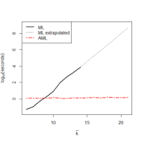
We now assess the performance of AML for a large value of . We choose and other parameter values that resulted from the empirical example conducted later (see Table 4 in the following subsection). Figure 5 displays the estimation results over 1,000 Monte Carlo replications from the DGP associated with (as in the empirical dataset in the following subsection), and where the parameter values are , , , and . For each sample, we calculate the constrained estimator and AML estimator using pseudo-samples. For each sub-figure, the left plot contains the constrained auxiliary estimates and the right plot contains the associated AML estimator. The true parameter values are reported with horizontal lines. While the restricted model is easy to estimate, it provides estimators that are significantly biased for all parameters except . AML corrects the resulting bias for all structural parameters and delivers estimators that are, on average, centred over the true values. Analyzing the other accuracy measures given in Table 3, we see that AML generally yields estimators with low bias and Monte Carlo coverage close to the nominal level.

| Auxiliary | Bias | 0.363348 | -0.061777 | 12.002244 | 0.000943 | - |
| MSE | 0.133257 | 0.003867 | 174.209123 | 0.000014 | - | |
| COV | 0.000000 | 0.000000 | 0.480000 | 0.939000 | - | |
| AML | Bias | -0.001502 | 0.012439 | 0.025719 | 0.000033 | -1.558178 |
| MSE | 0.000303 | 0.002176 | 0.022416 | 0.000009 | 11.391885 | |
| COV | 0.936000 | 0.955000 | 0.937000 | 0.945000 | 0.897000 |
Application: S&P500 Returns
We now estimate the Binomial MSM model (with ) on demeaned daily SP500 (simple) returns between January 3, 1928 and May 15, 202088 8 Downloaded from finance.yahoo.com on May 15, 2020.. The sample size is . The data are plotted in Figure 6. Using this data, Table 4 compares the AML estimators with those obtained from maximum likelihood for fixed values of ranging from up to . The estimated value of obtained by AML is far larger than the feasible value associated with ML. Moreover, except for , the remaining estimated parameters are also significantly different, with the estimated values of and being markedly different across the two approaches. The standard errors for ML are calculated using the asymptotic formula, while those for AML are calculated using a parametric bootstrap based and 1,000 simulated data sets from the assumed DGP.
In order to compare the goodness-of-fit of the eleven models enumerated in Table 4, for each model we provide one-day-ahead forecasts at each in-sample date using a particle filter of size . For a given model, at each date , the particle filter provides simulated values from the approximate distribution of :
At each date , we calculate the and value-at-risk forecasts defined by
where indicates the -th sample quantile, and report the failure rate of :
The closer is to , the better the forecasts. The left panel of Table 6 reports for and for each model specification along with asymptotic standard errors in parentheses. AML provides the only model specification for which both failure rates are not significantly different from their nominal levels. In addition, we also assess the accuracy of the expected shortfall forecasts:
To this end, we collect the empirical returns satisfying , under the model with , and for each value of in Table 4, we regress these returns on , calculated under the corresponding value of in Table 4. Regression intercepts, slopes, values and -values of the Wald test associated with the joint hypothesis are reported in the right panel of Table 6. The specification provides the best expected shortfall forecasts, as measured by the magnitude of the corresponding -values.

| Log-like. | ||||||
|---|---|---|---|---|---|---|
| ML | 1 | - | 75476.07 | |||
| 2 | 76409.45 | |||||
| 3 | 76779.51 | |||||
| 4 | 76874.11 | |||||
| 5 | 76940.79 | |||||
| 6 | 76978.39 | |||||
| 7 | 76994.82 | |||||
| 8 | 77001.80 | |||||
| 9 | 77006.94 | |||||
| 10 | 77009.94 | |||||
| AML | - |
| VaR failure rates | regressions | ||||||
|---|---|---|---|---|---|---|---|
| Intercept | Slope | Wald | |||||
| ML | 1 | 0.4771 | |||||
| 2 | 0.6015 | ||||||
| 3 | 0.6331 | 0.0013 | |||||
| 4 | 0.6420 | 0.1256 | |||||
| 5 | 0.6420 | 0.0151 | |||||
| 6 | 0.6149 | ||||||
| 7 | 0.6127 | 0.0115 | |||||
| 8 | 0.6215 | 0.0741 | |||||
| 9 | 0.6236 | 0.0725 | |||||
| 10 | 0.6271 | 0.1981 | |||||
| AML | 18 | 0.6412 | 0.2022 | ||||
5 Conclusion
In this paper, we provide an alternative to indirect inference (hereafter, I-I) estimation that simultaneously allows us to circumvent the intractability of maximum likelihood estimation (as with standard I-I), but which, in contrast to naive I-I, respects the goal of obtaining asymptotically efficient inference in the context of a fully parametric model. Although close in spirit to I-I, the approximate maximum likelihood (hereafter, AML) method developed in this paper does not belong to the realm of I-I for two reasons: First, the asymptotic distribution of the AML estimator only depends on the probability limit of the estimated auxiliary parameters and not on its asymptotic distribution. Second, while the AML estimator is obtained by matching two sample moments, one computed on observed data, and one computed on simulated data, both sample moments depend on the observed data through the value of the preliminary estimator of the auxiliary parameters. Interestingly, the sampling uncertainty carried by this preliminary estimator has no impact on the asymptotic distribution of the AML estimator because it is erased through the matching procedure.
The message of our paper is threefold. First, we demonstrate that the idea of matching proxies of the score for the structural model seems productive to reach near efficiency for inference on the structural parameters. We show theoretically that, at least for exponential models or transformation of them, the efficiency loss should be manageable since it is mainly due to the effect of a misspecification bias created by our simplification of the structural model.
Second, there are many non-linear time series models, which are popular in financial econometrics and dynamic/nonlinear microeconometrics, where a natural simplification of the structural model yields a convenient proxy for the score of the structural model. Since the misspecification bias created by this simplification is only due to imposing some possible false equality constraints, or to numerical approximations for certain elements of the gradient vector, one may reasonably hope that the resulting efficiency loss is minimal. While our general results (and theoretical examples) suggest that this finding is valid in many examples, including dynamic discrete choice and stochastic volatility models, we provide numerical evidence in three specific examples: generalized Tobit, Markov-switching multifractal models and stable distributions. The numerical results largely confirm our intuitions. Our method can alleviate the computational cost of maximum likelihood associated with complex models, at the cost of a limited loss in efficiency. Moreover, we confirm that even in finite-samples, the Wald confidence intervals associated to AML estimators display excellent coverage, since, thanks to matching the misspecification bias, the preliminary estimators have no impact on the central tendency of the AML estimator.
A third and even more general message is that the matching principle put forward by I-I estimation can be extended to situations where the two empirical moments to match, one based on observed data, one based on simulated data may both depend on the observed data through a convenient summary of them. While we have used this idea to aim for (nearly) efficient inference, Gospodinov, et al., (2017) employ a similar approach to hedge against misspecification bias due to the use of a misspecified simulator. Even though they have not derived the asymptotic distribution theory in their case, the two methods are essentially similar and could be nested within a general asymptotic theory where both the moments to match and the simulator depend on observed data.
References
- [1] Amemiya, Takeshi. Advanced econometrics. Harvard university press, 1985.
- [2] Bansal, Ravi, and Amir Yaron. “Risks for the long run: A potential resolution of asset pricing puzzles.” The Journal of Finance 59, no. 4 (2004): 1481-1509.
- [3] Behrens, S. and Melissinos, A.C., Univ. of Rochester Preprint UR-776 (1981).
- [4] Calvet, Laurent E., and Veronika Czellar. “Through the looking glass: Indirect inference via simple equilibria.” Journal of Econometrics 185, no. 2 (2015): 343-358.
- [5] Calvet, Laurent, and Adlai Fisher. “Forecasting multifractal volatility.” Journal of Econometrics 105, no. 1 (2001): 27-58.
- [6] Calvet, Laurent E., and Adlai J. Fisher. “How to forecast long-run volatility: Regime switching and the estimation of multifractal processes.” Journal of Financial Econometrics 2, no. 1 (2004): 49-83.
- [7] Calvet, Laurent E., and Adlai Fisher. Multifractal volatility: theory, forecasting, and pricing. Academic Press (2008).
- [8] Calzolari, Giorgio, Gabriele Fiorentini, and Enrique Sentana. “Constrained indirect estimation.” The Review of Economic Studies 71, no. 4 (2004): 945-973.
- [9] Chambers, John M., Colin L. Mallows, and B. W. Stuck. “A method for simulating stable random variables.” Journal of the american statistical association 71, no. 354 (1976): 340-344.
- [10] Chen, Fei, Francis X. Diebold, and Frank Schorfheide. “A Markov-switching multifractal inter-trade duration model, with application to US equities.” Journal of Econometrics 177, no. 2 (2013): 320-342.
- [11] Dridi, Ramdan, Alain Guay, and Eric Renault.“Indirect inference and calibration of dynamic stochastic general equilibrium models.” Journal of Econometrics 136, no. 2 (2007): 397-430.
- [12] Dudley, Leonard, and Claude Montmarquette. “A model of the supply of bilateral foreign aid.” The American Economic Review 66, no. 1 (1976): 132-142.
- [13] Franses, Philip Hans, Marco Van Der Leij, and Richard Paap. “A simple test for GARCH against a stochastic volatility model.” Journal of Financial Econometrics 6, no. 3 (2008): 291-306.
- [14] Frazier, David T., and Eric Renault. “Indirect inference with(out) constraints.” Quantitative Economics, 11 (2020): 113-159.
- [15] Frazier, David T., Tatsushi Oka, and Dan Zhu. “Indirect inference with a non-smooth criterion function.” Journal of Econometrics 212, no. 2 (2019): 623-645.
- [16] Gallant, A. Ronald. and George Tauchen. “Which moments to match.” Econometric Theory 12, (1996): 657-681.
- [17] Gospodinov, Nikolay, Ivana Komunjer, and Serena Ng. “Simulated minimum distance estimation of dynamic models with errors-in-variables.” Journal of econometrics 200, no. 2 (2017): 181-193.
- [18] Gourieroux, Christian, Alain Monfort, and Alain Trognon. “Pseudo maximum likelihood methods: Theory.” Econometrica: Journal of the Econometric Society (1984): 681-700.
- [19] Gourieroux, Christian, Alain Monfort, and Alain Trognon. “A general approach to serial correlation.” Econometric Theory 1, no. 3 (1985): 315-340.
- [20] Gourieroux, Christian and Alain Monfort. Simulation-based Econometric Methods, OUP, (1996).
- [21] Gourieroux, Christian, Alain Monfort and Eric Renault. “Indirect inference.” Journal of Applied Econometrics 85, (1993): S85–S118.
- [22] Gourieroux, Christian, Alain Monfort, Eric Renault, and Alain Trognon. “Generalised residuals.” Journal of Econometrics 34, no. 1 (1987): 5-32.
- [23] Hansen, Lars Peter. “Large sample properties of generalized method of moments estimators.” Econometrica: Journal of the Econometric Society (1982): 1029-1054.
- [24] Koutrouvelis, Ioannis A. ”An iterative procedure for the estimation of the parameters of stable laws: An iterative procedure for the estimation.” Communications in Statistics-Simulation and Computation 10, no. 1 (1981): 17-28.
- [25] Louis, Thomas A. “Finding the observed information matrix when using the EM algorithm.” Journal of the Royal Statistical Society: Series B (Methodological) 44, no. 2 (1982): 226-233.
- [26] McCulloch, J. Huston. “Simple consistent estimators of stable distribution parameters.” Communications in Statistics-Simulation and Computation 15, no. 4 (1986): 1109-1136.
- [27] Meddahi, Nour, and Eric Renault. “Temporal aggregation of volatility models.” Journal of Econometrics 119, no. 2 (2004): 355-379.
- [28] Pinkse, Joris, and Margaret E. Slade. “Contracting in space: An application of spatial statistics to discrete-choice models.” Journal of Econometrics 85, no. 1 (1998): 125-154.
- [29] Poirier, Dale J., and Paul A. Ruud. “Probit with dependent observations.” The Review of Economic Studies 55, no. 4 (1988): 593-614.
- [30] Robinson, Peter M. “On the asymptotic properties of estimators of models containing limited dependent variables.” Econometrica, (1982): 27-41.
- [31] Smith, Anthony A. “Estimating nonlinear time series models using simulated vector autoregressions.” Journal of Applied Econometrics 8, no. S1 (1993): S63-S84.
- [32] van der Vaart, Aad W. Asymptotic statistics. Vol. 3. Cambridge university press, 1998.
Appendix A Proofs of Main Results
A.1 Proof of Proposition 1
With standard abuse of notation, a Taylor expansion gives:
where and are all in the interval Hence:
with, thanks to assumptions A1 and A2, and the fact that
implies that our AML estimator is such that:
Under assumption A3, an additional Taylor expansion gives
where are all in the interval Hence:
We know from Gourieroux, Monfort and Renault (1993) (see their proposition 3 and its proof) that:
which completes the proof of Proposition 1.
A.2 Proof of Proposition 5
By virtue of Proposition 4, we only need to prove that the asymptotic variance of the UAML estimator coincides with the Cramer-Rao efficiency bound when . When , this estimator, denoted , can be seen as the solution in of the system of equations:
If we define
we have, by definition,
Recall the definition of ,
| (27) | |||||
and note that, by virtue of (27),
converges in distribution to a random variable, where is the Fisher information matrix.
Moreover,
and we have
where denotes some dominating measure. Thus,
Therefore,
is the Fisher information matrix . Consequently,
Appendix B GARCH-like Stochastic Volatility Models: Pseudo-Score
To this end, we first compute the latent score, and then use this to interpret the score in terms of generalized residuals, it is worth computing the latent score. We first decompose the latent log-likelihood as follows:
Computations very similar to the case of Gaussian QMLE of ARCH models give:
while
where is the derivative of the probability density function . Note that for sake of non-negativity of variance, we expect the probability distribution of to have a lower bounded support, like for instance a demeaned log-normal distribution. However, it is a reasonable hypothesis to see as a Gaussian variable if we consider that the correction term is small enough such that a Gaussian approximation is accurate enough. We would then get a proxy of the latent score by:
The message from (17) is that we will go from latent score vector to observable one by replacing all functions of latent volatility by its optimal filter. Let us define these filters:
| (28) | |||||
Then, we have
We recall that we denote these pseudo-score components with notation to stress that they are only approximations. They have been computed with filtering formulas (28) that are only approximations since doing as if The filtered values (28) allow us to compute ”generalized residuals” similar to the one computed in the dynamic Probit example. However, by contrast with this example, we do not have in general closed form formulas for these filters. Any filtering strategy may be worth applying in this context. At least, a very simple one is to use the approximation as a convenient filter, meaning that we replace in all filtering formulas , the latent quantity by the observed one (erasing then the conditional expectation operator) that comes from fitting an model to our data set .
We now address the computation of the partial derivative of the observed log-likelihood with respect to the parameter .
Using the definition of the latent likelihood, see Section 2.2.2, we can write:
where
Then,
With an innovation process that is a standard Gaussian, this leads (by computing the derivative of the product as a sum of products with one term differentiated in each) to:
| (29) | |||||
where is the sample autocovariance of order of the latent process
Appendix C Details for Examples in Section 3
In this section, we give the details required to obtain Result 2 in Section 3. In addition, we also extend this example to consider latent exponential models.
C.1 Example: Exponential Models
For the sake of exposition, we assume that conditionally on , the variables are independent and the conditional distribution of only depends on the exogenous variable with the same index. This distribution has a density that is assumed to be exponential:
where and are given numerical functions and and are -dimensional random vectors. Note that the extension to dynamic models in which conditioning values would also include some lagged values of the process would be easy to devise. From:
we deduce, since the conditional score vector has by definition a zero conditional expectation, that:
Following Theorem 1 in Gourieroux et al. (1987),
Therefore, the maximum likelihood estimator is defined as solution of:
| (31) |
We actually generalize the remark of van der Vaart (1998), Section 4.2., noting that ”the maximum likelihood estimators are moment estimators” based on the (conditional) expectation of the sufficient statistic . The first-order conditions (31) show that maximum likelihood is the GMM estimator with optimal instruments for the conditional moment restrictions:
Note that we implicitly maintain the assumptions for standard asymptotic theory of efficient GMM (Hansen, 1982): for all , the conditional variance of the moment conditions is non-singular and the Jacobian matrix is full row rank.
The identification condition for consistency of maximum likelihood is then that:
In terms of GMM, it means that optimal instruments are assumed to identify the true unknown value of the parameter vector , by contrast with cases put forward by Dominguez and Lobato (2004). By the Law of Iterated Expectations, this can be rewritten:
or equivalently (by symmetry):
| (32) |
By extension of (31), we have:
| (33) |
so that:
Hence:
By the Law of Iterated Expectations:
so that the identification Assumption B1 amounts to:
| (34) |
When , we are back to the well-specified example and (34) is obviously identical to the identification condition (32) for consistency of maximum likelihood.
Moreover, the identification assumption (34) for consistency of the UAML estimator is clearly likely implied by the standard condition (32) for consistency of maximum likelihood, at least in two particular cases:
1st case: The model is a linear regression model w.r.t. some known multivariate function of :
In this case, the identification condition (34) is akin to:
Obviously, when the matrix:
is positive definite for , it is positive definite for any possible value of .
2nd case: The model is not conditional. In this case, a necessary condition for identification condition is:
| (35) |
This is basically the case considered by van der Vaart (1998) when noting that ”the maximum likelihood estimators are moment estimators” based on the expectation of the sufficient statistic . This identification condition should be maintained when picking linear independent equations out of possibly overidentified equations (35). More precisely, the identification condition for UAML, written as:
should generically be implied by (35), since, irrespective of the value of , the matrix is full row rank.
More generally, one may expect that the identification condition (34), when fulfilled for , should be more often than not fulfilled for any value of .
C.2 Example: Latent Exponential Model
We now extend the exponential model example to incorporate a sequence of latent variables , such that, conditionally on , the variables are independent, for all , and the conditional distribution of only depends on the exogenous variable with the same index. This distribution has a density , with respect to the dominating measure , that is assumed to be exponential:
Let be a known vector function that defines the observed endogenous variable as:
Then, conditionally on , the variables are independent and the conditional distribution of only depends on the exogenous variables with the same index. This conditional distribution has a density , with respect to the measure , which is the transformation of the original measure by , and where we recall that was the dominating measure used to define the latent density . The observable log-likelihood can then be stated as
In general, the observable density is not of an exponential form, see Gourieroux et al. (1987) for the particular case where and for examples of Probit, bivariate Probit, Tobit, generalized Tobit, disequilibrium and Gompit models. As already mentioned in Section 2.3, Gourieroux et al. (1987), extending a result of Louis (1982), give a method to compute the observable score as a conditional expectation of the latent score
Then, by applying (31) we get
| (36) |
As exemplified by Gourieroux et al. (1987) for many limited dependent variable models, we can define and compute a generalized error as:
Then, the maximum likelihood estimator is defined as solution of
| (37) |
Hence, the identification condition for consistency of maximum likelihood can be written:
| (38) |
We also note that MLE is not any more a moment estimator with optimal instruments (confirming that the model is not exponential any more) since:
More generally, by extension of (37) we have:
Hence,
so that
When , we are back to the well-specified example and we note that by definition:
so that the identification condition
can be written
| (39) |
By commuting the roles of and , this is clearly tantamount to the identification condition (38) for maximum likelihood. In the general case, the identification condition B1( for UAML can be written:
Note that by the Law of Iterated Expectations, this can be written:
where
By comparison with (39), we see that while both generalized errors and will in general have a non-zero conditional expectation given (when ), identification means that when , their difference cannot be orthogonal to the specific functions of that define the rows of the selection matrix:
This condition is similar to the condition (34) of identification for UAML in the exponential model example, except that, due to the transformation , the conditional expectation given along simulated paths still depend on . In the particular case of a latent model defined by a univariate linear and homoskedastic regression equation:
the identification condition in Assumption B1 for UAML becomes:
For instance, in the case of a Probit model ():
which we can compare to the standard identification condition for a Probit model
These conditions appear to be quite reasonable.
Appendix D Example 5: (Stable Distribution)
Consider i.i.d. observations generated from a stable distribution with stability parameter , skewness parameter , scale parameter and location parameter . The structural parameter vector is given by
We consider this model under the false equality constraint:
corresponding to a Cauchy distribution with location and scale , which gives the log-likelihood:
We can define the pseudo-score vector as:
Note that, the finite difference is a convenient approximation of the partial derivative since the log-likelihood function is computed as the likelihood for i.i.d. draws in a Normal distribution with mean and variance . Second, the finite difference is a convenient approximation of the partial derivative since the log-likelihood function could be computed as the likelihood for i.i.d. draws in a Landau distribution with location parameter and scale parameter
To speed up the computation, we use the following approximation to given by Behrens and Melissinos (1981).99 9 Similar results were obtained whether or not the approximation was employed. Given the similarity of the results, and the drastic speed difference, the approximation approach is more reasonable to apply in practice.
D.1 Monte Carlo
We now compare the behavior of AML using the above pseudo-score, and simulations, against two alternative approaches: one based on sample quantiles, due to McCullough (1986), and one based on an auxiliary regression model, due to Koutrouvelis (1981). To this end, we generate 1,000 synthetic datasets from the alpha stable models, each with observations, and under .
We display the resulting estimators across the replications in Figure 7.1010 10 We remark that while ML estimation is feasible in the -stable model for small numbers of observations, given the sample size considered herein, obtaining the MLE proved to be computationally infeasible. Analyzing the results, we see that the three procedures perform similarly for , but display different behavior for , although all estimators seem quite reliable, and are well-centred over the true values.
Table 7 records the Monte Carlo bias (Bias), root mean squared error (RMSE), and Monte Carlo coverage (COV), based on individual 95% Wald interval, across the replications. The results demonstrate that the methods all yield accurate estimators of the corresponding true values. However, we note that the simpler methods do outperform AML in terms of bias and RMSE, but display worse coverage than AML in almost all cases.
| AML | Aux | Kout | McC | AML | Aux | Kout | McC | |||
|---|---|---|---|---|---|---|---|---|---|---|
| Mean | 1.8190 | 1.0000 | 1.7994 | 1.8031 | Mean | -0.0948 | 0.0000 | -0.0966 | -0.1039 | |
| Bias | 19.0315 | -800.0000 | -0.6072 | 3.1120 | Bias | 5.1846 | 100.0000 | 3.4381 | -3.8520 | |
| RMSE | 9.6607 | 80.0000 | 1.4561 | 2.9785 | RMSE | 13.6959 | 10.0000 | 6.5433 | 7.9542 | |
| COV | 0.9600 | 0.0000 | 0.9410 | 0.9540 | COV | 0.9650 | 0.0000 | 0.9540 | 0.9440 | |
| AML | Aux | Kout | McC | AML | Aux | Kout | McC | |||
| Mean | 0.1002 | 0.0881 | 0.1000 | 0.1000 | Mean | 0.0007 | 0.0025 | 0.0032 | 0.0031 | |
| Bias | 0.1636 | -11.8524 | 0.0016 | -0.0074 | Bias | 0.6945 | 2.4720 | 3.2351 | 3.1469 | |
| RMSE | 0.1488 | 1.1884 | 0.0978 | 0.1251 | RMSE | 0.6313 | 0.2986 | 0.3737 | 0.3781 | |
| COV | 0.9480 | 0.0000 | 0.9480 | 0.9510 | COV | 0.9810 | 0.6650 | 0.6030 | 0.6640 |