Dark Matter with -Body Numerical Simulations
Abstract
Abstract
The development of numerical -body simulations have allowed to study formation process and evolution of galaxies at different scales. This paper presents the fundamental concepts of -body systems applied to the cosmological evolution of the -Cold Dark Matter (CDM) model. In order to perform structure formation in the Universe, we provide an introduction to the basic equations and their implementation on the GADGET-2 software. We also present a simple guide to modify this code. First, we briefly describe the dark matter in the Universe as well as the theoretical and experimental basis of the CDM model. Then, we focus on the simulation codes and provide the equations that govern most of the -body simulations to model the dark matter. We describe the Smoothed Particle Hydrodynamics method used for simulating the gas, star dynamics and structure formation in these simulations. Then, cautiously, we guide the reader to the installation of GADGET-2 on a Linux-based computer, as well as to carry out a couple of examples to operate the code. Finally, by using a computational cluster, we show several results of a large structure simulation, analyse the outputs to display the matter power spectrum, and compare the outcome with theoretical predictions.
Keywords—Numerical Simulations, -body systems, cosmology, CDM
1 Introduction
Over recent decades cosmology has played an important role in the development of science and technology. Its main goal seeks to explain the origin and evolution of the Universe as a whole, and hence, the fundamental physics behind those process to therefore gain a deeper understanding of the laws of physics 2003itc..book…..R. It is well known that the observable matter, galaxies, stars, gas clouds, planets and so on only contribute to about of the total content of the Universe, whereas corresponds to an unknown dark matter – with the property to be gravitationally attractive – responsible to be the main component of structure formation, and the remaining corresponds to the dark energy – the main candidate to explain the current accelerated expansion of the Universe. These results conform the most well established model for the evolution of the Universe, the -Cold Dark Matter model (CDM).
Nonetheless, CDM has been tested throughout the years using diverse experiments, just like the Planck mission and going back through other similar surveys, for example: the WMAP mission results in 2007 2007ApJS..170..377S, as well as the measured fluctuations in the CMB temperature by the COBE satellite in 1994 1994ApJ…420..439M. All of them, amongst many others, have contributed to reinforce the foundation of the CDM model. One of the essential tests come from the -body simulations, which are able to constrain several cosmological parameters. The key procedure of the -body simulations is to evolve bound systems by considering dark matter interacts only gravitationally with ordinary matter. This paper focuses on the basis for these kind of simulations in order to provide an understanding of the cosmological evolution, through some commonly used codes.
The paper is structured as follows: First we provide a brief review about dark matter and its importance on the development of the CDM model. Then, we present some numerical codes and their use on astrophysical systems, followed by the -body simulations and their basic equations. We include a section dedicated to Smoothed Particle Hydrodynamics (SPH) and how to simulate gas dynamics. Later, we introduce the GADGET-2 software, a -body-SPH hybrid free source code used in this work, and the basic installation procedure. Finally, by running the code, we present some results given different simulations, in particular from the evolution of two isolated galaxies colliding and merging into a larger galaxy, and also from the cosmological evolution of a periodic box described by a CDM Universe. For the second example, we compute the matter power spectrum -an important quantity used to constrain physical quantities for a given cosmological model-.
Dark Matter
The beginning of dark matter history may be traced back to 1937 when the astrophysicist Fritz Zwicky examined the internal dynamics of the Coma Berenice galaxy cluster 1937ApJ….86..217Z. In that work, Zwicky provided evidence that the luminous mass in the cluster was much smaller than the total mass needed to hold these galaxies together by gravitational forces. Therefore, he concluded that there should be another type of matter that would allow galaxies to be gravitationally bounded. These observations were the first hints of a missing matter in galaxy clusters, – the “dark matter” made its first appearance in the scientific community ever since –.
Despite numerous contributions from the scientific community, the issue of the dark matter was not seriously considered until the early years of the 1970 decade, when the astronomer Vera Cooper Rubin indicated that the gravitational stability of galaxies is due to an amount of mass greater than the observed 1970ApJ…159..379R. In her work, she calculated the rotational curves of different spiral galaxies by measuring the radial velocity of the stars located at a distance from the galaxy center, as seen in the following equation
| (1) |
where is the Newton gravitational constant and is the mass contained within the radius . According to Newton’s laws, this movement is expected to be Keplerian, that is, the velocity of the stars would decline as the distance increases. The big surprise was that this curve does not follow the expected behaviour, as observations showed that the speed of the stars remained almost constant, and even in some cases it increased. If Newton’s theory is correct, then a new kind of mysterious matter is needed whose mass distribution must increase with the radius. This strange behaviour is not observed on the Baryonic matter, which is distributed in a compact manner and its mass is not sufficient to maintain the flat rotation curve. The introduction of a new component caused a great impact on physics and astronomy, since it led to create alternative models that include dark matter in the galaxies, and therefore, also in the Universe.
Another evidence is the Cosmic Microwave Background (CMB) 1965ApJ…142..419P as being the earliest photograph of the Universe. The patterns seen on the CMB were set up by two competing forces acting upon matter: the gravity, causing the matter to fall inwards, and the radiation pressure, preventing the gravitational collapse. This competition caused the photons and matter to oscillate in and out in dense regions forming patterns, that would be dramatically modified by the amount and type of dark matter present at that epoch. That is, the existence of dark matter leaves a characteristic imprint on CMB observations, as it clumps into dense regions and contributes to the gravitational collapse of matter, but it is unaffected by the pressure from photons. The CMB power spectrum shows the strength of these oscillations at different scales, and for instance, the Wilkinson Microwave Anisotropy Probe (WMAP) 2007ApJS..170..377S was able to measure with enough accuracy the CMB spectrum and consequently favoured the existence of dark matter.
Dark matter is also highly favoured when the Large Scale Structure formation is studied. The oscillations imprinted on the CMB evolved into more advanced structures, given the amount of time available for objects to gravitationally collapse, eventually forming what is called the Baryon Acoustic Oscillations (BAO). At the time of CMB, dark matter did not undergo to the same oscillations with matter and light, but it was free to collapse on its own, this created dense regions that helped structure formation. Ths mechaninsm allowed the distribution of galaxies and clusters to be what it is observed today 2017AJ….154…28B.
Lambda Cold Dark Matter (CDM)
As mentioned above, one of the first predictions of the existence of dark matter was made by Zwicky. This result came from his observations on the Coma cluster in order to be able to explain its strange dynamics that would not match with a Newtonian behaviour. Although these observations were truly remarkable by that time, it wasn’t until the 1980 decade that both astronomers and physicists concluded that one way to explain the movement of the galaxies, according to Newtonian dynamics, was to include the “missing” matter predicted by Zwicky in the equations of motion.
The introduction of this missing matter (as well as the cosmological constant ) conforms the Lambda Cold Dark Matter model. It is a parametrization to describe the cosmological Big Bang model and nowadays is referred as the “standard cosmological model”, which is based on the following theoretical and experimental facts:
- •
A theoretical framework based on General Relativity, which provides a field theory for gravitation on cosmological scales.
- •
The cosmological principle: the Universe is spatially isotropic and homogeneous on large scales 2003itc..book…..R.
- •
The perfect fluid model: the galaxies and the basic components of the Universe are included within the theory via the continuity equation schutz:2009.
- •
The Hubble’s law establishes the expansion of the Universe in which the galaxies recession velocity is proportional to their distance 1929PNAS…15..168H.
- •
The Cosmic Microwave Background radiation (CMB). The measurements of the CMB radiation support the cosmological principle on large scales 1965ApJ…142..419P; 2007ApJS..170..377S; 2013IJMPD..2230029M.
- •
The determination of the relative abundance of primordial elements such as 1H, 2D, 3He, 4He and 7Li, made up on nuclear reactions during the Big Bang Nucleosynthesis (BBN) era 1993ppc..book…..P.
- •
The large scale structure analysis of the Universe using data from the Sloan Digital Sky Survey (SDSS) 2017AJ….154…28B, that aids the parameter determination of the standard cosmological model.
Moreover, the CDM model adds some other special features that allow to explain the evolution of the structure in the Universe:
- •
The evolution of matter density perturbations, initially coming from quantum density fluctuations, is required to explain the large scale structure in the Universe 10.1143/PTP.76.1036.
- •
The Cosmic Inflation, originally introduced by Alan Guth, postulates an accelerated expansion at very early times that allows to explain the homogeneity and flatness in the Universe, as it is observed today 1981PhRvD..23..347G.
- •
The cosmological constant , introduced by Einstein on his equations of general relativity to force a static Universe. Nevertheless, it is known today that the Universe is in an accelerated expansion and this constant is referred to a form of vacuum energy or some kind of dark energy 2003RvMP…75..559P.
- •
Cold Dark Matter (CDM). A sort of matter that has an exclusive gravitational attraction, does not interact with any kind of radiation (it is dark) and its velocity is not relativistic (it is cold).
Some known issues with CDM
Although this model has been successfully proved by several observations and theoretical predictions,
it has certain inconsistencies or unexplained features mainly on small scales.
Two of them are
CUSP-CORE problem. It refers to a discrepancy between the inferred dark matter density profiles of low-mass galaxies and the density profiles predicted by cosmological -body simulations. Nearly all simulations with cold dark matter form halos which have “cuspy” distributions, with density increasing steeply at small radii, whereas the rotation curves of most observed dwarf galaxies suggest that they have flat central dark matter density profiles 1996ApJ…462..563N; 1997ApJ…490..493N; Moore:1994yx.
Missing satellite problem. It arises from a mismatch between observed dwarf galaxy numbers and numerical cosmological simulations that predict the evolution of the distribution of matter in the Universe. In simulations, dark matter clusters hierarchically, increasing the numbers of halo “blobs” as halo components become smaller-and-smaller. However, there seem not to be enough observed normal-sized galaxies to match the simulated size distribution; the number of dwarf galaxies is orders of magnitude lower than expected from simulation1999MNRAS.310.1147M; 2005Natur.435..629S.
With these deficiencies in mind, several alternative models have been suggested. Of a particular interest is to consider that the Dark Matter is made up of bosonic excitations of an ultra-light scalar field minimally coupled to gravity, see Matos:2008ag; Magana:2012ph; Hui:2016ltb and references therein. We defer the numerical analysis with scalar fields for a future work.
2 Numerical Codes for astrophysical systems
To understand the large scale formation and structure of the Universe, the gravitational instability on cosmological scales and galaxy evolution, numerical -body simulations are one of the most used approaches. Over recent years, the computational resources have allowed to create high resolution simulations that recreate the evolution of the Universe since the CMB epoch (). Cosmological evolution is simulated with linear gravitational clustering on large scales ( Mpc) and non-linear theory on small scales (between 10 kpc and 1 Mpc). On small scales, specific initial conditions are created to evolve the dark matter particles, with the consideration that the dynamics can be enhanced by introducing effects of gas dynamics, chemical process, radiative transfer and other astrophysical phenomena.
There is a large variety of numerical codes that use the -body theory and several applications including gas dynamics modelled by Smoothed Particle Hydrodynamics (SPH). These codes have been used in numerous times, and they have proved being a realistic approach according to observations. We list some of the methods used below:
- 1.
Direct methods: these do not introduce approximations but they fully solve the equations of motions and thus deliver the highest accuracy at the price of the longest computation time, of order per timestep. Integration is performed using adaptive (individual) timesteps and commonly a fourth order Hermite integrator Mikkola1993.
- 2.
Tree codes: The tree code method (Barnes & Hut 1986) provides a general integrator for collisionless systems. They take into account that particles nearby each other are important and the contributions from distant particles does not need to be computed with high accuracy, while potentials from distant groups of particles are approximated by multipole expansions about the group centres. The resulting computation time scales as but the approximations introduce small force errors. The long-range force errors are controlled by a single parameter (the opening angle) that determines how small and distant a group of particles must be to use the approximation. Typical implementations of the tree code is to expand the potentials to quadrupole order and construct a tree hierarchy of particles using a recursive binary splitting algorithm. The tree does not need to be recomputed from scratch at every timestep, saving significant CPU time 1986Natur.324..446B.
- 3.
Particle-mesh codes: This method is used as another approximation to speed up direct force calculation for collisionless systems. In this case the gravitational potential of the particular system is constructed over a grid starting from the density field and solving the associated Poisson equation, by using Fast Fourier Transform. Particles do not interact directly amongst each other but only through a mean field. This method essentially softens the gravitational interactions at small scales. The density field is constructed using a kernel to split the mass of the particles to the grid cells around the particle position. In a short range, accuracy of the force is a poor approximation of Newton’s law up to several grid spacing distance klypin1997particlemesh.
- 4.
Adaptive Mesh Refinement method: Particle-mesh codes can be enhanced by using an adaptive method rather than a static grid to solve the Poisson Equation. In the Adaptive Mesh Refinement (AMR) method the grid elements are concentrated where a higher resolution is needed, for example around the highest density regions. To obtain an adaptive resolution the method first uses a low-resolution solution of the Poisson equation, and then, progressively refining regions where a higher resolution is required 2004astro.ph..3044O.
2.1 Basic -body equations of motion
It is well known that Einstein field equations describe the space-time behaviour in the presence of matter, that is
| (2) |
where is the Ricci tensor, is the Ricci scalar, is the metric tensor, is the cosmological constant, and is the energy-momentum tensor. For a homogeneous and isotropic space-time, the energy-momentum tensor needs to be homogeneous and isotropic as well. This tensor is also known as a perfect fluid tensor and it has the following form
| (3) |
inserting equation (3) into equation (2) and setting , for a FRW metric with scale factor , we obtain the Friedmann equations:
In the CDM model, dark matter is assumed to be a non-baryonic matter component and its interaction is only gravitational, hence non-collisional. The -body problem for these systems is described by the non-collisional Boltzmann equation in comoving coordinates coupled with the Poisson equation. A system of particles interacting gravitationally defines a 6 dimensional phase space given by the positions and velocity vectors associated to each particle at each time . The solution of the -body problem defines a trajectory in this phase space. On the other hand, if the number of particles is large enough, that is, if the two body relaxation time is long compared to the time-frame of interest, then a statistical description of the problem is possible. This allows to map the computation from a 6 dimension to a 6+1 dimension phase space. The idea is to construct a mean field description of the dynamical system in terms of a single particle distribution function. The Boltzmann equation describes the behaviour and evolution of a fluid in the phase-space under external forces and has the following form
| (4) |
where is the distribution function of the density of the fluid, is the velocity, is the position, is the force and is the mass of an individual particle of the system, that can describe eventually all the fluid. If the force is derived from a gravitational potential , it follows that
| (5) |
Substituting equation (5) in (4), it can be written as
| (6) |
This potential must satisfy Poisson’s equation
| (7) |
where represents all space described by the total mass enclosed in a cube of volume centred in and velocity located in a cube of volume centred in . When integrating all over the space, the result is that the mass density may depend of time (), therefore, Poisson’s equation described in equation (7) can be reduced to a more familiar way.
Given its high dimensionality (6+1), the collisionless Boltzmann equation is usually solved by sampling the initial distribution function , and then, evolving the resulting -body system, for instance with a numerical method that suppresses two body interactions at small scales. The interaction is softened not only for computational convenience to limit the maximum relative velocity during close encounters but especially to prevent artificial formation of binaries.
In its discrete form, the Boltzmann equation describes the evolution of a set of point masses that auto interact gravitationally. In an -body system, if is the coordinate and is the mass of each particle, then Newton’s equations of motion are
| (8) |
using comoving coordinates related with the physical coordinates via the scale factor , it follows that The evolution of the scale factor defines the Hubble factor , through the Friedmann equation, as
| (9) |
km s-1 Mpc-1 is the Hubble’s constant value at the present time, are the radiation, matter and dark energy densities, respectively, and their sum must be one for a flat Universe.
In an expanding space modelled by a periodic box of size , Newton equations of motion can be deduced, in comoving coordinates, as
| (10) |
| (11) |
where the sum over is affecting the particles and is the peculiar gravitational potential
| (12) |
related to the Newtonian potential of a density fluctuation around a constant background density. The sum over the particles is also extended over their corresponding periodic images, with being a triple integral vector. The factor is there to make sure that the mean density in Poisson’s equation (12) is different from zero, otherwise there would be no solution for an expanding space that tends to infinity. For a more detailed review, refer to the following reference springel2014high.
2.2 Smoothed Particle Hydrodynamics (SPH)
Smoothed Particle Hydrodynamics is needed to simulate astrophysical phenomena that involves
massive moving fluids in a 3-dimensional space. This method uses analytical differentiation
with interpolation to compute the space derivatives, unlike the -body approach, which divides
the space into cells to compute the force between particles. The SPH considers a set of
discrete particles which represent the state of the fluid with continuous quantities associated
to its motion, making the assumption that at any time, the position of the fluid elements are
randomly distributed but the density is conserved. Obtaining the density is equivalent to obtaining
the distribution probability of a fluid sample. An extended review of this topic can be found here
chacon_2019.
The existing methods are:
- •
Kernel softening. This method estimates the probability density function that describes the fluid parzen1962.
- •
The spline delta technique. A differentiable curve defined by polynomials that allows the data analysis and aids the continuous modelling of the fluid 1977MNRAS.181..375G; 1997JCoPh.136..298M.
2.3 Equations of motion
The three fundamental equations are the energy density conservation equation, the momentum conservation equation and the Poisson equation. These can be in their integral formulation or in their differential form. The set of equations is called Navier-Stokes, and for fluids without viscosity they represent the Euler equations. For cosmological simulations, the SPH approximation uses the perfect fluid model which is governed by the Euler equations of fluid dynamics, i.e. the continuity equation
| (13) |
and the momentum conservation equation
| (14) |
along with the Poisson equation
| (15) |
where are the density, velocity and pressure of the fluid at any time . This set of equations gives a global view of the fluid. In Lagrange’s representation, a point in the vector field is chosen at time , and then, the temporal evolution is analysed, which allows to study the particle dynamics that make up the fluid individually. By expressing the total derivative as
| (16) |
then, equation (13) takes the following form
| (17) |
and equation (14) can be written as
| (18) |
In order to describe a continuous fluid in a discrete approximation, SPH 1992ARA&A..30..543M starts by defining the integral interpolation of any function as
| (19) |
where the integration goes over all space and is an interpolation kernel that must satisfy
| (20) |
| (21) |
The limit corresponds to the interpolation of the integral and is a length parameter in a 3-dimensional space. Numerical computations lead to a sum approximation
| (22) |
where the index denotes each particle, and the sum is made over all the particles. Particle has mass , position , density , and velocity . Any other quantity inside is denoted by . The keypoint of this method is that it can build up a differentiable interpolator of any given function from its particular values (interpolation points) using an interpolation kernel that is also differentiable. There is no need of using finite differences or separating the space into cells just as -body does. If it requires to compute , the calculation is simply
| (23) |
The original calculations by Gingold & Monaghan (1977) 1977MNRAS.181..375G uses an unidimensional gaussian kernel
| (24) |
Nevertheless, to interpolate all over the nearest neighbours, a spline cubic function is usually defined as in the following reference (Springel et al. 2005 2005MNRAS.364.1105S)
| (25) |
This is the usual example that mimics a delta function in the limit . The choice of this kernel is such that the interaction recovers its Newtonian, original form at separations greater than the softening length (See 2.4.1). For a physical interpretation of the SPH equations it is better to assume a gaussian kernel, for example, the density at any point in space is approximated by
| (26) |
Using this interpretation, the fluid density is now expressed in a discrete form by using the interpolation functions. By doing so, the continuity (13), momentum conservation (14) and Poisson (15) equations pass from their continuous form to their discrete form, as described in reference 1985A&A…149..135M.
2.4 GADGET
GAlaxies with Dark matter and Gas intEracT (GADGET), is a free source code which uses the -body approach with SPH interpolation for cosmological simulations with its first version released in 2001 2005MNRAS.364.1105S. It is written in C language, and uses two main computational resources: Paralellization and the Tree–Particle Mesh Algorithm (TreePM). If a traditional method were used for computation purposes, it would require force calculations for the particles, and the order of the computation time goes as . The TreePM method reduces the time to an order of by collecting all the particles within a cube of a given minimum size, together with paralellization to allow the system of millions of particles be computed in a more efficient way without losing much resolution.
2.4.1 Gravitational softening
Because the large number of particles and information managed by the -body simulations, if two particles are really close in space, that would lead to a divergence in the force acting upon a pair of particles. In order to avoid this divergence and exceeding accelerations, if two particles are very close to each other, a gravitational softening is introduced which must be acting on the whole space of the simulation. This gravitational softening is there to prevent that particles within the simulated box come very close to each other, in other words, the gravitational softening acts as a constriction for the simulated particles, also allowing the particles to remain in the non-collisional regime needed to solve the Boltzmann equations. This is achieved by introducing a parameter into equation (8), as follows
| (27) |
where and is the softening length (Bodenheimer et al., 2007 2007nmai.conf…..B). The physical interpretation of is the distance between the two centers of two “binded” particles. There is no criteria for the choice of the value of , but for non-collisional systems, numerical results suggest using the mean separation between particles as a reference, although, it really depends on the size of the system that is being computed.
2.4.2 Tree–Particle Mesh algorithm and Paralellization
The tree particle method (Barnes & Hut 1986) 1986Natur.324..446B provides a fast, general integrator for collisionless systems, when close encounters are not important and where the force contributions from very distant particles do not necessarily need to be computed with high accuracy. In fact, with a tree code, at small scales, strong interactions are typically softened, while the potentials due to distant groups of particles are approximated by multipole expansions about the group centres of mass. The resulting computation time scales as , but the approximations introduce small force errors. The long-range force errors are controlled by a single parameter (the opening angle) that determines how small and distant a group of particles must be to use the approximation. This strategy works well to keep the average force error low.
On the other hand, the concept of the Tree-PM algorithm is that a large number of particles or
bodies can be approximated by a very well defined mesh that has the properties of the particles
as a whole. They are organised in a branched system where the “root” has the complete information
of the -body system. The density field of the simulation is divided into cubic cells, in which if any
cell has no information (has no particles), this cell is put aside, and if the cell has at least
one particle, the force calculations begin and the cell now becomes a node.
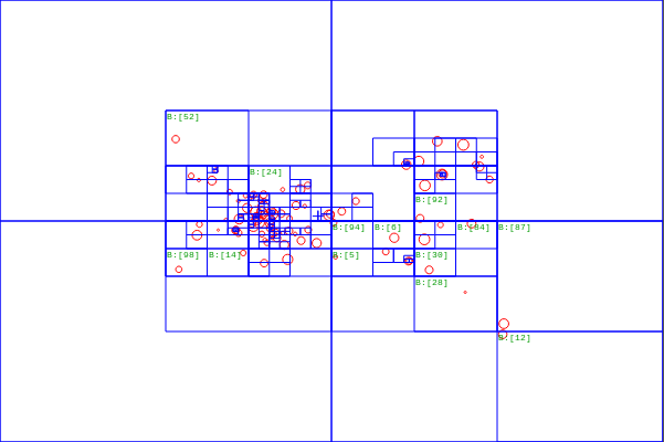
Each node is divided into cubes recursively until only one particle is left and the algorithm
stops (Figure (1)).

Paralellization: In order to perform calculations, GADGET distributes the volume
of the simulation all over the processors of the computer in a Peano-Hilbert
curve 2005MNRAS.364.1105S. This curve carries all particle information and divides it
gradually in the processors which allows an equally distributed load.
Force interaction computation: For each particle, the Tree-PM algorithm produces a branch
from the computer root. In this case, the root is the main node and behaves as a mesh that
spreads on the next nodes. If the current node is at a smaller distance from the particle at
which the calculation is being made, then the node is added to an interaction list.
If, on the other hand, the centre of mass of the node is at a greater distance from the particle, then the node opens and the following question is made: Is the distance of the centre of mass of the mesh greater than the size of the initial cube divided by some parameter, say ? In other words, the question is whether the following relation is fulfilled
| (28) |
where is the distance of the particle to the centre of mass of the mesh, is the size of the initial cube and is a precision parameter. If the expression (28) is true for every particle in the simulation, it continues evolving; on the other hand, if one or more particles do not satisfy this relation, the initial cube is divided into a smaller cube of size and the process is repeated. The algorithm computes multipole expansions and allocate the centre of mass of each cube. After that the question is asked again for each process (Figure 1).
Alternatively, the SPH method for cosmological simulations is mainly used for modelling the interstellar medium and uses the information obtained previously from the force interaction, like the nearest neighbours list to the particle and the force between them. By doing so, the computing time is drastically reduced by avoiding loop calculations.
2.5 GADGET-2 Installation
GADGET-2 is a free source code, ready to download and use it for making simulations.
The instructions to compile and run the code may depend on the operating system that is being used;
if the user has a Lunix or UNIX based system, the compilation is very straightforward.
In the case of a MacOS user,
an Xcode update is needed, which includes all necessary compilation tools to install the code.
For a Windows system, the environment Cygwin is required to use any UNIX based
compilation system.
The following software is required:
- 1.
Gadget-2.0.7.
- 2.
A 1.9 or higher version of GNU scientific library (GSL).
- 3.
The 2.1.5 version of FFTW fast Fourier Transform in the West.
- 4.
A parallel processing library, like Message Passing Interface (MPI) or OpenMPI or MPICH.
- 5.
THe HDF format library dependencies Hierarchical Data Format, versión 1.6.10.
The parallel processing libraries can be directly installed on a Linux based system. The OpenMPI package comes within the MacOS systems. On a side note, DO NOT download any 3.x version of FFTW, because it does not support parallel processing.
Once the software is downloaded, proceed to unzip the .tar.gz file and install. The following process is made on a Linux terminal, so be aware of that:
- 1.
Extract the software:
user@PC/Documents/code: tar -xzvf fftw-2.1.5.tar.gz
user@PC/Documents/code: tar -xzvf gsl-1.9.tar.gz
user@PC/Documents/code: tar -xzvf gadget-2.0.7.tar.gz
user@PC/Documents/code: tar -xzvf hdf5-1.6.10.tar.gz
- 2.
Install GSL: user@PC/Documents/code: cd gsl-1.9/
user@PC/Documents/code/gsl-1.9: ./configure
user@PC/Documents/code/gsl-1.9: make
user@PC/Documents/code/gsl-1.9: sudo make install
This is a root installation. It may depend on the computer manager to give admin privileges to the user or in other case, to install it on another folder, making sure the path to the necessary libraries is correct.
--prefix=/path/to/folder/
- 3.
Install FFTW:
user@PC/Documents/code: cd fftw-2.1.5
user@PC/Documents/code/fftw-2.1.5: ./configure - -enable-mpi - -enable-type-prefix - -enable-float
user@PC/Documents/code/fftw-2.1.5: make
This step takes roughly 10 minutes, so feel free to go for a coffee or a snack. Finally, install the libraries as root:
user@PC/Documents/code/fftw-2.1.5: sudo make install
- 4.
Install the HDF library:
user@PC/Documents/code: cd hdf5-1.6.10
user@PC/Documents/code/hdf5-1.6.10: ./configure
user@PC/Documents/code/hdf5-1.6.10: sudo make install
- 5.
Edit the Gadget Makefile:
This code has a wide variety of parameters to compile which are richly described on the User’s guide. Inside the Gadget’s compile folder go to the Gadget-2 folder and open the Makefile in a terminal or a notepad, then edit the Makefile to follow the path where the GSL and FFTW libraries were installed:
#-------Adjust settings for target computer
.................
#HDF5INCL =
#HDF5LIB  =  -lhdf5 -lz
endif
By default, the libraries are located in /usr/local/. The installation of Gadget in a computational cluster is a little bit tricky, please take a look to this document made by HPC Advisory Council11 1 www.hpcadvisorycouncil.com/pdf/GADGET-2_Best_Practices.pdf. The Makefile has to be edited depending on the system that will be simulated.
3 Examples
Before executing any simulation, the Makefile inside the Gadget-2 folder needs to be edited. These two following examples are two different systems: a) two colliding disk galaxies and b) the large scale structure formation in a CDM Universe; and they were run in a 4-cpu computer.
3.1 Colliding galaxies
This simulation consists of two disk galaxies approaching each other, leading to a fusion between them. Each galaxy has a stellar disk and a dark matter halo using Newtonian Physics, with 20,000 disk particles and 40,000 dark matter halos (Figure 2). For this example, the following lines of the Makefile are modified:
#--------------------------------------- Basic operation mode of code
#OPT   +=  -DPERIODIC
OPT   +=  -DUNEQUALSOFTENINGS

#--------------------------------------- Things that are always recommended
OPT   +=  -DPEANOHILBERT
OPT   +=  -DWALLCLOCK

#--------------------------------------- TreePM Options
#OPT   +=  -DPMGRID=256
..................
The rest of the file remains the same. To run this simulation, it is highly recommended to make a new working folder with the parameter files and executables in order to avoid eventual troubles because of reediting the Makefile
user@PC/Documents/code/Gadget-2.0.7: mkdir galaxy
Then, copy the .exe file in the galaxy folder:
user@PC/Documents/code/Gadget-2.0.7: cp Gadget2/Gadget2 galaxy/
The parameter files have all the information that the simulation needs to run: the particle number,
the initial conditions and so on. This file is inside the parameterfiles folder,
make sure to copy them to the galaxy folder:
user@PC/Documents/code/Gadget-2.0.7: cp Gadget2/parameterfiles/
galaxy.param galaxy/
Now, edit the default parameter file named galaxy.param
user@PC/Documents/code/Gadget-2.0.7: cd galaxy
The two first lines have to look as follow:
% Relevant files

InitCondFile /path/to/Gadget-2.0.7/ICs/galaxy_littleendian.dat
OutputDir /path/to/Gadget-2.0.7/galaxy/
where path/to/Gadget-2/ICs and path/to/Gadget-2/galaxy are the paths
where the Initial conditions are being read and where the output files want to be created.
Now all is set to run the first collision simulation:
user@PC/Documents/code/Gadget-2.0.7/galaxy: mpirun -np 2 ./Gadget2 galaxy.param
This line calls for an MPI script to parallel processing. The -np 2 indicates how many processors will be used for the computation.


3.2 Large scale structure formation
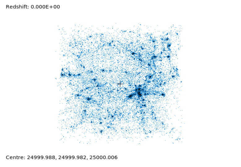
This is an example of dark matter particles and gas particles. The structure formation is made within a periodic box of size per side in a CDM Universe (Figure 3). This simulation distributes the particles in a cubic mesh, where they are placed in the mesh centres surrounded by dark matter particles. A perturbation on the position makes the particles move and eventually they form structures. The code starts running from and finishes at the present epoch (). The parameters of this simulation are indicated in Table 1.
| Description | Symbol | Value |
|---|---|---|
| Dark matter density | 0.3 | |
| Dark energy density | 0.7 | |
| Baryonic matter density | 0.04 | |
| Hubble parameter | 0.7 | |
| ( ) |
The Gadget Makefile needs to be edited as follows:
#--------------------------- Basic operation mode of code
OPT   +=  -DPERIODIC
#OPT   +=  -DUNEQUALSOFTENINGS

#------------------------------- Things that are always recommended
OPT   +=  -DPEANOHILBERT
OPT   +=  -DWALLCLOCK

#----------------------------------------- TreePM Options
OPT   +=  -DPMGRID=128
......................
To run the software it is necessary to call the parameters file lcdm_gas.param.
A variety of codes to generate initial conditions for large scale structure formation exists,
these codes use Lagrangian Perturbation theory (LPT) such as the Zeldovich Approximation (ZA).
For this example, the initial conditions were created using the N-GenIC software which
can be easily manipulated. To run the code, just execute it as follows:
user@PC/Documents/code/Gadget-2.0.7/lcdm_gas: mpirun -np 2/ ./Gadget2 lcdm_gas.param
This example takes roughly 20 minutes to finish. This is because the number of particles simulated are just a few compared to a major resolution simulation, in which case it needs to be executed on a computational cluster.


4 Creating initial conditions
GADGET is a code that evolves a system of particles, the initial conditions need to be created using other codes and resources such as GalIC 2014MNRAS.444…62Y and N-GenIC 2009MNRAS.394.1559G, to create initial conditions for galaxies and large structures respectively. Other codes can also be used for such purposes, as MusIC 2011MNRAS.415.2101H and 2LPTIC 2006MNRAS.373..369C that use a Second Order Lagrangian Perturbation Theory.
4.1 GalIC
This code uses an iterative method to compute -body simulations in equilibrium systems given its density distributions, such as spherically symmetric functions, axisymmetrical systems and galaxy models with different density profiles. There are two versions of GalIC, the galic 1.0 version and the galic 1.1 version. The installation of the first version is quite similar to installing GADGET. For the 1.1 version, it is also necessary a Doxygen tool, because this version is intended to be more accessible to another operating systems and programming languages.
The folder includes a list of examples listed on Table 1 of reference 2014MNRAS.444…62Y, and the parameters may be changed to make major resolution simulations.
4.2 N-GenIC
This code uses the Zeldóvich Approximation 1970A&A…..5…84Z; RevModPhys.61.185, which describes a non-linear evolution of the state of a matter density gravitational perturbation, which is considered to be homogeneous and non-collisional. In the file, the following parameters can be edited:
- 1.
Simulation including either only dark matter or dark matter with gas particles.
- 2.
The number of particles .
- 3.
The initial time of the simulation .
- 4.
Dark matter density ().
- 5.
Dark energy density ().
- 6.
Baryonic matter density ().
- 7.
Hubble’s parameter ().
- 8.
Boxsize of the simulation ().
- 9.
Power spectrum normalization () 1993MNRAS.262.1023W.
5 Results
Using the parameters of Table 2, a structure formation simulation was carried out starting from to in a CDM Universe. On the other hand, the matter power spectrum was generated with the code CAMB 2000ApJ…538..473L, and compared with the outcome from the simulation (see Figure 5).
| Description | Symbol | Value | |
| Densities at | Dark matter | 0.268 | |
| Dark energy | 0.683 | ||
| Baryonic matter | 0.049 | ||
| Simulation | Boxsize | 50 Mpc | |
| No. of particles | 4096 | ||
| Redshift | Initial | 23 | |
| Final | 0 | ||
| Other quantities | Hubble’s parameter | 0.7 | |
| Matter power spectrum normalisation | 0.8 |
| Description | Quantity | Units | |
|---|---|---|---|
| Unit system | Length(cm) | 1 kpc | |
| Masa (g) | |||
| Velocity (cm/s) | 1 km/s | ||
| Softening | CDM() | 0.89, 20 | kpc |


To compute the mater power spectrum generated by the simulation, the code POWMES 2009MNRAS.393..511C comes in handy because it is designed to estimate the power spectrum of -body simulations in an iterative form. The power spectrum characterises the scales and clustering of galaxies in the Universe. In particular, many cosmological constrictions are based on the measurement or its inverse Fourier transform, the two point correlation function.
Figure (5) shows the matter power spectrum computed by CAMB which is very close to the non-linear regime ( indicates large scales) with a softening value of kpc. The similarities are visible when comparing the solution of the Boltzmann equations and the numerical solution via the CDM simulation. As expected, the number of particles does affect the final result of the simulation; less particles lead to low matter power spectrum compared to the rest of the spectra, as well as to the one computed by CAMB. It is also visible that when the softening parameter increases the simulation creates less structure, because is preventing the particles to come closer than 2 kpc. These are important parameters to bear in mind, as they need to be selected very carefully and effectively to get accurate results. The simple difference of one parameter can affect the whole result.
6 Conclusions and future work
In this work we present a general description of the dark matter enigma, its discovery, and incorporation into the standard cosmological CDM model. The model has been successfully tested through several observations, and compared with numerical simulations, in particular simulations at small scales where dark matter halos in galaxies are formed due to a spherical collapse model and on large scales by studying the cluster formation.
-body simulations have been used in the cosmology field as an efficient tool to study process of large scale structure formation in the Universe. In this scheme, dark matter is modelled as a non-collisional fluid under the influence of a gravitational potential. Other models such as the SPH method involve gas dynamics for galaxy formation. Using these two methods, the interaction between dark matter particles and gas particles can be observed via the accretion of the gas into the dark matter halos. In this work, GADGET was used as a main code for simulating the large scale structure of a 50 Mpc Box in a CDM Universe. The installation process of GADGET is also mentioned as an effective and simple guide to follow for young scientists.
The many parameters of an -body code can be easily modified, and variations of them can lead to a whole new physical system on the simulation. Thus it is important to test the various parameters and theories with a well established method (like the analytical solution to the Boltzmann equations) and then compare the variation of the parameters of the simulation. In this work, we performed different tests on various parameters which led to similar results predicted from an analytic CDM model, but a variation on the number of particles as well as the softening length led to different results. It is also important to highlight the key role that the gravitational softening plays on the simulations, different softening may recreate systems that resemble observations in different surveys.
The data analysis requires the knowledge of statistical and probabilistic methods, and density distributions often studied in cosmology. Nevertheless, there exists some details within the structure formation theory that lead to issues in both observations and simulations, these issues are primarily the CUSP-CORE problem and the missing satellite problem. There are different alternatives to solve them, however, one of the main approaches in future work will be to compare different models to CDM using different codes and initial conditions adapted for each one.
Several numerical codes were discussed, such as Tree, Particle-mesh, AMR and so on, listing their characteristics and differences. These codes are used for modelling diverse astrophysical systems, in particular, the -body approach is used for galactic and cosmological systems, mainly governed by the non-collisional Boltzmann equations. The code N-GenIC comes very handy for generating initial conditions without gas particles, this software will be very useful to compare a GADGET modification which uses an axion model for dark matter particles called Axion-GADGET 2018ApJ…853…51Z. With this model, the main goal is to provide an alternative solution to several issues the CDM model is dealing with, such as the CUSP-CORE problem 1996ApJ…462..563N; 1997ApJ…490..493N; Moore:1994yx observed on the density distribution of many galaxies and the missing satellite problem 1999MNRAS.310.1147M; 2005Natur.435..629S. This modification continues in development and we are aiming to improve the short range interaction between systems.
Acknowledgments
J.A.V. acknowledges FOSEC SEP-CONACYT Investigación Básica A1-S-21925 and UNAM-DGAPA-PAPIIT IA102219.
References
- (1) B. Ryden, Introduction to cosmology. 2003.
- (2) D. N. Spergel, R. Bean, O. Doré, M. R. Nolta, C. L. Bennett, J. Dunkley, G. Hinshaw, N. Jarosik, E. Komatsu, L. Page, H. V. Peiris, L. Verde, M. Halpern, R. S. Hill, A. Kogut, M. Limon, S. S. Meyer, N. Odegard, G. S. Tucker, J. L. Weiland, E. Wollack, and E. L. Wright, “Three-Year Wilkinson Microwave Anisotropy Probe (WMAP) Observations: Implications for Cosmology,” ApJS, vol. 170, pp. 377–408, June 2007.
- (3) J. C. Mather, E. S. Cheng, D. A. Cottingham, R. E. Eplee, Jr., D. J. Fixsen, T. Hewagama, R. B. Isaacman, K. A. Jensen, S. S. Meyer, P. D. Noerdlinger, S. M. Read, L. P. Rosen, R. A. Shafer, E. L. Wright, C. L. Bennett, N. W. Boggess, M. G. Hauser, T. Kelsall, S. H. Moseley, Jr., R. F. Silverberg, G. F. Smoot, R. Weiss, and D. T. Wilkinson, “Measurement of the cosmic microwave background spectrum by the COBE FIRAS instrument,” ApJ, vol. 420, pp. 439–444, Jan. 1994.
- (4) F. Zwicky, “On the Masses of Nebulae and of Clusters of Nebulae,” ApJ, vol. 86, p. 217, Oct. 1937.
- (5) V. C. Rubin and W. K. Ford, Jr., “Rotation of the Andromeda Nebula from a Spectroscopic Survey of Emission Regions,” ApJ, vol. 159, p. 379, Feb. 1970.
- (6) A. A. Penzias and R. W. Wilson, “A Measurement of Excess Antenna Temperature at 4080 Mc/s.,” ApJ, vol. 142, pp. 419–421, July 1965.
- (7) M. R. Blanton, M. A. Bershady, B. Abolfathi, F. D. Albareti, C. Allende Prieto, A. Almeida, J. Alonso-García, F. Anders, S. F. Anderson, B. Andrews, and et al., “Sloan Digital Sky Survey IV: Mapping the Milky Way, Nearby Galaxies, and the Distant Universe,” AJ, vol. 154, p. 28, July 2017.
- (8) B. Schutz, A First Course in General Relativity. Cambridge University Press, 2nd ed., June 2009.
- (9) E. Hubble, “A Relation between Distance and Radial Velocity among Extra-Galactic Nebulae,” Proceedings of the National Academy of Science, vol. 15, pp. 168–173, Mar. 1929.
- (10) N. Mandolesi, C. Burigana, A. Gruppuso, and P. Natoli, “The Planck Mission: Recent Results, Cosmological and Fundamental Physics Perspectives,” International Journal of Modern Physics D, vol. 22, p. 1330029, Dec. 2013.
- (11) P. J. E. Peebles, Principles of Physical Cosmology. 1993.
- (12) M. Sasaki, “Large Scale Quantum Fluctuations in the Inflationary Universe,” Progress of Theoretical Physics, vol. 76, pp. 1036–1046, 11 1986.
- (13) A. H. Guth, “Inflationary universe: A possible solution to the horizon and flatness problems,” Phys. Rev. D, vol. 23, pp. 347–356, Jan. 1981.
- (14) P. J. Peebles and B. Ratra, “The cosmological constant and dark energy,” Reviews of Modern Physics, vol. 75, pp. 559–606, Apr. 2003.
- (15) J. F. Navarro, C. S. Frenk, and S. D. M. White, “The Structure of Cold Dark Matter Halos,” ApJ, vol. 462, p. 563, May 1996.
- (16) J. F. Navarro, C. S. Frenk, and S. D. M. White, “A Universal Density Profile from Hierarchical Clustering,” ApJ, vol. 490, pp. 493–508, Dec. 1997.
- (17) B. Moore, “Evidence against dissipationless dark matter from observations of galaxy haloes,” Nature, vol. 370, p. 629, 1994.
- (18) B. Moore, T. Quinn, F. Governato, J. Stadel, and G. Lake, “Cold collapse and the core catastrophe,” MNRAS, vol. 310, pp. 1147–1152, Dec. 1999.
- (19) V. Springel, S. D. M. White, A. Jenkins, C. S. Frenk, N. Yoshida, L. Gao, J. Navarro, R. Thacker, D. Croton, J. Helly, J. A. Peacock, S. Cole, P. Thomas, H. Couchman, A. Evrard, J. Colberg, and F. Pearce, “Simulations of the formation, evolution and clustering of galaxies and quasars,” Nature, vol. 435, pp. 629–636, June 2005.
- (20) T. Matos, A. Vazquez-Gonzalez, and J. Magana, “ as Dark Matter,” Mon. Not. Roy. Astron. Soc., vol. 393, pp. 1359–1369, 2009.
- (21) J. Magana and T. Matos, “A brief Review of the Scalar Field Dark Matter model,” J. Phys. Conf. Ser., vol. 378, p. 012012, 2012.
- (22) L. Hui, J. P. Ostriker, S. Tremaine, and E. Witten, “Ultralight scalars as cosmological dark matter,” Phys. Rev. D, vol. 95, no. 4, p. 043541, 2017.
- (23) S. Mikkola and S. J. Aarseth, “An implementation ofn-body chain regularization,” Celestial Mechanics and Dynamical Astronomy, vol. 57, pp. 439–459, Nov 1993.
- (24) J. Barnes and P. Hut, “A hierarchical O(N log N) force-calculation algorithm,” Nature, vol. 324, pp. 446–449, Dec. 1986.
- (25) A. Klypin and J. Holtzman, “Particle-mesh code for cosmological simulations,” 1997.
- (26) B. W. O’Shea, G. Bryan, J. Bordner, M. L. Norman, T. Abel, R. Harkness, and A. Kritsuk, “Introducing Enzo, an AMR Cosmology Application,” arXiv Astrophysics e-prints, Mar. 2004.
- (27) V. Springel, “High performance computing and numerical modelling,” 2014.
- (28) J. Chacón, “Modelos de materia oscura: Una perspectiva numérica.” Escuela Superior de Física y Matemáticas, B.S. Thesis, http://pelusa.fis.cinvestav.mx/tmatos/CV/3_RecursosH/Lic/Jazhiel_ESFM.pdf, Dec 2018.
- (29) E. Parzen, “On estimation of a probability density function and mode,” Ann. Math. Statist., vol. 33, pp. 1065–1076, 09 1962.
- (30) R. A. Gingold and J. J. Monaghan, “Smoothed particle hydrodynamics - Theory and application to non-spherical stars,” MNRAS, vol. 181, pp. 375–389, Nov. 1977.
- (31) J. J. Monaghan, “SPH and Riemann Solvers,” Journal of Computational Physics, vol. 136, pp. 298–307, Sept. 1997.
- (32) J. J. Monaghan, “Smoothed particle hydrodynamics,” ARA&A, vol. 30, pp. 543–574, 1992.
- (33) V. Springel, “The cosmological simulation code GADGET-2,” MNRAS, vol. 364, pp. 1105–1134, Dec. 2005.
- (34) J. J. Monaghan and J. C. Lattanzio, “A refined particle method for astrophysical problems,” A&A, vol. 149, pp. 135–143, Aug. 1985.
- (35) P. Bodenheimer, G. P. Laughlin, M. Rozyczka, and H. W. Yorke, eds., Numerical Methods in Astrophysics: An Introduction, 2007.
- (36) D. Yurin and V. Springel, “An iterative method for the construction of N-body galaxy models in collisionless equilibrium,” MNRAS, vol. 444, pp. 62–79, Oct. 2014.
- (37) M. Grossi and V. Springel, “The impact of early dark energy on non-linear structure formation,” MNRAS, vol. 394, pp. 1559–1574, Apr. 2009.
- (38) O. Hahn and T. Abel, “Multi-scale initial conditions for cosmological simulations,” MNRAS, vol. 415, pp. 2101–2121, Aug. 2011.
- (39) M. Crocce, S. Pueblas, and R. Scoccimarro, “Transients from initial conditions in cosmological simulations,” MNRAS, vol. 373, pp. 369–381, Nov 2006.
- (40) Y. B. Zel’dovich, “Gravitational instability: An approximate theory for large density perturbations.,” A&A, vol. 5, pp. 84–89, Mar. 1970.
- (41) S. F. Shandarin and Y. B. Zeldovich, “The large-scale structure of the universe: Turbulence, intermittency, structures in a self-gravitating medium,” Rev. Mod. Phys., vol. 61, pp. 185–220, Apr 1989.
- (42) S. D. M. White, G. Efstathiou, and C. S. Frenk, “The amplitude of mass fluctuations in the universe,” MNRAS, vol. 262, pp. 1023–1028, June 1993.
- (43) A. Lewis, A. Challinor, and A. Lasenby, “Efficient Computation of Cosmic Microwave Background Anisotropies in Closed Friedmann-Robertson-Walker Models,” ApJ, vol. 538, pp. 473–476, Aug 2000.
- (44) S. Colombi, A. Jaffe, D. Novikov, and C. Pichon, “Accurate estimators of power spectra in N-body simulations,” MNRAS, vol. 393, pp. 511–526, Feb. 2009.
- (45) J. Zhang, Y.-L. Sming Tsai, J.-L. Kuo, K. Cheung, and M.-C. Chu, “Ultralight Axion Dark Matter and Its Impact on Dark Halo Structure in N-body Simulations,” ApJ, vol. 853, p. 51, Jan 2018.