Adaptive Spectral Decompositions
For Inverse Medium Problems
Abstract
Inverse medium problems involve the reconstruction of a spatially varying unknown medium from available observations by exploring a restricted search space of possible solutions. Standard grid-based representations are very general but all too often computationally prohibitive due to the high dimension of the search space. Adaptive spectral (AS) decompositions instead expand the unknown medium in a basis of eigenfunctions of a judicious elliptic operator, which depends itself on the medium. Here the AS decomposition is combined with a standard inexact Newton-type method for the solution of time-harmonic scattering problems governed by the Helmholtz equation. By repeatedly adapting both the eigenfunction basis and its dimension, the resulting adaptive spectral inversion (ASI) method substantially reduces the dimension of the search space during the nonlinear optimization. Rigorous estimates of the AS decomposition are proved for a general piecewise constant medium. Numerical results illustrate the accuracy and efficiency of the ASI method for time-harmonic inverse scattering problems, including a salt dome model from geophysics.
Keywords: Adaptive eigenspace inversion, AEI, full waveform inversion, inverse scattering problem, total variation regularization
1 Introduction
Inverse medium problems occur in a wide range of applications such as medical imaging, geophysical exploration and non-destructive testing. Given observations of a physical state variable, , from the boundary of a bounded region , one seeks to reconstruct (unknown) spatially varying medium properties, , inside . In inverse scattering problems, for instance, characterizes the location, shape or physical properties of the scatterer, typically a collection of bounded or penetrable inclusions, while the scattered wave field satisfies the governing (time-dependent or time-harmonic) wave equation. In seismic imaging, in particular, full-waveform inversion reconstructs high-resolution subsurface models of the medium parameters (e.g. spatially varying sound speed) from reflected seismic waves at the Earth’s surface [27]. To determine from boundary measurements of , the inverse medium problem is usually reformulated as a PDE-constrained optimization problem for a cost functional , which measures the misfit between the simulated and the observed data [30, 19].
Two difficulties one must address when solving an inverse medium problem numerically are the well-posedness of the problem and the size of the set of candidate functions for . It is well-known that the problem of minimizing the misfit over is, in general, ill-posed. To obtain a well-posed problem, the misfit functional is typically modified by adding a Tikhonov-type regularization term [31, 11]. Then the resulting formulation may be discretized and solved numerically [25, 17]. Although Tikhonov regularization generally improves the stability of the inversion, it does not address the cost of solving an optimization problem in a subspace of high dimension, still determined by the number of degrees of freedom of the spatial numerical discretization.
When a parametrization of the unknown medium is explicitly known a priori, the inversion can easily be limited to a reduced set of unknown parameters. Moreover, if the search space is of sufficiently low dimension, the discretization itself can have a regularizing effect [4, 22]. In general, however, such a low-dimensional representation is not explicitly known a priori.
To resolve the vexing dilemma of remaining sufficiently general while keeping the dimension of the search space sufficiently small, various sparsity promoting strategies were proposed in recent years. In [6], Daubechies, Defrise and De Mol considered linear inverse problems yet replaced the usual quadratic regularizing penalty by weighted -penalties on the coefficients to promote a sparse expansion of with respect to an orthonormal basis. Later, Loris et al. [24] successfully applied -norm soft-thresholding to promote a sparse wavelet representation of for seismic tomography. Similarly, a truncated wavelet representation of the acoustic velocity and mass density was used for seismic FWI in [23]. In [20], a curvelet-based representation of the wave field was used for seismic data recovery from a regularly sampled grid with traces missing. Recently, Kadu, van Leeuwen and Mulder [21] combined a level-set representation, constructed from radial basis functions, with a Gauss-Newton approximation to regularize FWI in the presence of salt bodies.
In [9], de Buhan and Osses proposed to restrict the search space to the span of a small basis of eigenfunctions of a judicious elliptic operator, repeatedly adapted during the nonlinear iteration. Their approach relies on a decomposition
| (1.1) |
for functions . Here satisfies the elliptic boundary-value problem
| (1.2) |
and for , each is an eigenfunction of a -dependent, linear, symmetric, and elliptic operator , that is, satisfies
| (1.3) |
for an eigenvalue . The eigenvalues form a nondecreasing sequence, with each eigenvalue repeated according to its multiplicity, and the set is an orthonormal basis of . Henceforth we shall refer to (1.1) as the adaptive spectral (AS) expansion or decomposition.
The AS decomposition has been used in various iterative Newton-like inversion algorithms [8, 16, 18] as follows: Given an approximation of the medium, , from the previous iteration, the approximation at the current iteration is set as the minimizer of the misfit functional in the affine space , where and , , satisfy (1.2) and (1.3) with , respectively. As the approximation changes from one iteration to the next, so does the affine search space used for the subsequent minimization.
Clearly, the choice of is crucial in obtaining an efficient approximation of the medium with as few basis functions as possible. The particular choice for used in [9], which essentially coincides with the linearization of the gradient of the penalized total variation (TV) functional [16], yields a remarkably efficient approximation for piecewise constant functions. Although is not well-defined for piecewise constant , numerical discretizations of (1.2) or (1.3) can be viewed as approximations with replaced by a more regular approximation of , such as a projection of on an -conforming finite element (FE) space. The AS decomposition also bears a striking similarity to nonlinear eigenproblems for the (subdifferential of the) TV functional and, more generally, for one homogeneous functionals used in image processing – see [3, 5, 1] and the references therein. Depending on a priori available information about the smoothness or spatial anisotropy of the medium, different choices for will yield more or less efficient AS representations [18].
By combining the adaptive inversion process with the TRAC (time reversed absorbing condition) approach, de Buhan and Kray [8] developed an effective solution strategy for time-dependent inverse scattering problems. In [16], Grote, Kray and Nahum proposed the AEI (adaptive eigenspace inversion) algorithm for inverse scattering problems in the frequency domain. It combines the AS decomposition with frequency stepping and truncated inexact Newton-like methods [28, 25], and may also be used without Tikhonov regularization by progressively increasing the dimension of the spectral basis with frequency. In [18], the AEI algorithm was extended to multi-parameter inverse medium problems, including the well-known layered Marmousi subsurface model from geosciences. Recently, it was extended to electromagnetic inverse scattering problems at fixed frequency [7] and also to time-dependent inverse scattering problems when the illuminating source is unknown [15].
So far, the remarkable efficiency and accuracy of the AS decomposition for the approximation of piecewise constant functions is only justified via numerical evidence. Although previous inversion algorithms based on the AS decomposition iteratively adapt the basis functions , they do not provide any criteria for adapting the dimension of the search space. Here, we precisely address these two open questions. In Section 2, we present a strategy for adapting the dimension of the search space, by solving a small quadratically constrained quadratic minimization problem to filter basis functions while preserving important features. The resulting new ASI (adaptive spectral inversion) algorithm is listed in Section 2.2. In Section 3, we derive rigorous error estimates for and for the first eigenvalues and eigenfunctions of the elliptic operator associated with a piecewise constant function. In particular, we prove that and the first eigenfunctions are “almost” piecewise constant in the sense that their gradients are small outside a neighborhood of internal discontinuities. We also provide a numerical example which illustrates the theory. In Section 4, we apply the ASI Algorithm to two inverse medium problems, the first where the medium is composed of five simple geometric inclusions, and the second, where the medium corresponds to a two-dimensional model of a salt dome from geophysics. Finally, we conclude with some remarks in Section 5.
2 Inverse scattering problem
First, we consider a time-harmonic inverse scattering problem and reformulate it as a PDE-constrained optimization problem. Then we present the adaptive spectral inversion (ASI) method, list the full ASI Algorithm and discuss in further detail the individual steps in adapting both the basis and its dimension during the nonlinear iteration.
2.1 Inverse scattering problem
We consider a time-harmonic inverse scattering problem where the scattered wave field, , satisfies the Helmholtz equation:
| (2.1a) | ||||||
| (2.1b) | ||||||
Here, is a bounded domain with Lipschitz boundary and outward unit normal , and are known sources, and is the angular frequency corresponding to the (regular) frequency . The squared wave speed, , of the (unknown) medium satisfies throughout and is assumed known on the boundary .
Given observations on a subset of of the scattered fields, , due to known sources and , , we wish to recover the medium inside by minimizing the cost functional ,
| (2.2) |
Hence, we consider the PDE-constrained optimization problem,
| (2.3) |
where is a space of candidate media and solves (2.1) with and . We regard as a subspace of with its standard inner product and norm, denoted by and , respectively.
2.2 Adaptive spectral inversion
The adaptive spectral inversion (ASI) algorithm minimizes in (2.2) over a finite-dimensional subspace of by building and repeatedly adapting a finite basis as follows. Suppose we have, at iteration , a function , which coincides with the true medium on the boundary, and a subspace spanned by an orthonormal set
| (2.4) |
of functions that vanish on . Then, we determine a (local) minimizer of in the -dimensional affine space , i.e.,
| (2.5) |
using any standard Newton or quasi-Newton method; the smaller , the cheaper the numerical solution of the nonlinear optimization problem (2.5).
Once we have determined , we must update the search space needed at the next iteration, that is, determine and . First, we compute , by solving
| (2.6) |
where is a -dependent, symmetric and elliptic operator; the particular form used here is specified below, but other choices are possible – see Section 3 and [18]. Recall that is assumed known on the boundary . Then, we compute the first (orthonormal) eigenfunctions of (or possibly , cf. [16, 18]) by solving the eigenvalue problem
| (2.7) |
for the smallest, not necessarily distinct eigenvalues . The eigenfunctions should enable an efficient representation of the current iterate but also enrich the search space by introducing new potential candidate media for further minimizing at the next iteration.
Next, we merge the current search space with the space spanned by the new eigenfunctions as
| (2.8) |
to ensure that the current solution also belongs to . By a standard Gram-Schmidt procedure, we compute an -orthonormal basis for the merged space,
In the process of adapting the search space, it is crucial to also adapt its new dimension, which not only directly impacts the computational cost but also acts as regularization. Hence, we shall reduce and thus obtain the new search space of dimension while imposing some regularity on the solution. To decide which basis functions of to keep and which to discard, we compute an indicator as a filtered approximation of in . Then, we reorder the basis functions in decreasing order of its Fourier coefficients
| (2.9) |
and discard any associated with small . This yields the new search space spanned by the remaining basis functions,
| (2.10) |
Below we summarize the entire adaptive spectral inversion (ASI) Algorithm:
In the above ASI Algorithm, most of the computational work occurs in Step 1, which involves multiple numerical solutions of the (forward) problem (2.1). For (2.6) and (2.7) in Step 1, we always use of the form
| (2.11) |
where the -dependent weight function is given by
| (2.12) |
with a small parameter; in our computations, we always set . Note that the theoretical properties of the adaptive spectral decomposition proved in Section 3 also apply to more general . We now describe in more detail the individual steps of the above ASI Algorithm.
To initialize the ASI Algorithm, we require an initial guess , an approximation of the background that coincides with the medium on the boundary, and a finite dimensional space given as the span of an orthonormal basis
The initial background and orthonormal basis of can be determined by solving (2.6) and (2.7) with and setting . For instance, if is constant throughout and equal to on the boundary, then whereas correspond to the first eigenfunctions of the Laplacian. Alternatively, one may choose or the basis of a priori, independently of .
For the minimization of (2.5) in Step 1, we opt for a quasi-Newton method with rank-two updates (BFGS, [26]), but other choices are possible. As initial guess for , one can use the -projection onto either of or its filtered approximation .
In Step 1, the number of new eigenfunctions is somewhat arbitrary, since the dimension of the new basis is anyway adapted subsequently; here, we typically take with . To obtain the -orthonormal basis for in Step 1, we apply the standard modified Gram-Schmidt algorithm to the ordered set
spanning .
In Step 1, we compute the indicator used subsequently for truncating the space as follows. The basis of the truncated new search space ought to preserve edges in the medium but also suppress noise. Hence, we seek an indicator which is close to , yet with minimal TV, by considering the constrained minimization problem
| (2.13) | ||||
for a prescribed tolerance . Since the solution of (2.13) is expensive, we replace the TV functional
| (2.14) |
Hence, we compute the indicator by solving the quadratically constrained quadratic minimization problem for fixed ,
| (2.15) | ||||
which is cheap.
Once has been computed, we truncate in Step 1 as follows. Given the Fourier coefficients of arranged in decreasing order, with as in (2.9), we remove the maximal number of basis functions with corresponding smallest Fourier coefficients, setting
| (2.16) |
for a given tolerance . To avoid abrupt changes in the number of basis functions from one iteration to the next, we accept the value without further change if
| (2.17) |
for some prescribed . Otherwise if , we still set but also increase , e.g., by doubling it, to avoid such an overly large increase in dimension at the next iteration. On the other hand if , we set to avoid an overly rapid drop in dimension and thus lose important information; moreover, we decrease in (2.16), e.g., by halving it. Typically, we choose , , and .
Finally, we embed the ASI algorithm in a standard frequency stepping approach, where the inverse problem is solved at increasingly higher frequencies . Whenever two consecutive iterates satisfy
| (2.18) |
for a given tolerance , we proceed to the observations obtained at a higher frequency.
3 Analysis of adaptive spectral decompositions
In this section we derive estimates for and the eigenvalues and eigenfunctions of the linear operator defined in (2.11) with an -regular approximation of a given piecewise constant function . Typically, the medium-dependent weight function which characterizes the AS decomposition has either the form
| (3.1) |
for some , or
| (3.2) |
For the analysis below, we allow to have a more general form.
3.1 Assumptions and definitions
3.1.1 Medium dependent weight function
Let be a bounded and connected Lipschitz domain. We assume that for , with , is given by
| (3.3) |
where is a non-increasing function that satisfies
| (3.4) |
In particular, these assumptions yield
| (3.5) |
and
| (3.6) |
Although this framework encompasses weight functions as in (3.1) or (3.2), it does not include weight functions, associated with the Lorentzian or Gaussian penalty terms [18], for instance, which do not satisfy the last inequality of (3.4). However, the above framework easily extends to more general weight functions that satisfy an estimate
| (3.7) |
for some . This extension, indeed, addresses the Lorentzian and Gaussian weight functions which satisfy (3.7) with . For the analysis, we assume (3.4), i.e., (3.7) with , and comment on the extension to the more general case in Remark 8 below.
3.1.2 Elliptic boundary value problems
To include FE approximations in the analysis, we formulate the boundary value problems (1.2) and (1.3) in closed subspaces and , respectively. We say that satisfies
| (3.8) |
in , if
| (3.9a) | ||||
| (3.9b) | ||||
where is the bilinear form given by
| (3.10) |
with denoting the standard inner product. We say that is an eigenvalue of in , if there exists such that
| (3.11) |
in , that is, if
| (3.12) |
As shown below, the operator is symmetric and uniformly elliptic. Thus, we let be the nondecreasing (perhaps finite) sequence of (real positive) eigenvalues of in , with each eigenvalue repeated according to its multiplicity, and be a basis of of corresponding eigenfunctions, orthonormal with respect to the inner product. Finally, we denote by the norm of , and by the -norm.
3.1.3 Piecewise constant medium
Let the medium be piecewise constant admitting a decomposition
| (3.13) |
into a piecewise constant background , composed of features reaching the boundary , and a piecewise constant perturbation , composed of a finite number of inclusions separated from the boundary. More precisely, we assume
| (3.14) |
where , and are the characteristic functions of mutually disjoint connected open sets such that
| (3.15) |
where denotes the -dimensional Hausdorff measure. Although the coefficients must satisfy for the Helmholtz equation, they may take any real value in the present analysis. We further assume that
| (3.16) |
where for each , is the characteristic function of a connected open set , where
| (3.17) |
is the set of jump discontinuities, or interfaces, in the background . Moreover, we assume that the sets have mutually disjoint boundaries; the full inclusion of one set inside another, however, is allowed.
For , let denote the -neighborhood of ,
| (3.18) |
and, similarly, let denote the -neighborhood of ,
| (3.19) |
Then we define the open complement as
| (3.20) |
the -interior of as
| (3.21) |
Figure 1 shows a typical arrangement in two dimensions.
Let be an approximation of obtained by a linear method. For example, may be the interpolant of in an -conforming FE space; then, the parameter corresponds to the mesh size. We assume that for each , the approximations of satisfy in , and similarly, for each , that the approximations of satisfy in . For each , the -regular approximation is thus given by
| (3.22) |
where
| (3.23) |
3.2 Statement of main results and discussion
To simplify the presentation, we include in this section only short proofs and proofs of the main results; the remaining proofs are provided in Section 3.3. The main result, given by Theorem 5, provides estimates for the approximation of the background , and for the first eigenvalues and eigenfunctions of in (2.11). From Theorem 5, we deduce Corollary 6 which provides similar estimates for finite element formulations or for obtained from the convolution of with a mollifier.
Theorem 5 relies on Lemmas 2 and 4 which require the approximation of each characteristic function , and , to satisfy
| (3.24) |
for every sufficiently small. Note that since converges to a function with jump discontinuities, the gradients of need not be bounded uniformly with respect to , for close to zero. Whether (3.24) is satisfied depends on geometric properties of the method by which is obtained, as well as on properties of the set . The following lemma provides sufficient conditions for (3.24) to hold.
Lemma 1.
Let be a bounded Lipschitz domain,
with , for , and the Lebesgue measure. Then, the following assertions hold:
- 1.
There exists a constant such that , for every .
- 2.
If such that for all , and if
(3.25) for some (with the usual convention ), then there exists a constant , such that for every ,
(3.26)
In particular, for , (3.25) reduces to a.e. in , for all . Also note that for , the conclusion of the lemma is trivial.
In the following, we assume sufficiently small such that
| (3.27) |
and for each connected component of , there holds . In other words, we assume for , that all -interiors of are non-empty, that all -neighborhoods of the interfaces of the medium, and , do not intersect, and that the only parts of the open complement, , isolated from the boundary are the -interiors of the inclusions . Since the boundaries of are mutually disjoint, and , , such an exists. We further suppose that for each ,
| (3.28a) | |||
| and that for each , | |||
| (3.28b) | |||
These assumptions imply that
| (3.29) |
and
| (3.30) |
By (3.28), for each , , and thus, due to (3.6) with , the operator is uniformly elliptic in , for . A simple but useful conclusion we can draw from (3.30) is
| (3.31) |
For the approximation of the background , we have the following estimate.
Lemma 2.
For every and , there holds
| (3.32) |
The estimates for the eigenfunctions are based on the following simple result.
Proposition 3.
For every and there holds
| (3.33) |
Thus, to show that an eigenfunction is “almost” piecewise constant, we need to estimate the corresponding eigenvalue of in , for which we rely on the following lemma.
Lemma 4.
There exists a constant , independent of and such that for every , , and , there holds
| (3.34) |
Together, the results above yield the following theorem.
Theorem 5.
Let be given by (3.13), the approximation, , of be given by (3.22), be given by (3.9), and with satisfy (3.12), where is non-decreasing and orthonormal in . Suppose and have Lipschitz boundaries, and such that (3.27) is satisfied. If (3.28) hold true, and there exists a constant such that for every , each of the functions , , or , , satisfies
| (3.35) |
then there exists a constant , independent of the coefficients and such that for every and , the following estimates hold:
| (3.36) |
| (3.37) |
Moreover, for each Lipschitz domain with , there exists a constant , independent of the coefficients and such that for every and , the following estimates are satisfied
| (3.38) |
| (3.39) |
Proof.
Essentially, estimates (3.36) and (3.37) imply that and the first eigenfunctions of are “almost” constant in each connected component of . In particular, is almost constant in each connected component of . Since the Hausdorff measure of is positive for each , and coincides with on , indeed approximates well in . Similarly, for , is almost constant in each connected component of and vanishes on ; therefore, every is small in . Consequently, can be well approximated in , for instance, by its -best approximant , where denotes the standard -orthogonal projection
| (3.40) |
Corollary 6.
Proof.
For the proof, it is sufficient to show that in each case (i), (ii), the hypotheses of Theorem 5 are satisfied, i.e., that the approximation of a characteristic function of a Lipschitz domain contained in satisfies (3.35). Here we sketch the proof for (i); the result for (ii) follows easily from the definitions of a regular and quasi-uniform family of FE meshes and from basic properties of polynomial Lagrange interpolation.
Let be the characteristic function of a Lipschitz domain contained in . We extend to by setting outside , and set
| (3.41) |
with the standard mollifier. Since
| (3.42) |
and , we obtain
| (3.43) |
for a.e. , which concludes the proof. ∎
Remark 7.
Let us suppose, for simplicity, that , , , , and the hypotheses of Theorem 5 are satisfied. By following the proof for this simpler case, one finds that for small and , is bounded from above by a constant arbitrarily close to
| (3.44) |
For an appropriate approximation of the characteristic function of , this constant essentially coincides with the eigenvalue
| (3.45) |
of the (subdifferential of the) total variation (TV) functional associated with in two dimensions [1]. However, can be an eigenfunction of the TV functional associated with the eigenvalue (3.45), only if is convex and has boundary of class . In contrast, the conclusion of Theorem 5 is valid for any Lipschitz domain ; in particular, need not be convex. Since the TV functional is only lower semi-continuous, we note that the quantities in (3.44) and (3.45) may not be equal.
Remark 8.
The main results, given by Theorem 5 and Corollary 6, essentially remain true if we replace the last inequality in (3.4) by the more general inequality (3.7) with . The proofs only require slight modifications, as much of the analysis actually carries over from the case . The main adjustments are required in Lemmas 2 and 4, where estimates of and are employed. Since the modifications for the two Lemmas are similar, we only address the former here. Instead of the estimate
| (3.46) |
which relies on (3.4), we obtain
| (3.47) |
by using (3.7) and Hölder’s inequality. As a consequence, for , the conclusions of Theorem 5 and Corollary 6 essentially remain true, and can even be improved by introducing a small multiplicative term to the right hand sides of the inequalities.
3.3 Proofs
Proof of Lemma 1.
1. We show that given by
| (3.48) |
is bounded by proving that is continuous in . Since is a bounded Lipschitz domain, its boundary is -rectifiable, i.e., there exists a Lipschitz function from a bounded subset of onto . Hence the -dimensional Minkowski content and the -dimensional Hausdorff measure of coincide [14, Theorem 3.2.39], that is
| (3.49) |
Therefore and is continuous at . Since is Lipschitz and satisfies , a.e. [10, §6], we have
| (3.50) |
by the co-area formula [13, §3.4]. Combining this with (3.49), we conclude that the function is continuous in . It follows that is continuous in . Since is also continuous at , we have that it is continuous in the entire closed interval , and is, therefore, bounded.
Proof of Lemma 2.
The proof of Lemma 4 requires the following result.
Lemma 9.
If the sets , , are nonempty and (3.27) is satisfied, for some , then the following assertions hold true.
- 1.
There exists , such that
(3.56) - 2.
The restrictions of the functions , , to are linearly independent.
- 3.
If for every , (3.28b) is satisfied, then there exists a constant , such that for every and , the following estimates are satisfied:
(3.57) where , and .
Proof.
1. Since one set may be included inside another, the index must be such that the boundary of is contained in the boundary of the union . We show that this requirement is sufficient: Fix some . Then, for each neighborhood of , there holds
| (3.58) |
Since
| (3.59) |
and
| (3.60) |
we have , for some . Since and, by (3.27), the sets are mutually disjoint, , for all . Similarly, we have . Hence, there exists an open neighborhood of , , for all , and . Moreover, since , the intersection is nonempty, while , for all , and . Thus, is nonempty, open and satisfies and , for , by (3.21) and (3.27). This yields (3.56).
2. Suppose
| (3.61) |
for some , . According to 1, there is an index for which (3.56) holds. Note that the set on the left-hand side of (3.56) is open and therefore is of positive measure. Without loss of generality, assume that satisfies (3.56). However, by (3.61) this can be, only if . The above argument may be repeated by induction. Since there is a finite number of functions , the procedure stops only when a single function remains, say . Then (3.61) reduces to . Again, since is open and nonempty, this implies and the restrictions of to are thus linearly independent.
3. Let , , , and , where . As each coincides with in , we have
| (3.62) |
Since , , we obtain the lower bound
| (3.63) |
Expanding the term on the right-hand side yields
| (3.64) |
where
| (3.65) |
Hence is a quadratic form in the vector , represented by the symmetric matrix , and it is positive for any by assertion 2 of this lemma. Therefore, is symmetric positive definite, which implies (3.57) and hence the conclusion. ∎
Proof of Lemma 4.
From the spectral theory for symmetric elliptic operators [12, §6.5 – 6.6], it follows that for each ,
| (3.66) |
where for , or for , and denotes the orthogonal complement of in with respect to the inner product. For any
| (3.67) |
there holds
| (3.68) |
Now, let and , with , such that given by (3.67) satisfies
| (3.69) |
for , or no condition at all for . One can always find such a vector of coefficients , since and hence the homogeneous linear system (3.69) has more unknowns than equations. By Lemma 9 there exists a constant , independent of , or , such that . Therefore, , is not identically zero, and we obtain from (3.66)
| (3.70) |
Thus, it is left to estimate . By (3.28b), we have
| (3.71) |
Furthermore, by employing (3.3) and the equality which holds a.e. in because , we get
| (3.72) |
Next, we shall show that
| (3.73) |
with . Since the sets are mutually disjoint, each lies in precisely one , with , and hence at a.e. , at most one of the gradients, , is nonzero. Therefore, a.e. in we have
| (3.74) | ||||
which completes the proof of (3.73).
3.4 Numerical example











To illustrate the remarkable approximation properties of the adaptive spectral (AS) representation in Theorem 5 and Corollary 6, we now consider in the piecewise constant medium , shown in Fig. 2(a). It consists of a background, , and an interior part, , which vanishes on the boundary . Both and are linear combinations,
of characteristic functions and associated with given subsets and of , respectively, with and . While the subsets composing the background reach the boundary in the sense of , where denotes the -dimensional Hausdorff measure, the inclusions lie strictly inside .
First, we approximate by its -conforming -FE interpolant, , on a regular triangular mesh, locally refined along discontinuities, with elements varying in size between and . Due to the fine adaptively constructed mesh, the FE- approximation errors are essentially negligible. In fact, since and differ by a relative -error as little as , they are hardly distinguishable in Fig. 2(a).
Now, we compute the approximation of the background by solving (3.8) with and as in (2.11), (2.12) and . As shown in Fig. 3(a), appears essentially piecewise constant throughout while correctly representing the various components of the background . Similarly, the first eight eigenfunctions of , defined by (3.11), correctly identify in Figs. 3(b) – 3(i) all remaining interior sets (or inclusions). For all isolated inclusions, each eigenfunction accurately matches a single characteristic function . However, for the two overlapping star- and disk-shaped sets, and , each of the remaining two eigenfunctions and essentially correspond to a linear combination of and ; hence, and span the same two-dimensional subspace as and . Note that neither nor are truly piecewise constant but, in fact, lie in . Although their gradients nearly vanish in (i.e., outside the neighborhoods of the interfaces), due to the upper bounds (3.36) and (3.37) of Theorem 5, the eigenfunctions do vary (slightly) throughout .
Next, we subtract the background from and compute the -projection into , defined in (3.40). Since matches well and essentially span the same eight-dimensional subspace as , approximates remarkably well. Hence, the combined AS representation , shown in Figure 2(b), also approximates remarkably well the entire medium , or , with a relative -error as little as , or , respectively. In fact, is hardly distinguishable from the AS approximation in Figure 2.
Finally, we monitor in Fig. 4 the behavior of the first nine eigenvalues of for a sequence of increasingly finer quasi-uniform FE meshes and fixed . While the first eight eigenvalues remain bounded, thereby validating the upper bound (3.37), the ninth eigenvalue apparently diverges as tends to zero.
4 Numerical experiments
Here we present two numerical examples which illustrate the accuracy and the usefulness of the ASI method for the solution of inverse medium problems. In the first, the unknown medium is composed of five simple geometric inclusions, and in the second, the medium is a two-dimensional model of a salt dome from geophysics.
We apply the ASI Algorithm from Section 2.2 with frequency stepping for the minimization of the misfit , given by (2.2), where the forward solution operator of the boundary value problem is replaced by a -FE Galerkin approximation. For a continuous, piecewise linear FE function, the operator , needed in Step 5 of the ASI Algorithm, is given by (2.11), where, is given by (2.12) and . To find a minimizer of in in Step 1 of the ASI Algorithm at the -th ASI iteration, we use the BFGS quasi-Newton method [26]. We stop the iterations of the BFGS method once the relative norm of the gradient of the function
is smaller than . The criterion for incrementing the frequency is given by (2.18) with a tolerance . In Step 1 of the ASI Algorithm, we use (2.16) with .
4.1 Five simple geometric inclusions

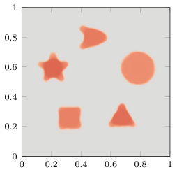


We consider inside the unknown piecewise constant medium
where denotes the characteristic function of the set , , shown in Figure 5(a). Given noisy observations , , on the boundary of , we seek to reconstruct inside .
To generate the perturbed observations , , we add white noise to the numerical solutions of (2.1) with for eight separate smoothed Gaussian point sources , each centered at a location shown in Figure 5(b). Both the observations and the scattered wave fields , needed for the inversion procedure, are discretized with a -FEM using about grid points per wavelength. To avoid any inverse crime, the observations are computed on a different, about finer mesh.
We seek our approximation of the exact medium in the -FE space for a regular, triangular mesh with vertices and elements. Since is assumed known on the boundary of , where it is constant, we choose as initial guess constant throughout ; thus, on , coincides with . To initialize the algorithm we must also choose and . To do so, we set and solve (2.6) and (2.7). Since is constant, simply reduces to the negative Laplacian times . For Step 1 of the ASI Algorithm, we use (2.17) with and .
The reconstruction of the medium at the final ASI iteration, with , is shown in Figure 5(c). Although corners appear smoothed out in the reconstruction, captures well the locations and shapes of the inclusions composing with a relative -error of .
In Figures 6(a) and 6(b), we show the misfit of the reconstructed medium and the relative error at each ASI iteration. Different markers indicate different frequencies, shown in Figure 6(c). Both the misfit and the relative error decrease until the relative error eventually levels around 0.04. In Figure 6(d), we monitor the dimension of the adaptive space at each ASI iteration. Starting at , first the dimension increases until it peaks around at iteration , and eventually decreases to about 50.
The first five basis functions of the adaptive space at the final step, , shown in Figure 7, illustrate how the adaptive basis captures the span of the first five lowest eigenfunctions in the AS decomposition.
4.2 Salt-dome model


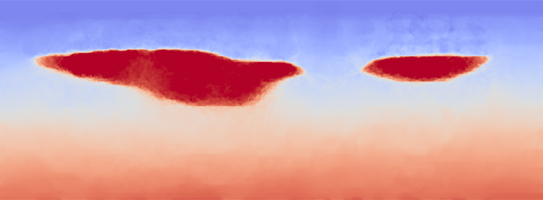
We consider a two-dimensional (Pluto 1.5) salt dome model from geosciences, generated by the “subsalt multiples attenuation and reduction technology” (SMAART) [2]. Hence, we consider (2.1a) in [km] with the squared velocity profile [km/s]2 shown in Figure 8 (top left). We impose a first order absorbing boundary condition (2.1b) on the two lateral and the lower artificial boundaries, and a homogeneous Neumann condition at the top (physical) boundary . Synthetic observations at the surface are obtained from the wave fields induced by source terms located meters beneath the top surface, each about meters apart. Again, we add white noise to the observations.
Now, we apply the ASI Algorithm to reconstruct from the surface observations. Here, we seek an approximation of the unknown medium in a -FE space with vertices and elements. The initial guess , shown in Figure 8, is generated by extending along the direction the known Eastern boundary (borehole) data to the entire computational domain. Then, starting with [Hz], the initial guess and the space spanned by the spectral basis of the negative Laplacian operator with , we solve the inverse problem (2.3) by using the ASI method while progressively increasing the frequency up to [Hz]. In Step 1 of the ASI Algorithm, we set and in (2.17).
After ASI iterations, the reconstruction , shown in Fig. 8, captures remarkably well the location, size, and inner velocities of the two salt bodies, though not originally present in the initial guess. In Fig. 9, we monitor the misfit , the dimension of the search space , and the relative -error at each ASI iteration. Both the relative -error and the misfit monotonically decrease until the error levels off at about . In Fig. 9(d), we observe that the number of basis functions of the AS space varies between and basis functions.
5 Concluding remarks
Starting from the adaptive spectral (AS) decomposition (1.1)–(1.3), we have proposed a nonlinear optimization method for the solution of inverse medium problems. Instead of a grid-based discrete representation, the unknown medium is projected at the -th iteration to a finite-dimensional affine subspace , which is updated repeatedly. The search space is constructed by combining the search space from the previous iteration with the ”background” , which satisfies (1.2), and the first eigenfunctions of a judicious linear elliptic operator . Since depends itself on the current iterate, and the orthonormal basis of eigenfunctions are updated repeatedly. Moreover, the resulting ASI (adaptive spectral inversion) algorithm, listed in Section 2.2, also adapts ”on the fly” the dimension of the search space by solving a small, quadratically constrained, quadratic minimization problem to filter basis functions while preserving important features. Hence the AS decomposition not only substantially reduces the dimension of the search space, but also removes the need for added Tikhonov-type regularization. Our numerical results for the ASI method, when applied to time-harmonic inverse scattering problems governed by the Helmholtz equation, illustrate its accuracy and efficiency even in the presence of noisy or partial boundary data. In particular, the ASI method is able to invert a two-dimensional (Pluto 1.5) salt dome model [2] from noisy surface observations with only a few hundred control variables.
Our analysis in Section 3 underpins the remarkable accuracy of the AS decomposition observed in practice. In particular, Theorem 5 provides rigorous estimates for the approximation of the background and for the eigenfunctions of , when the medium consists of piecewise constant distinct characteristic functions. Our estimates imply that and the first eigenfunctions are “almost” constant in each connected component away from interfaces. Hence for small and , the background is well approximated by , whereas the deviation from the background, (or ), may be well approximated in the span of . The analysis is valid for a wide class of medium-dependent (nonlinear) weight functions and also for different types of -regular approximations of . In particular, they also hold for standard -conforming FE approximations , where corresponds to the underlying mesh size – see Corollary 6.
The operator is related to the linearization of the total variation functional [16]. In Remark 7, we discuss similarities between Theorem 5 and the nonlinear spectral theory for the TV functional [5, 3, 1]. The comparison also raises some interesting questions we have not addressed in this work. Since our estimates are uniform in the parameters and , they suggest that a limit argument could be used for estimating the asymptotic behavior of the eigenvalues for . Interestingly, however, the present estimates are also valid for cases that are specifically excluded by the spectral theory for the TV functional [1]. More precisely, according to [1], if a set is not convex, or if its boundary is Lipschitz but not , then its characteristic function cannot be an eigenfunction for the eigenvalue (3.45) of the TV functional. Our estimates, however, then still hold true, as supported by our numerical tests in Section 3.4.
Although we have only considered scalar problems here, the AS decomposition can also be used for multiple parameters [18]. As the AS decomposition is independent of the underlying governing PDE, or any particular choice of misfit functional , it is probably also useful for other inverse problems with time-dependent or elliptic governing field equations, or possibly for different applications from image analysis.
References
- [1] G. Bellettini, V. Caselles, and M. Novaga. The total variation flow in . Journal of Differential Equations, 184(2):475 – 525, 2002.
- [2] P. Bulant. Sobolev scalar products in the construction of velocity models: Application to model Hess and to SEG/EAGE salt model. Pure and Applied Geophysics, 159(7):1487–1506, Jul 2002.
- [3] M. Burger, G. Gilboa, and M. Moeller. Nonlinear spectral analysis via one-homogeneous functionals: Overview and future prospects. Journal of Mathematical Imaging and Vision, 56(2):300–319, 2016.
- [4] G. Chavent. Nonlinear Least Squares for Inverse Problems. Springer, 2009.
- [5] D. Cremers, G. Gilboa, L. Eckardt, M. Burger, and M. Möller. Spectral decompositions using one-homogeneous functionals. CoRR, abs/1601.02912, 2016.
- [6] I. Daubechies, M. Defrise, and C. De Mol. An iterative thresholding algorithm for linear inverse problems with a sparsity constraint. Communications on Pure and Applied Mathematics, 57(11):1413–1457, 2004.
- [7] M. de Buhan and M. Darbas. Numerical resolution of an electromagnetic inverse medium problem at fixed frequency. Computers and Mathematics with Applications, 74:3111 – 3128, 2017.
- [8] M. de Buhan and M. Kray. A new approach to solve the inverse scattering problem for waves: combining the TRAC and the adaptive inversion methods. Inverse Problems, 29(8):085009, 2013.
- [9] M. de Buhan and A. Osses. Logarithmic stability in determination of a 3D viscoelastic coefficient and a numerical example. Inverse Problems, 26(9):095006, 2010.
- [10] M. C. Delfour and J.-P. Zolésio. Shapes and Geometries. Vieweg, 2 edition, 2011.
- [11] H. W. Engl, M. Hanke, and A. Neubauer. Regularization of Inverse Problems. Springer-Verlag, 2000.
- [12] L. C. Evans. Partial Differential Equations. American Mathematical Society, 2010.
- [13] L. C. Evans and R. F. Gariepy. Measure Theory and Fine Properties of Functions. CRC Press, 1992.
- [14] H. Federer. Geometric Measure Theory. Springer-Verlag, 1969.
- [15] M. Graff, M. J. Grote, F. Nataf, and F. Assous. How to solve inverse scattering problems without knowing the source term: a three-step strategy. Inverse Problems, 35:1041001, 2019.
- [16] M. Grote, M. Graff-Kray, and U. Nahum. Adaptive eigenspace method for inverse scattering problems in the frequency domain. Inverse Problems, 33:025006, 02 2017.
- [17] M. J. Grote, J. Huber, D. Kourounis, and O. Schenk. Inexact interior-point method for PDE-constrained nonlinear optimization. SIAM J. Sci. Comp., 36(3):A1251–A1276, 2014.
- [18] M. J. Grote and U. Nahum. Adaptive eigenspace for multi-parameter inverse scattering problems. Computers and Mathematics with Applications, 2019.
- [19] E. Haber, U. M. Ascher, and D. Oldenburg. On optimization techniques for solving nonlinear inverse problems. Inverse Problems, 16:1263, 2000.
- [20] F. J. Herrmann and G. Hennenfent. Non-parametric seismic data recovery with curvelet frames. Geophys. J. Int., (173):233–248, 2008.
- [21] A. Kadu, T. van Leeuwen, and W. A. Mulder. Salt reconstruction in full-waveform inversion with a parametric level-set method. IEEE Transactions on Computational Imaging, 3(2):305–315, June 2017.
- [22] B. Kaltenbacher and J. Offtermatt. A convergence analysis of regularization by discretization in preimage space. Math. Comp., 81(280):2049–2069, October 2012.
- [23] Y. Lin, A. Abubakar, and T. M. Habashy. Seismic full-waveform inversion using truncated wavelet representations. pages 1–6, 2012. SEG Annual meeting 2012, Las Vegas.
- [24] I. Loris, H. Douma, G. Nolet, I. Daubechies, and C. Regone. Nonlinear regularization techniques for seismic tomography. Journal of Computational Physics, (229):890–905, 2010.
- [25] L. Métivier, R. Brossier, J. Virieux, and S. Operto. Full waveform inversion and the truncated Newton method. SIAM J. Sci. Comput., 35(2):B401–B437, 2013.
- [26] J. Nocedal and S. J. Wright. Numerical Optimization. Springer, 2 edition, 2006.
- [27] S. Operto and J. Virieux. An overview of full-waveform inversion in exploration geophysics. Geophysics, 74:WCC1–WCC26, 11 2009.
- [28] R. G. Pratt, C. Shin, and G. J. Hicks. Gauss-Newton and full Newton methods in frequency-space seismic waveform inversion. Geophys. J. Int., 133(2):341–362, 1998.
- [29] A. Quateroni. Numerical Models for Differential Problems. Springer, 4 edition, 2008.
- [30] A. Tarantola. Inversion of seismic reflection data in the acoustic approximation. Geophysics, 49(8):1259–1266, 1984.
- [31] A. N. Tikhonov. On the stability of inverse problems. Dokl. Akad. Nauk SSSR, 39(5):195–198, 1943.