Visor: Privacy-Preserving Video Analytics as a Cloud Service
Rishabh Poddar1,2, Ganesh Ananthanarayanan2, Srinath Setty2, Stavros Volos2, Raluca Ada Popa1
1UC Berkeley 2Microsoft Research
<rishabhp,raluca>@eecs.berkeley.edu <ga,srinath,svolos>@microsoft.com
Abstract
Video-analytics-as-a-service is becoming an important offering for cloud providers. A key concern in such services is privacy of the videos being analyzed. While trusted execution environments (TEEs) are promising options for preventing the direct leakage of private video content, they remain vulnerable to side-channel attacks.
We present Visor, a system that provides confidentiality for the user’s video stream as well as the ML models in the presence of a compromised cloud platform and untrusted co-tenants. Visor executes video pipelines in a hybrid TEE that spans both the CPU and GPU. It protects the pipeline against side-channel attacks induced by data-dependent access patterns of video modules, and also addresses leakage in the CPU-GPU communication channel. Visor is up to faster than naïve oblivious solutions, and its overheads relative to a non-oblivious baseline are limited to –.
1 Introduction
Cameras are being deployed pervasively for the many applications they enable, such as traffic planning, retail experience, and enterprise security [105, 97, 104]. Videos from the cameras are streamed to the cloud, where they are processed using video analytics pipelines [115, 44, 48] composed of computer vision techniques (e.g., OpenCV [77]) and convolutional neural networks (e.g., object detector CNNs [83]); as illustrated in Figure 1. Indeed, “video-analytics-as-a-service” is becoming an important offering for cloud providers [63, 2].
Privacy of the video contents is of paramount concern in the “video analytics-as-a-service” offerings. Videos often contain sensitive information, such as users’ home interiors, people in workspaces, or license plates of cars. For example, the Kuna home monitoring service [51] transmits videos from users’ homes to the cloud, analyzes the videos, and notifies users when it detects movement in areas of interest. For user privacy, video streams must remain confidential and not be revealed to the cloud provider or other co-tenants in the cloud.
Trusted execution environments (TEEs) [61, 107] are a natural fit for privacy-preserving video analytics in the cloud. In contrast to cryptographic approaches, such as homomorphic encryption, TEEs rely on the assumption that cloud tenants also trust the hardware. The hardware provides the ability to create secure “enclaves” that are protected against privileged attackers. TEEs are more compelling than cryptographic techniques since they are orders of magnitude faster. In fact, CPU TEEs (e.g., Intel SGX [61]) lie at the heart of confidential cloud computing [39, 62]. Meanwhile, recent advancements in GPU TEEs [107, 41] enable the execution of ML models (e.g., neural networks) with strong privacy guarantees as well. CPU and GPU TEEs, thus, present an opportunity for building privacy-preserving video analytics systems.
Unfortunately, TEEs (e.g., Intel SGX) are vulnerable to a host of side-channel attacks (e.g., [109, 12, 13, 111]). For instance, in Section 2.3 we show that by observing just the memory access patterns of a widely used bounding box detection OpenCV module, an attacker can infer the exact shapes and positions of all moving objects in the video. In general, an attacker can infer crucial information about the video being processed, such as the times when there is activity, objects that appear in the video frame, all of which when combined with knowledge about the physical space being covered by the camera, can lead to serious violations of confidentiality.
We present Visor, a system for privacy-preserving video analytics services. Visor protects the confidentiality of the videos being analyzed from the service provider and other co-tenants. When tenants host their own CNN models in the cloud, it also protects the model parameters and weights. Visor protects against a powerful enclave attacker who can compromise the software stack outside the enclave, as well as observe any data-dependent accesses to network, disk, or memory via side-channels (similar to prior work [75, 82]).
Visor makes two primary contributions, combining insights from ML systems, security, computer vision, and algorithm design. First, we present a privacy-preserving framework for machine-learning-as-a-service (MLaaS), which supports CNN-based ML applications spanning both CPU and GPU resources. Our framework can potentially power applications beyond video analytics, such as medical imaging, recommendation systems, and financial forecasting. Second, we develop novel data-oblivious algorithms with provable privacy guarantees within our MLaaS framework, for commonly used vision modules. The modules are efficient and can be composed to construct many different video analytics pipelines. In designing our algorithms, we formulate a set of design principles that can be broadly applied to other vision modules as well.
1) Privacy-Preserving MLaaS Framework
Visor leverages a hybrid TEE that spans CPU and GPU resources available in the cloud. Recent work has shown that scaling video analytics pipelines requires judicious use of both CPUs and GPUs [80, 36]. Some pipeline modules can run on CPUs at the required frame rates (e.g., video decoding or vision algorithms) while others (e.g., CNNs) require GPUs, as shown in Figure 1. Thus, our solution spans both CPU and GPU TEEs, and combines them into a unified trust domain.
Visor systematically addresses access-pattern-based leakage across the components of the hybrid TEE, from video ingestion to CPU-GPU communication to CNN processing. In particular, we take the following steps:
- 1.
Visor leverages a suite of data-oblivious primitives to remove access pattern leakage from the CPU TEE. The primitives enable the development of oblivious modules with provable privacy guarantees, the access patterns of which are always independent of private data.
- 2.
Visor relies on a novel oblivious communication protocol to remove leakage from the CPU-GPU channel. As the CPU modules serve as filters, the data flow in the CPU-GPU channel (on which objects of each frame are passed to the GPU) leaks information about the contents of each frame, enabling attackers to infer the number of moving objects in a frame. At a high level, Visor pads the channel with dummy objects, leveraging the observation that our application is not constrained by the CPU-GPU bandwidth. To reduce GPU wastage, Visor intelligently minimizes running the CNN on the dummy objects.
- 3.
Visor makes CNNs running in a GPU TEE oblivious by leveraging branchless CUDA instructions to implement conditional operations (e.g., ReLU and max pooling) in a data-oblivious way.
2) Efficient Oblivious Vision Pipelines
Next, we design novel data-oblivious algorithms for vision modules that are foundational for video analytics, and implement them using the oblivious primitives provided by the framework described above. Vision algorithms are used in video analytics pipelines to extract the moving foreground objects. These algorithms (e.g., background subtraction, bounding box detection, object cropping, and tracking) run on CPUs and serve as cheap filters to discard frames instead of invoking expensive CNNs on the GPU for each frame’s objects (more in Section 2.1). The modules can be composed to construct various vision pipelines, such as medical imaging and motion tracking.
As we demonstrate in Section 8, naïve approaches for making these algorithms data-oblivious, such that their operations are independent of each pixel’s value, can slow down video pipelines by several orders of magnitude. Instead, we carefully craft oblivious vision algorithms for each module in the video analytics pipeline, including the popular VP8 video decoder [5]. Our overarching goal is to transform each algorithm into a pattern that processes each pixel identically. To apply this design pattern efficiently, we devise a set of algorithmic and systemic optimization strategies based on the properties of vision modules, as follows. First, we employ a divide-and conquer approach—i.e., we break down each algorithm into independent subroutines based on their functionality, and tailor each subroutine individually. Second, we cast sequential algorithms into a form that scans input images while performing identical operations on each pixel. Third, identical pixel operations allow us to systemically amortize the processing cost across groups of pixels in each algorithm. For each vision module, we derive the operations applied per pixel in conjunction with these design strategies. Collectively, these strategies improve performance by up to over naïve oblivious solutions. We discuss our approach in more detail in Section 5; nevertheless, we note that it can potentially help inform the design of other oblivious vision modules as well, beyond the ones we consider in Visor.
In addition, as shown by prior work, bitrate variations in encrypted network traffic can also leak information about the underlying video streams [88], beyond access pattern leakage at the cloud. To prevent this leakage, we modify the video encoder to carefully pad video streams at the source in a way that optimizes the video decoder’s latency. Visor thus provides an end-to-end solution for private video analytics.
Evaluation Highlights
We have implemented Visor on Intel SGX CPU enclaves [61] and Graviton GPU enclaves [107]. We evaluate Visor on commercial video streams of cities and datacenter premises containing sensitive data. Our evaluation shows that Visor’s vision components perform up to better than naïve oblivious solutions, and over to orders of magnitude better than a state-of-the-art general-purpose system for oblivious program execution. Against a non-oblivious baseline, Visor’s overheads are limited to – which still enables us to analyze multiple streams simultaneously in real-time on our testbed. Visor is versatile and can accommodate different combinations of vision components used in real-world applications. Thus, Visor provides an efficient solution for private video analytics.


2 Background and Motivation
2.1 Video Analytics as a Service
Figure 1 depicts the canonical pipelines for video analytics [36, 48, 115, 114, 64]. The client (e.g., a source camera) feeds the video stream to the service hosted in the cloud, which (a) decodes the video into frames, (b) extracts objects from the frames using vision algorithms, and (c) classifies the objects using a pre-trained convolutional neural network (CNN). Cameras typically offer the ability to control the resolution and frame rate at which the video streams are encoded.
Recent work demonstrates that scaling video analytics pipelines requires judicious use of both CPUs and GPUs [80, 36]. In Visor, we follow the example of Microsoft’s Rocket platform for video analytics [64, 65]—we split the pipelines by running video decoding and vision modules on the CPU, while offloading the CNN to the GPU (as shown in Figure 1). The vision modules process each frame to detect the moving “foreground” objects in the video using background subtraction [9], compute each object’s bounding box [95], and crop them from the frame for the CNN classifier. These vision modules can sustain the typical frame rates of videos even on CPUs, thereby serving as vital “filters” to reduce the expensive CNN operations on the GPU [36, 48], and are thus widely used in practical deployments. For example, CNN classification in Figure 1(a) is invoked only if moving objects are detected in a region of interest in the frame. Optionally, the moving objects are also tracked to infer directions (say, cars turning left). The CNNs can either be object classifiers (e.g., ResNet [35]) as in Figure 1(a); or object detectors (e.g., Yolo [83]) as in Figure 1(b), which take whole frames as input. The choice of pipeline modules is application dependent [44, 36] and Visor targets confidentiality for all pipeline modules, their different combinations, and vision CNNs.
While our description focuses on a multi-tenant cloud service, our ideas equally apply to multi-tenant edge compute systems, say, at cellular base stations [23]. Techniques for lightweight programmability on the cameras to reduce network traffic (e.g., using smart encoders [106] or dynamically adapting frame rates [3]) are orthogonal to Visor’s techniques.
2.2 Trusted Execution Environments
Trusted execution environments, or enclaves, protect application’s code and data from all other software in a system. Code and data loaded in an enclave—CPU and GPU TEEs—can be verified by clients using the remote attestation feature.
Intel SGX [61] enables TEEs on CPUs and enforces isolation by storing enclave code and data in a protected memory region called the Enclave Page Cache (EPC). The hardware ensures that no software outside the enclave can access EPC contents.
Graviton [107] enables TEEs on GPUs in tandem with trusted applications hosted in CPU TEEs. Graviton prevents an adversary from observing or tampering with traffic (data and commands) transferred to/from the GPU. A trusted GPU runtime (e.g., CUDA runtime) hosted in a CPU TEE attests that all code/data have been securely loaded onto the GPU.
2.3 Attacks based on Access Pattern Leakage
TEEs are vulnerable to leakage from side-channel attacks that exploit micro-architectural side-channels [13, 29, 12, 90, 67, 34, 54, 89, 20], software-based channels [111, 14], or application-specific leakage, such as network and memory accesses.

A large subset of these attacks exploit data-dependent memory access patterns (e.g., branch-prediction, cache-timing, or controlled page fault attacks). Xu et al. [111] show that by simply observing the page access patterns of image decoders, an attacker can reconstruct entire images. We ourselves analyzed the impact of access pattern leakage at cache-line granularity [29, 12, 90, 67] on the bounding box detection algorithm [95] (see Figure 1(a); §2.1). We simulated existing attacks by capturing the memory access trace during an execution of the algorithm, and then examined the trace to reverse-engineer the contents of the input frame. Since images are laid out predictably in memory, we found that the attacker is able to infer the locations of all the pixels touched during execution, and thus, the shapes and positions of all objects (as shown in Figure 2). Shapes and positions of objects are the core content of any video, and allow the attacker to infer sensitive information like times when patients are visiting private medical centers or when residents are inside a house, and even infer if the individuals are babies or on wheelchairs based on their size and shapes. In fact, conversations with customers of one of the largest public cloud providers indeed confirm that privacy of the videos is among their top-two concerns in signing up for the video analytics cloud service.
3 Threat Model and Security Guarantees
We describe the attacker’s capabilities and lay out the attacks that are in scope and out of scope for our work.
3.1 Hardware Enclaves and Side-Channels
Our trusted computing base includes: 1. the GPU package and its enclave implementation, 2. the CPU package and its enclave implementation, and 3. the video analytics pipeline implementation and GPU runtime hosted in the CPU enclave.
The design of Visor is not tied to any specific hardware enclave; instead, Visor builds on top of an abstract model of hardware enclaves where the attacker controls the server’s software stack outside the enclave (including the OS), but cannot perform any attacks to glean information from inside the processor (including processor keys). The attacker can additionally observe the contents and access patterns of all (encrypted) pages in memory, for both data and code. We assume that the attacker can observe the enclave’s memory access patterns at cache line granularity [75]. Note that our attacker model includes the cloud service provider as well as other co-tenants.
We instantiate Visor with the widely-deployed Intel SGX enclave. However, recent attacks show that SGX does not quite satisfy the abstract enclave model that Visor requires. For example, attackers may be able to distinguish intra cache line memory accesses [113, 68]. In Visor, we mitigate these attacks by disabling hyperthreading in the underlying system, disallowing attackers from observing intra-core side-channels; clients can verify that hyperthreading is disabled during remote attestation [4]. One may also employ complementary solutions for closing hyperthreading-based attacks [76, 18].
Other attacks that violate our abstract enclave model are out of scope: such as attacks based on timing analysis or power consumption [69, 96], DoS attacks [42, 32], or rollback attacks [78] (which have complementary solutions [10, 60]). Transient execution attacks (e.g., [13, 89, 17, 101, 81, 102, 103]) are also out of scope; these attacks violate the threat model of SGX and are typically patched promptly by the vendor via microcode updates. In the future, one could swap out Intel SGX in our implementation for upcoming enclaves such as MI6 [8] and Keystone [53] that address many of the above drawbacks of SGX.
Visor provides protection against any channel of attack that exploits data-dependent access patterns within our abstract enclave model, which represent a large class of known attacks on enclaves (e.g., cache attacks [29, 12, 90, 67, 34], branch prediction [54], paging-based attacks [111, 14], or memory bus snooping [52]). We note that even if co-tenancy is disabled (which comes at considerable expense), privileged software such as the OS and hypervisor can still infer access patterns (e.g., by monitoring page faults), thus still requiring data-oblivious solutions.
3.2 Video Streams and CNN Model
Each client owns its video streams, and it expects to protect its video from the cloud and co-tenants of the video analytics service. The vision algorithms are assumed to be public.
We assume that the CNN model’s architecture is public, but its weights are private and may be proprietary to either the client or the cloud service. Visor protects the weights in both scenarios within enclaves, in accordance with the threat model and guarantees from Section 3.1; however, when the weights are proprietary to the cloud service, the client may be able to learn some information about the weights by analyzing the results of the pipeline [99, 25, 26]. Such attacks are out of scope for Visor.
Finally, recent work has shown that the camera’s encrypted network traffic leaks the video’s bitrate variation to an attacker observing the network [88], which may consequently leak information about the video contents. Visor eliminates this leakage by padding the video segments at the camera, in such a way that optimizes the latency of decoding the padded stream at the cloud (§6.1).
3.3 Provable Guarantees for Data-Obliviousness
Visor provides data-obliviousness within our abstract enclave model from Section 3.1, which guarantees that the memory access patterns of enclave code does not reveal any information about sensitive data. We rely on the enclaves themselves to provide integrity, along with authenticated encryption.
We formulate the guarantees of data-obliviousness using the “simulation paradigm” [27]. First, we define a trace of observations that the attacker sees in our threat model. Then, we define the public information, i.e., information we do not attempt to hide and is known to the attacker. Using these, we argue that there exists a simulator, such that for all videos , when given only the public information (about and the video algorithms), the simulator can produce a trace that is indistinguishable from the real trace visible to an attacker who observes the access patterns during Visor’s processing of . By “indistinguishable”, we mean that no polynomial-time attacker can distinguish between the simulated trace and the real trace observed by the attacker. The fact that a simulator can produce the same observations as seen by the attacker even without knowing the private data in the video stream implies that the attacker does not learn sensitive data about the video.
In our attacker model, the trace of observations is the sequence of the addresses of memory references to code as well as data, along with the accessed data (which is encrypted). The public information is all of Visor’s algorithms, formatting and sizing information, but not the video data. For efficiency, Visor also takes as input some public parameters that represent various upper bounds on the properties of the video streams, e.g., the maximum number of objects per frame, or upper bounds on object dimensions.
In Appendix A, we provide a formal definition of data-obliviousness (Definition 1); a summary of public information for each algorithm; and proofs of security along with detailed pseudocode for each algorithm. Since Visor’s data-oblivious algorithms (Section 6 and Section 7) follow an identical sequence of memory accesses that depend only on public information and are independent of data content, our proofs are easy to verify.
4 A Privacy-Preserving MLaaS Framework
In this section, we present a privacy-preserving framework for machine-learning-as-a-service (MLaaS), that supports CNN-based ML applications spanning both CPU and GPU resources. Though Visor focuses on protecting video analytics pipelines, our framework can more broadly be used for a range of MLaaS applications such as medical imaging, recommendation systems, and financial forecasting.
Our framework comprises three key features that collectively enable data-oblivious execution of ML services. First, it protects the computation in ML pipelines using a hybrid TEE that spans both the CPU and GPU. Second, it provides a secure CPU-GPU communication channel that additionally prevents the leakage of information via traffic patterns in the channel. Third, it prevents access-pattern-based leakage on the CPU and GPU by facilitating the development of data-oblivious modules using a suite of optimized primitives.

4.1 Hybrid TEE Architecture
Figure 3 shows Visor’s architecture. Visor receives encrypted video streams from the client’s camera, which are then fed to the video processing pipeline. We refer to the architecture as a hybrid TEE as it spans both the CPU and GPU TEEs, with different modules of the video pipeline (Section 2.1) being placed across these TEEs. We follow the example of prior work that has shown that running the non-CNN modules of the pipeline on the CPU, and the CNNs on the GPU [36, 80, 64], results in efficient use of the expensive GPU resources while still keeping up with the incoming frame rate of videos.
Regardless of the placement of modules across the CPU and GPU, we note that attacks based on data access patterns can be mounted on both CPU and GPU TEEs, as explained in Section 3.1. As such, our data-oblivious algorithms and techniques are broadly applicable irrespective of the placement, though our description is based on non-CNN modules running on the CPU and the CNNs on the GPU.
CPU and GPU TEEs
We implement the CPU TEE using Intel SGX enclaves, and the GPU TEE using Graviton secure contexts [107]. The CPU TEE also runs Graviton’s trusted GPU runtime, which enables Visor to securely bootstrap the GPU TEE and establish a single trust domain across the TEEs. The GPU runtime talks to the untrusted GPU driver (running on the host outside the CPU TEE) to manage resources on the GPU via ioctl calls. In Graviton, each ioctl call is translated to a sequence of commands submitted to the command processor. Graviton ensures secure command submission (and subsequently ioctl delivery) as follows: 1. for task submission, the runtime uses authenticated encryption to protect commands from being dropped, replayed, or reordered, and 2. for resource management, the runtime validates signed summaries returned by the GPU upon completion. The GPU runtime encrypts all inter-TEE communication.
Pipeline execution
The hybrid architecture requires us to protect against attacks on the CPU TEE, GPU TEE, and the CPU-GPU channel. As Figure 3 illustrates, Visor decrypts the video stream inside the CPU TEE, and obliviously decodes out each frame (in Section 6). Visor then processes the decoded frames using oblivious vision algorithms to extract objects from each frame (in Section 7). Visor extracts the same number of objects of identical dimensions from each frame (some of which are dummies, up to an upper-bound) and feeds them into a circular buffer. This avoids leaking the actual number of objects in each frame and their sizes; the attacker can observe accesses to the buffer, even though objects are encrypted. Objects are dequeued from the buffer and sent to the GPU (Section 4.2) where they are decrypted and processed obliviously by the CNN in the GPU TEE (Section 4.3).
4.2 CPU-GPU Communication
Although the CPU-GPU channel in Figure 3 transfers encrypted objects, Visor needs to ensure that its traffic patterns are independent of the video content. Otherwise, an attacker observing the channel can infer the processing rate of objects, and hence the number (and size) of the detected objects in each frame. To address this leakage, Visor ensures that 1. the CPU TEE transfers the same number of objects to the GPU per frame, and 2. CNN inference runs at a fixed rate (or batch size) in the GPU TEE. Crucially, Visor ensures that the CNN processes as few dummy objects as possible. While our description focuses on Figure 1(a) to hide the processing rate of objects of a frame on the GPU, our techniques directly apply to the pipeline of Figure 1(b) to hide the processing rate of complete frames using dummy frames.
Since the CPU TEE already extracts a fixed number of objects per frame (say for obliviousness, we enforce an inference rate of for the CNN as well, regardless of the number of actual objects in each frame (say ). The upper bound is easy to learn for each video stream in practice. However, this leads to a wastage of GPU resources, which must now also run inference on dummy objects per frame. To limit this wastage, we develop an oblivious protocol that leads to processing as few dummy objects as possible.
Oblivious protocol
Visor runs CNN inference on objects per frame. Visor’s CPU pipeline extracts objects from each frame (extracting dummy objects if needed) and pushes them into the head of the circular buffer (Figure 3). At a fixed rate (e.g., once per frame, or every 33ms for a 30fps video), objects are dequeued from the tail of the buffer and sent to the GPU that runs inference on all objects.
We reduce the number of dummy objects processed by the GPU as follows. We sort the buffer using osort in ascending order of “priority” values (dummy objects are assigned lower priority), thus moving dummy objects to the head of the buffer and actual objects to the tail. Dequeuing from the tail of the buffer ensures that actual objects are processed first, and that dummy objects at the head of the buffer are likely overwritten before being sent to the GPU. The circular buffer’s size is set large enough to avoid overwriting actual objects.
The consumption (or inference) rate should be set relative to the actual number of objects that occur in the frames of the video stream. Too high a value of results in GPU wastage due to dummy inferences, while too low a value leads to delay in the processing of the objects in the frame (and potentially overwriting them in the circular buffer). In our experiments, we use a value of ( is the average number of objects in a frame) that leads to little delay and wastage.
Bandwidth consumption
The increase in traffic on the CPU-GPU PCIe bus (Figure 3) due to additional dummy objects for obliviousness is not an issue because the bus is not bandwidth-constrained. Even with Visor’s oblivious video pipelines, we measure the data rate to be , in contrast to the several available in PCIe interconnects.
4.3 CNN Classification on the GPU
The CNN processes identically-sized objects at a fixed rate on the GPU. The vast majority of CNN operations, such as matrix multiplications, have inherently input-independent access patterns [75, 30]. The operations that are not oblivious can be categorized as conditional assignments. For instance, the ReLU function, when given an input , replaces with 0,x; likewise, the max-pooling layer replaces each value within a square input array with its maximum value.
Oblivious implementation of the operator may use CUDA max/fmax intrinsics for integers/ floats, which get compiled to IMNMX/FMNMX instructions [74] that execute the operation branchlessly. This ensures that the code is free of data-dependent accesses, making CNN inference oblivious.
4.4 Oblivious Modules on the CPU
After providing a data-oblivious CPU-GPU channel and CNN execution on the GPU, we address the video modules (in Figure 1) that execute on the CPU. We carefully craft oblivious versions of the video modules using novel efficient algorithms (which we describe in the subsequent sections). To implement our algorithms, we use a set of oblivious primitives which we summarize below.
Oblivious primitives
We use three basic primitives, similar to prior work [82, 75, 87]. Fundamental to these primitives is the x86 CMOV instruction, which takes as input two registers—a source and a destination—and moves the source to the destination if a condition is true. Once the operands have been loaded into registers, the instructions are immune to memory-access-based pattern leakage because registers are private to the processor, making any register-to-register operations oblivious by default.
1) Oblivious assignment (oassign)
The oassign primitive is a wrapper around the CMOV instruction that conditionally assigns a value to the destination operand. This primitive can be used for performing dummy write operations by simply setting the input condition to false. We implement multiple versions of this primitive for different integer sizes. We also implement a vectorized version using SIMD instructions.
2) Oblivious sort (osort)
The osort primitive obliviously sorts an array with the help of a bitonic sorting network [6]. Given an input array of size , the network sorts the array by performing compare-and-swap operations, which can be implemented using the oassign primitive. As the network layout is fixed given the input size , execution of each network has identical memory access patterns.
3) Oblivious array access (oaccess)
The oaccess primitive accesses the -th element in an array, without leaking the value of . The simplest way of implementing oaccess is to scan the entire array. However, as discussed in our threat model (Section 3.1), hyperthreading is disabled, preventing any sharing of intra-core resources (e.g., L1 cache) with an adversary, and consequently mitigating known attacks [68, 113] that can leak access patterns at sub-cache-line granularity using shared intra-core resources. Therefore, we assume access pattern leakage at the granularity of cache lines, and it suffices for oaccess to scan the array at cache-line granularity for obliviousness, instead of per element or byte.
5 Designing Oblivious Vision Modules
Naïve approaches and generic tools for oblivious execution of vision modules can lead to prohibitive performance overheads. For instance, a naïve approach for implementing oblivious versions of CPU video analytics modules (as in Figure 1) is to simply rewrite them using the oblivious primitives outlined in Section 4.4. Such an approach: 1. eliminates all branches and replaces conditional statements with oassign operations to prevent control flow leakage via access patterns to code, 2. implements all array accesses via oaccess to prevent leakage via memory accesses to data, and 3. performs all iterations for a fixed number of times while executing dummy operations when needed. The simplicity of this approach, however, comes at the cost of high overheads: two to three orders of magnitude. Furthermore, as we show in Section 8.3, generic tools for executing programs obliviously such as Raccoon [82] and Obfuscuro [1] also have massive overheads—six to seven orders of magnitude.
Instead, we demonstrate that by carefully crafting oblivious vision modules using the primitives outlined in Section 4.4, Visor improves performance over naïve approaches by several orders of magnitude. In the remainder of this section, we present an overview of our design strategy, before diving into the detailed design of our algorithms in Section 6 and Section 7.
5.1 Design Strategy
Our overarching goal is to transform each algorithm into a pattern that processes each pixel identically, regardless of the pixel’s value. To apply this design pattern efficiently, we devise a set of algorithmic and systemic optimization strategies. These strategies are informed by the properties of vision modules, as follows.
1) Divide-and-conquer for improving performance
We break down each vision algorithm into independent subroutines based on their functionality and make each subroutine oblivious individually. Intuitively, this strategy improves performance by 1. allowing us to tailor each subroutine separately, and 2. preventing the overheads of obliviousness from getting compounded.
2) Scan-based sequential processing
Data-oblivious processing of images demands that each pixel in the image be indistinguishable from the others. This requirement presents an opportunity to revisit the design of sequential image processing algorithms. Instead of simply rewriting existing algorithms using the data-oblivious primitives from Section 4.4,
we find that recasting the algorithm into a form that scans the image, while applying the same functionality to each pixel, yields superior performance. Intuitively, this is because any non-sequential pixel access implicitly requires a scan of the image for obliviousness (e.g., using oaccess); therefore, by transforming the algorithm into a scan-based algorithm, we get rid of such non-sequential accesses.
3) Amortize cost across groups of pixels
Processing each pixel in an identical manner lends itself naturally to optimization strategies that enable batched computation over pixels—e.g., the use of data-parallel (SIMD) instructions.
In Visor, we follow the general strategy above to design oblivious versions of popular vision modules that can be composed and reused across diverse pipelines. However, our strategy can potentially help inform the design of other oblivious vision modules as well, beyond the ones we consider.
5.2 Input Parameters for Oblivious Algorithms
Our oblivious algorithms rely on a set of public input parameters that need to be provided to Visor before the deployment of the video pipelines. These parameters represent various upper bounds on the properties of the video stream, such as the maximum number of objects per frame, or the maximum size of each object.
Figure 4 summarizes the list of input parameters across all the modules of the vision pipeline.
| Component | Input parameters |
| Video decoding (Section 6) | Number of bits used to encode each (padded) row of blocks; |
| Background sub. (Section 7.1) | – |
| Bounding box detection (Section 7.2) | 1. Maximum number of objects per image; 2. Maximum number of different labels that can be assigned to pixels (an object consists of all labels that are adjacent to each other). |
| Object cropping (Section 7.3) | Upper bounds on object dimensions. |
| Object tracking (Section 7.4) | 1. An upper bound on the intermediate number of features; 2. An upper bound on the total number of features. |
| CNN Inference (Section 4.3) | – |
There are multiple ways by which these parameters may be determined. 1. The model owner may obtain these parameters simultaneously while training the model on a public dataset. 2. The client may perform offline empirical analysis of their video streams and choose a reasonable set of parameters. 3. Visor may also be augmented to compute these parameters dynamically, based on historical data (though we do not implement this). We note that providing these parameters is not strictly necessary, but meaningful parameters can significantly improve the performance of our algorithms.
6 Oblivious Video Decoding
Video encoding converts a sequence of raw images, called frames, into a compressed bitstream. Frames are of two types: keyframes and interframes. Keyframes are encoded to only exploit redundancy across pixels within the same frame. Interframes, on the other hand, use the prior frame as reference (or the most recent keyframe), and thus can exploit temporal redundancy in pixels across frames.
Encoding overview
We ground our discussion using the VP8 encoder [5], but our techniques are broadly applicable. A frame is decomposed into square arrays of pixels called blocks, and then compressed using the following steps (see Figure 5). An estimate of the block is first predicted using reference pixels (in a previous frame if interframe or the current frame if keyframe). The prediction is then subtracted from the actual block to obtain a residue. Each block in the residue is transformed into the frequency domain (e.g., using a discrete cosine transform), and its coefficients are quantized thus improving compression. Each (quantized) block is compressed into a variable-sized bitstream using a binary prefix tree and arithmetic encoding. Block prediction modes, cosine transformation, and arithmetic encoding are core to all video encoders (e.g., H264 [33], VP9 [108]) and thus our oblivious techniques carry over to all popular codecs.
The decoder reverses the steps of the encoder: 1. the incoming video bitstream is entropy decoded (Section 6.2); 2. the resulting coefficients are dequantized and inverse transformed to obtain the residual block (Section 6.3); and 3. previously decoded pixels are used as reference to obtain a prediction block, which are then added to the residue (Section 6.4).
6.1 Video Encoder Padding
While the video stream is in transit, the bitrate variation of each frame is visible to an attacker observing the network even if the traffic is TLS-encrypted. This variability can be exploited for fingerprinting video streams [88] and understanding its content. Overcoming this leakage requires changes to the video encoder to “pad” each frame with dummy bits to an upper bound before sending the stream to Visor.
We modify the video encoder to pad the encoded video streams. However, instead of applying padding at the level of frames, we pad each individual row of blocks within the frames. Compared to frame-level padding, padding individual rows of blocks significantly improves latency of oblivious decoding, but at the cost of an increase in network bandwidth.
Padding the frames of the video stream, however, negates the benefit of using interframes during encoding of the raw video stream, which are typically much smaller than keyframes. We therefore configure the encoder to encode all raw video frames into keyframes, which eliminates the added complexity of dealing with interframes, and consequently simplifies the oblivious decoding procedure.
We note that it may not always be possible to modify legacy cameras to incorporate padding. In such cases, potential solutions include the deployment of a lightweight edge-compute device that pads input camera feeds before streaming them to the cloud. For completeness, we also discuss the impact of the lack of padding in Appendix B, along with the accompanying security-performance tradeoff.
6.2 Bitstream Decoding
The bitstream decoder reconstructs blocks with the help of a prefix tree. At each node in the tree it decodes a single bit from the compressed bitstream via arithmetic decoding, and traverses the tree based on the value of the bit. While decoding the bit, the decoder first checks whether any more bits can be decoded at the current bitstream position, and if not, it advances the bitstream pointer by two bytes. Once it reaches a leaf node, it outputs a coefficient based on the position of the leaf, and assigns the coefficient to the current pixel in the block. This continues for all the coefficients in the frame.
Requirements for obliviousness
The above algorithm leaks information about the compressed bitstream. First, the traversal of the tree leaks the value of the parsed coefficient. For obliviousness, we need to ensure that during traversal, the identity of the current node being processed remains secret. Second, not every position in the bitstream encodes the same number of coefficients, and the bitstream pointer advances variably during decoding. Hence, this leaks the number of coefficients that are encoded per two-byte chunk (which may convey their values). We design a solution that decouples the parsing of coefficients, i.e., prefix tree traversal (Section 6.2.1), from the assignment of the parsed coefficients to pixels (Section 6.2.2).
6.2.1 Oblivious prefix tree traversal
A simple way to make tree traversal oblivious is to represent the prefix tree as an array. We can then obliviously fetch any node in the tree using oaccess (Section 4.4). Though this hides the identity of the fetched node, we need to also ensure that processing of the nodes does not leak their identity.
In particular, we need to ensure that nodes are indistinguishable from each other by performing an identical set of operations at each node. Unfortunately, this requirement is complicated by the following facts. (1) Only leaf nodes in the tree produce outputs (i.e., the parsed coefficients) and not the intermediate nodes. (2) We do not know beforehand which nodes in the tree will cause the bitstream pointer to be advanced; at the same time, we need to ensure that the pointer is advanced predictably and independent of the bitstream. To solve these problems, we take the following steps.
- 1)
We modify each node to output a coefficient regardless of whether it is a leaf state or not. Leaves output the parsed coefficient, while other states output a dummy value.
- 2)
We introduce a dummy node into the prefix tree. While traversing the tree, if no more bits can be decoded at the current bitstream position, we transition to the dummy node and perform a bounded number of dummy decodes.
These modifications ensure that while traversing the prefix tree, all that an attacker sees is that at some node in the tree, a single bit was decoded and a single value was outputted.
Note that in this phase, we do not assign coefficients to pixels, and instead collect them in a list. If we were to assign coefficients to pixels in this phase, then the decoder would need to obliviously scan the entire frame (using oaccess) at every node in the tree, in order to hide the pixel’s identity. Instead, by decoupling parsing from assignment, we are able to perform the assignment obliviously using a super-linear number of accesses (instead of quadratic), as we explain next.
6.2.2 Oblivious coefficient assignment
At the end of Section 6.2.1, we have a list of actual and dummy coefficients. The key idea is that if we can obliviously sort this set of values using osort such that all the actual coefficients are contiguously ordered while all dummies are pushed to the front, then we can simply read the coefficients off the end of the list sequentially and assign them to pixels one by one.
To enable such a sort, we modify the prefix tree traversal to additionally output a tuple per coefficient; flag is 0 for dummies and 1 otherwise; index is an increasing counter as per the pixel’s index. Then, the desired sort can be achieved by sorting the list based on the value of the tuple.
As the complexity of oblivious sort is super-linear in the number of elements being sorted, an important optimization is to decode and assign coefficients to pixels at the granularity of rows of blocks rather than frames. While the number of bits per row of blocks may be observed, the algorithm’s obliviousness is not affected as each row of blocks in the video stream is padded to an upper bound (Section 6.1); had we applied frame-level padding, this optimization would have revealed the number of bits per row of blocks. In Section 8.1.1, we show that this technique improves oblivious decoding latency by .
6.3 Dequantization and Inverse Transformation
The next step in the decoding process is to 1. dequantize the coefficients decoded from the bitstream, followed by 2. inverse transformation to obtain the residual blocks. Dequantization just multiplies each coefficient by a quantization factor. The inverse transformation also performs a set of identical arithmetic operations irrespective of the coefficient values.
6.4 Block Prediction
Prediction is the final stage in decoding. The residual block obtained after Section 6.3 is added to a predicted block, obtained using a previously constructed block as reference, to obtain the raw pixel values. In keyframes, each block is intra-predicted—i.e., it uses a block in the same frame as referenced. We do not discuss interframes because as described in Section 6.1, the padded input video streams in Visor only contain keyframes.
Intra-predicted blocks are computed using one of several modes. A mode to encode a block refers to a combination of pixels on its top row and left column used as reference. Obliviousness requires that the prediction mode remains private. Otherwise, an attacker can identify the pixels that are most similar to each other, thus revealing details about the frame.
We make intra-prediction oblivious by evaluating all possible predictions for the pixel and storing them in an array, indexing each prediction by its mode. Then, we use oaccess to obliviously select the correct prediction from the array.
7 Oblivious Image Processing
After obliviously decoding frames in Section 6, the next step as shown in Figure 1 is to develop data-oblivious techniques for background subtraction (Section 7.1), bounding box detection (Section 7.2), object cropping (Section 7.3), and tracking (Section 7.4). We present the key ideas here; detailed pseudocode and proofs of obliviousness are available in Section A.2. Note that Section 7.1 and Section 7.4 modify popular algorithms to make them oblivious, while Section 7.2 and Section 7.3 propose new oblivious algorithms.
7.1 Background Subtraction
The goal of background subtraction is to detect moving objects in a video. Specifically, it dynamically learns stationary pixels that belong to the video’s background, and then subtracts them from each frame, thus producing a binary image with black background pixels and white foreground pixels.
Zivkovic et al. proposed a mechanism [116, 117] that is widely used in practical deployments, that models each pixel as a mixture of Gaussians [9]. The number of Gaussian components differs across pixels depending on their value (but is no more than , a pre-defined constant). As more data arrives (with new frames), the algorithm updates each Gaussian component along with their weights (), and adds new components if necessary.
To determine if a pixel belongs to the background or not, the algorithm uses the Gaussian components with the largest weights and outputs true if is larger than a threshold:
where and are parameters of the Gaussian components, and is the weight of the -th Gaussian component.
This algorithm is not oblivious because it maintains a different number of Gaussian components per pixel, and thus performs different steps while updating the mixture model per pixel. These differences are visible via access patterns, and these leakages reveal to an attacker how complex a pixel is in relation to others—i.e., whether a pixel’s value stays stable over time or changes frequently. This enables the attacker to identify the positions of moving objects in the video.
For obliviousness, we need to perform an identical set of operations per pixel (regardless of their value); we thus always maintain Gaussian components for each pixel, of which are dummy components and assigned a weight . When newer frames arrive, we use oassign operations to make all the updates to the mixture model, making dummy operations for the dummy components. Similarly, to select the largest components by weight, we use the osort primitive.
7.2 Bounding Box Detection
The output from §7.1 is a binary image with black background pixels where the foreground objects are white blobs (Figure 6(a)). To find these objects, it suffices to find the edge contours of all blobs. These are used to compute the bounding rectangular box of each object. A standard approach for finding the contours in a binary image is the border following algorithm of Suzuki and Abe [95]. As the name suggests, the algorithm works by scanning the image until it locates an edge pixel, and then follows the edge around a blob. As Figure 2 in Section 2.3 illustrated, the memory access patterns of this algorithm leak the details of all the objects in the frame.
A naïve way to make this algorithm oblivious is to implement each pixel access using the oaccess primitive (along with other minor modifications). However, we measure that this approach slows down the algorithm by over .
We devise a two-pass oblivious algorithm for computing bounding boxes by adapting the classical technique of connected component labeling (CCL) [85]. The algorithm’s main steps are illustrated in Figure 6(a) (whose original binary image contains two blobs). In the first pass, it scans the image and assigns each pixel a temporary label if it is “connected” to other pixels. In the second pass, it merges labels that are part of a single object. Even though CCL on its own is less efficient for detecting blobs than border following, it is far more amenable to being adapted for obliviousness.
We make this algorithm oblivious as follows. First, we perform identical operations regardless of whether the current pixel is connected to other pixels. Second, for efficiency, we restrict the maximum number of temporary labels (in the first pass) to a parameter provided as input to Visor (per Section 5.2, Figure 4). Note that the value of the parameter may be much lower than the worst case upper bound (which is the total number of pixels), and thus is more efficient.
Enhancement via parallelization
We observe that the oblivious algorithm can be parallelized using a divide-and-conquer approach. We divide the frame into horizontal stripes ( in Figure 6(b)) and process each stripe in parallel (). For objects that span stripe boundaries, each stripe outputs only a partial bounding box containing the pixels within the stripe. We combine the partial boxes by re-applying the oblivious CCL algorithm to the boundaries of adjacent stripes (). Given two adjacent stripes and one below the other, we compare each pixel in the top row of with its neighbors in the bottom row of , and merge their labels as required.
7.3 Object Cropping
The next step after detecting bounding boxes of objects is to crop them out of the frame to be sent for CNN classification (Figure 1(a)). Visor needs to ensure that the cropping of objects does not leak 1. their positions, or 2. their dimensions.
7.3.1 Hiding object positions
A naïve way of obliviously cropping an object of size is to slide a window (of size ) horizontally in raster order, and copy the window’s pixels if it aligns with the object’s bounding box. Otherwise, perform a dummy copy. This, however, leads to a slow down of , with the major reason being redundant copies: while sliding the window forward by one pixel results in a new position in the frame, a majority of the pixels copied are the same as in the previous position.
We get rid of this redundancy by decoupling the algorithm into multiple passes—one pass along each dimension of the image—such that each pass performs only a subset of the work. As Figure 7(a) shows, the first phase extracts the horizontal strip containing the object; the second phase extracts the object from the horizontal strip.
Instead of sliding a window (of size ) across the frame (of size ), we use a horizontal strip of that has width equal to that of the frame, and height equal to that of the object. We slide the strip vertically down the frame row by row. If the top and bottom edges of the strip are aligned with the object, we copy all pixels covered by the strip into the buffer; otherwise, we perform dummy copies.
We allocate a window of size equal to the object’s size and then slide it column by column across the extracted strip in . If the left and right edges of the window are aligned with the object’s bounding box, we copy the window’s pixels into the buffer; if not, we perform dummy copies.
Algorithm 4 in Section A.2 provides the detailed steps.
7.3.2 Hiding object dimensions
The algorithm in Section 7.3.1 leaks the dimensions of the objects. To hide object dimensions, Visor takes as input parameters and representing upper bounds on object dimensions (as described in Section 5.2, Figure 4), and instead of cropping out the exact object, we obliviously crop out a larger image of size that subsumes the object. While the object sizes vary depending on their position in the frame (e.g., near or far from the camera), the maximum values ( and ) can be learned from profiling just a few sample minutes of the video, and they tend to remain unchanged in our datasets.
This larger image now contains extraneous pixels surrounding the object, which might lead to errors during the CNN’s object classification. We remove the extraneous pixels surrounding the object by obliviously scaling it up to fill the buffer. Note that all objects we send to the CNN across the CPU-GPU channel are of size (Section 4.2), and recall from Section 4.1 that we extract the same number of objects from each frame (by padding dummy objects, if needed).
We develop an oblivious routine for scaling up using bilinear interpolation [40].
Bilinear interpolation computes the value of a pixel in the scaled up image using a linear combination of a array of pixels from the original image (see Figure 7(b)). We once again use decoupling of the algorithm into two passes to improve its efficiency (Figure 7(c)) by scaling up along a single dimension per pass.
Cache locality
Since the second pass of our (decoupled bilinear interpolation) algorithm performs column-wise interpolations, each pixel access during the interpolation touches a different cache line. To exploit cache locality, we transpose the image before the second pass, and make the second pass to also perform row-wise interpolations (as in the first pass). This results in another order of magnitude speedup (Section 8.1.4).
7.4 Object Tracking
Object tracking consists of two main steps: feature detection in each frame and feature matching across frames.
Feature detection
SIFT [57, 58] is a popular algorithm for extracting features for keypoints, i.e., pixels that are the most “valuable” in the frame. In a nutshell, it generates candidate keypoints, where each candidate is a local maxima/minima; the candidates are then filtered to get the legitimate keypoints.
Based on the access patterns of the SIFT algorithm, an attacker can infer the locations of all the keypoints in the image, which in turn, can reveal the location of all object “corners” in the image. A naïve way of making the algorithm oblivious is to treat each pixel as a keypoint, performing all the above operations for each. However, the SIFT algorithm’s performance depends critically on its ability to filter out a small set of good keypoints from the frame.
To be oblivious and efficient, Visor takes as input two parameters and (per Figure 4). The parameter represents an upper bound on the number of candidate keypoints, and on the number of legitimate keypoints. These parameters, coupled with oassign and osort, allow for efficient and oblivious identification of keypoints. Finally, computing the feature descriptors for each keypoint requires accessing the pixels around it. For this, we use oblivious extraction (Section 7.3). Section A.2’s Algorithm 6 has the pseudocode.
Feature matching
The next step after detecting features is to match them across images. Feature matching computes a distance metric between two sets of features, and identifies features that are “nearest” to each other in the two sets. In Visor, we simply perform brute-force matching of the two sets, using oassign operations to select the closest features.
8 Evaluation
Implementation
We implement our oblivious video decoder atop FFmpeg’s VP8 decoder [24] and oblivious vision algorithms atop OpenCV 3.2.0 [77]. We use Caffe [43] for running CNNs. We encrypt data channels using AES-GCM. We implement the oblivious primitives of Section 4.4 using inline assembly code (as in [75, 82, 87]), and manually verified the binary to ensure that compiler optimizations do not undo our intent; one can also use tools such as Vale [7] to do the same.
Testbed
We evaluate Visor on Intel i7-8700K with 6 cores running at , and an NVIDIA GTX 780 GPU with 2304 CUDA cores running at . We disable hyperthreading for experiments with Visor (per Section 3), but retain hyperthreading in the insecure baseline. Disabling hyperthreading for security does not sacrifice the performance of Visor (due to its heavy utilization of vector units) unlike the baseline system that favors hyperthreading; see Appendix C for more details. The server runs Linux v4.11; supports AVX2 and SGX-v1 instruction sets; and has of memory, with of enclave memory. The GPU has of memory.
Datasets
We use four real-world video streams (obtained with permission) in our experiments: streams 1 and 4 are from traffic cameras in the city of Bellevue (resolution ) while streams 2 and 3 are sourced from cameras surveilling commercial datacenters (resolution ). All these videos are privacy-sensitive as they involve government regulations or business sensitivity. For experiments that evaluate the cost of obliviousness across different resolutions and bitrates, we re-encode the videos accordingly. A recent body of work [48, 44, 115] has found that the accuracy of object detection in video streams is not affected if the resolution is decreased (while consuming significantly lesser resources), and 720p videos suffice. We therefore chose to use streams closer to 720p in resolution because we believe they would be a more accurate representation of real performance.
Evaluation highlights
We summarize the key takeaways of our evaluation.
- 1)
Visor’s optimized oblivious algorithms (Section 6, Section 7) are up to faster than naïve competing solutions. (Section 8.1)
- 2)
End-to-end overhead of obliviousness for real-world video pipelines with state-of-the-art CNNs are limited to – over a non-oblivious baseline. (Section 8.2)
- 3)
Visor is generic and can accommodate multiple pipelines (Section 2.1; Figure 1) that combine the different vision processing algorithms and CNNs. (Section 8.2)
- 4)
Visor’s performance is over 6 to 7 orders of magnitude better than a state-of-the-art general-purpose system for oblivious program execution. (Section 8.3)
Overall, Visor’s use of properties of the video streams has no impact on the accuracy of the analytics outputs.
8.1 Performance of Oblivious Components
We begin by studying the performance of Visor’s oblivious modules: we quantify the raw overhead of our algorithms (without enclaves) over non-oblivious baselines; we also measure the improvements over naïve oblivious solutions.
8.1.1 Oblivious video decoding
Decoding of the compressed bitstream dominates decoding latency, consuming up to of the total latency. Further, this stage is dominated by the oblivious assignment subroutine which sorts coefficients into the correct pixel positions using osort, consuming up to of the decoding latency. Since the complexity of oblivious sort is super-linear in the number of elements being sorted, our technique for decoding at the granularity of rows of blocks rather than frames significantly improves the latency of oblivious decoding.
Overheads
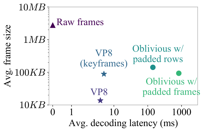
Figure 10 shows the bandwidth usage and decoding latency for different oblivious decoding strategies (i.e., decoding at the level of frames, or at the level of row of blocks) for a video stream of resolution . We also include two reference points: non-encoded frames and VP8 encoding. The baseline latency of decoding VP8 encoded frames is –. Non-encoded raw frames incur no decoding latency but result in frames that are three orders of magnitude larger than the VP8 average frame size (10s of ) at a bitrate of .
Frame-level oblivious decoding introduces high latency (), which is two orders of magnitude higher than non-oblivious counterparts. Furthermore, padding each frame to prevent leakage of the frame’s bitrate increases the average frame size to . On the contrary, oblivious decoding at the level of rows of blocks delivers , which is lower than frame-level decoding. However, this comes with a modest increase in network bandwidth as the encoder needs to pad each row of blocks individually, rather than a frame. In particular, the frame size increases from to .
Apart from the granularity of decoding, the latency of the oblivious sort is also governed by: 1. the frame’s resolution, and 2. the bitrate. The higher the frame’s resolution / bitrate, the more coefficients there are to be sorted. Figure 10 plots oblivious decoding latency at the granularity of rows of blocks across video streams with different resolutions and bitrates. The figure shows that lower resolution/bitrates introduce lower decoding overheads. In many cases, lower image qualities are adequate for video analytics as it does not impact the accuracy of the object classification [44].

8.1.2 Background subtraction
We set the maximum number of Gaussian components per pixel , following prior work [116, 117]. Our changes for obliviousness enable us to make use of SIMD instructions for updating the Gaussian components in parallel. This is because we now maintain the same number of components per pixel, and update operations for each component are identical.
Figure 10 plots the overhead of obliviousness on background subtraction across different resolutions. The SIMD implementation increases the latency of the routine only by over the baseline non-oblivious routine. As the routine processes each pixel in the frame independent of the rest, its latency increases linearly with the total number of pixels.
8.1.3 Bounding box detection
For non-oblivious bounding box detection, we use the border-following algorithm of Suzuki and Abe [95] (per Section 7.2); this algorithm is efficient, running in sub-millisecond latencies.
The performance of our oblivious bounding box detection algorithm is governed by two parameters: 1. the number of stripes used in the divide-and-conquer approach, which controls the degree of parallelism, and 2. an upper bound on the maximum number of labels possible per stripe, which determines the size of the algorithm’s data structures.
Figure 12 plots for streams of different frame resolutions while varying the number of stripes into which each frame is divided. As expected, as the number of stripes increases, the value of required per stripe decreases. Similarly, lower resolution frames require smaller values of .
Figure 12 plots the latency of detecting all bounding boxes in a frame based on the value of the parameter , ranging from a few milliseconds to hundreds of milliseconds. For a given resolution, the latency decreases as the number of stripes increase, due to two reasons: 1. increased parallelism, and 2. smaller sizes of required per stripe. Overall, the divide-and-conquer approach reduces latency by an order of magnitude down to a handful of milliseconds.
8.1.4 Object cropping
We first evaluate oblivious object cropping while leaking object sizes. We include three variants: the naïve approach; the two-phase approach; and a further optimization that advances the sliding window forward multiple rows/columns at a time. Figure 15 plots the cost of cropping variable-sized objects from a frame, showing that the proposed refinements reduce latency by three orders of magnitude .
Figure 15 plots the latency of obliviously resizing the target ROI within a cropped image to hide the object’s size. While the latency of naïve bilinear interpolation is high (10s of milliseconds) for large objects, the optimized two-pass approach (that exploits cache locality by transposing the image before the second pass; Section 7.3.2) reduces latency by two orders of magnitude down to one millisecond for large objects.
8.1.5 Object tracking
Figure 15 plots the latency of object tracking with and without obliviousness. We examine our sample streams at various resolutions to determine upper bounds on the maximum number of features in frames. As the resolution increases, the overhead of obliviousness increases as well because our algorithm involves an oblivious sort of the intermediate set of detected features, the cost of which is superlinear in the size of the set. Overall, the overhead is .
8.1.6 CNN classification on GPU
Buffer
Figure 18 benchmarks the sorting cost as a function of the object size and the buffer size. For buffer sizes smaller than 50, the sorting cost remains under .
Inference
We measure the performance of CNN object classification on the GPU. As discussed in Section 4.3, oblivious inference comes free of cost. Figure 18 lists the throughput of different CNN models using the proprietary NVIDIA driver, with CUDA version 9.2. Each model takes as input a batch of 10 objects of size . Further, since GPU memory is limited to , we also list the maximum number of concurrent models that can run on our testbed. As we show in Section 8.2, the latter has a direct bearing on the number of video analytics pipelines that can be concurrently served.
| CNN | Batches/s | Max no. of models |
| AlexNet | 40.3 | 7 |
| ResNet-18 | 18.4 | 4 |
| ResNet-50 | 8.2 | 1 |
| VGG-16 | 5.4 | 1 |
| VGG-19 | 4.4 | 1 |
| Yolo | 3.9 | 1 |
8.2 System Performance
We now evaluate the end-to-end performance of the video analytics pipeline using four real video streams. We present the overheads of running Visor’s data-oblivious techniques and hosting the pipeline in a hybrid enclave. We evaluate the two example pipelines in Figure 1: pipeline 1 uses an object classifier CNN; pipeline 2 uses an object detector CNN (Yolo), and performs object tracking on the CPU.
Pipeline 1 configuration. We run inference on objects that are larger than 1% of the frame size as smaller detected objects do not represent any meaningful value. Across our videos, the number of such objects per frame is small—no frame has more than 5 objects, and 97-99% of frames have less than 2 to 3 objects. Therefore, we configure: 1. Visor’s object detection stage to conservatively output 5 objects per frame (including dummies) into the buffer, 2. the consumption rate of Visor’s CNN module to 2 or 3 objects per frame (depending on the stream), and 3. the buffer size to 50, which suffices to prevent non-dummy objects from being overwritten.
Pipeline 2 configuration. The Yolo object detection CNN ingests entire frames, instead of individual objects. In the baseline, we filter frames that don’t contain any objects using background subtraction. However, we forego this filtering in the oblivious version since most frames contain foreground objects in our sample streams. Additionally, Yolo expects the frames to be of resolution . So we resize the input video streams to be of the same resolution.
Cost of obliviousness
Figures 18 and 21 plot the overhead of Visor on the CPU-side components of pipelines 1 and 2, while varying the number of concurrent pipelines. Visor reduces peak CPU throughput by – across the two pipelines, compared to the non-oblivious baseline. However, the throughput of the system ultimately depends on the number of models that can fit in GPU memory.
Figure 21 plots Visor’s end-to-end performance for both pipelines, across all four sample video streams. In the presence of CNN inference, Visor’s overheads depend on the model complexity. Pipelines that utilize light models, such as AlexNet and ResNet-18, are bottlenecked by the CPU. In such cases, the overhead is determined by the cost of obliviousness incurred by the CPU components. With heavier models such as ResNet-50 and VGG, the performance bottleneck shifts to the GPU. In this case, the overhead of Visor is governed by the amount of dummy objects processed by the GPU (as described in Section 4.2). Overall, the cost of obliviousness remains in the range of – across video streams for the first pipeline. In the second pipeline, the overhead is . The GPU can fit only a single Yolo model. The overall performance, however, is bottlenecked at the CPU because the object tracking routine is relatively expensive.
Cost of enclaves
We measure the cost of running the pipelines in CPU/GPU enclaves by replacing the NVIDIA stack with Graviton’s stack, which comprises open-source CUDA runtime (Gdev [50]) and GPU driver (Nouveau [73]).
Figure 21 compares Visor against a non-oblivious baseline when both systems are hosted in CPU/GPU enclaves. As SGX’s EPC size is limited to , workloads with large memory footprints incur high overhead. For pipeline 1, and for large frame resolutions, the latency of background subtraction increases from to due to its working set size being . In Visor, the pipeline’s net latency increases by (as SGX overheads mask some of Visor’s overheads) while increasing the memory footprint to . When the pipeline operates on lower frame resolutions, such that its memory footprint fits within current EPC, the latency of the non-oblivious baseline tracks the latency of the insecure baseline (a few milliseconds); the additional overhead of obliviousness is .
For pipeline 2, the limited EPC increases the latency of object tracking from to . With Visor’s obliviousness, the net latency increases by .
8.3 Comparison against Prior Work
We conclude our evaluation by comparing Visor against Obfuscuro [1], a state-of-the-art general-purpose system for oblivious program execution.
The current implementation of Obfuscuro supports a limited set of instructions, and hence cannot run the entire video analytics pipeline. On this note, we ported the OpenCV object cropping module to Obfuscuro, which requires only simple assignment operations. Cropping objects of size and (from a image) takes hours and minutes in Obfuscuro respectively, versus and in Visor; making Visor faster by over to orders of magnitude. We note, however, that Obfuscuro targets stronger guarantees than Visor as it also aims to obfuscate the programs; hence, it is not a strictly apples-to-apples comparison. Nonetheless, the large gap in performance is hard to bridge, and our experiments demonstrate the benefit of Visor’s customized solutions.
Other tools for automatically synthesizing or executing oblivious programs are either closed-source [82, 110], require special hardware [72, 55, 59], or require custom language support [16]. However, we note that the authors of Raccoon [82] (which provides similar levels of security as Visor) report up to overhead on toy programs; the overhead would arguably be higher for complex programs like video analytics.
9 Discussion
Attacks on upper bounds
For efficiency, Visor extracts a fixed number of objects per frame based on a user-specified upper bound. However, this leaves Visor open to adversarial inputs: an attacker who knows this upper bound can attempt to confuse the analytics pipeline by operating many objects in the frame at the same time.
To mitigate such attacks, we suggest two potential strategies: 1. For frames containing objects (as detected in Section 7.2), process those frames off the critical path using worst-case bounds (e.g., total number of pixels). While this approach leaks which specific frames contain objects, the leakage may be acceptable considering these frames are suspicious. 2. Filter objects based on their properties like object size or object location: e.g., for a traffic feed, only select objects at the center of the traffic intersection. This limits the number of valid objects possible per frame, raising the bar for mounting such attacks. One can also apply richer filters on the pipeline results and reprocess frames with suspicious content.
Oblivious-by-design encoding
Instead of designing oblivious versions of existing codecs, it may be possible to construct an oblivious-by-design coding scheme that is 1. potentially simpler, and 2. performs better than Visor’s oblivious decoding. This alternate design point is an interesting direction for future work. We note, however, that any such codec would need to produce a perfectly constant bitrate (CBR) per frame to prevent bitrate leakage over the network. While CBR codecs have been explored in the video literature, they are inferior to variable bitrate schemes (VBR) such as VP8 because they are lossier. In other words, an oblivious CBR scheme would consume greater bandwidth than VP8 to match its video quality (and therefore, VP8 with padding), though it may indeed be simpler. In Visor, we optimize for quality.
10 Related Work
To the best of our knowledge, Visor is the first system for the secure execution of vision pipelines. We discuss prior work related to various aspects of Visor.
Video processing systems
A wide range of optimizations have been proposed to improve the efficiency of video analytic pipelines [36, 48, 44, 115]. These systems offer different design points for enabling trade-offs between performance and accuracy. Their techniques are complementary to Visor which can benefit from their performance efficiency.
Data-oblivious techniques
Eppstein et al. [22] develop data-oblivious algorithms for geometric computations. Ohrimenko et al. [75] propose data-oblivious machine learning algorithms running inside CPU TEEs. These works are similar in spirit to Visor, but are not applicable to our setting.
Oblivious RAM [28] is a general-purpose cryptographic solution for eliminating access-pattern leakage. While recent advancements have reduced its computational overhead [94], it still remains several orders of magnitude more expensive than customized solutions. Oblix [66] and Zerotrace [87] enable ORAM support for applications running within hardware enclaves, but have similar limitations.
Various systems [82, 55, 1, 93, 72, 59, 110, 16] also offer generic solutions for hiding access patterns at different levels, with the help of ORAM, specialized hardware, or compiler-based techniques. Generic solutions, however, are less efficient than customized solutions (such as Visor) which can exploit algorithmic patterns for greater efficiency.
Side-channel defenses for TEEs
Visor provides systemic protection against attacks that exploit access pattern leakage in enclaves. Systems for data-oblivious execution (such as Obfuscuro [1] and Raccoon [82]) provide similar levels of security for general-purpose workloads, while Visor is tailored to vision pipelines.
In contrast, a variety of defenses have also been proposed to detect [19] or mitigate specific classes of access-pattern leakage. For example, Cloak [31], Varys [76], and Hyperrace [18] target cache-based attacks; while T-SGX [91] and Shinde et al. [92] propose defenses for paging-based attacks. DR.SGX [11] mitigates access pattern leakage by frequently re-randomizing data locations, but can leak information if the enclave program makes predictable memory accesses.
Telekine [37] mitigates side-channels in GPU TEEs induced by CPU-GPU communication patterns, similar to Visor’s oblivious CPU-GPU communication protocol (though the latter is specific to Visor’s use case).
Secure inference
Several recent works propose cryptographic solutions for CNN inference [47, 56, 21, 86, 84] relying on homomorphic encryption and/or secure multi-party computation [112]. While cryptographic approaches avoid the pitfalls of TEE-based CNN inference, the latter remains faster by orders of magnitude [98, 38].
11 Conclusion
We presented Visor, a system that enables privacy-preserving video analytics services. Visor uses a hybrid TEE architecture that spans both the CPU and the GPU, as well as novel data-oblivious vision algorithms. Visor provides strong confidentiality and integrity guarantees, for video streams and models, in the presence of privileged attackers and malicious co-tenants. Our implementation of Visor shows limited performance overhead for the provided level of security.
Acknowledgments
We are grateful to Chia-Che Tsai for helping us instrument the Graphene LibOS. We thank our shepherd, Kaveh Razavi, and the anonymous reviewers for their insightful comments. We also thank Stefan Saroiu, Yuanchao Shu, and members of the RISELab at UC Berkeley for helpful feedback on the paper. This work was supported in part by the NSF CISE Expeditions Award CCF-1730628, and gifts from the Sloan Foundation, Bakar Program, Alibaba, Amazon Web Services, Ant Financial, Capital One, Ericsson, Facebook, Futurewei, Google, Intel, Microsoft, Nvidia, Scotiabank, Splunk, and VMware.
References
- [1] A. Ahmad, B. Joe, Y. Xiao, Y. Zhang, I. Shin, and B. Lee. Obfuscuro: A Commodity Obfuscation Engine on Intel SGX. In NDSS, 2019.
- [2] Amazon Rekognition. https://aws.amazon.com/rekognition/.
- [3] G. Ananthanarayanan, V. Bahl, P. Bodík, K. Chintalapudi, M. Philipose, L. R. Sivalingam, and S. Sinha. Real-time Video Analytics – the killer app for edge computing. IEEE Computer, 2017.
- [4] Attestation Service for Intel SGX. https://api.trustedservices.intel.com/documents/sgx-attestation-api-spec.pdf.
- [5] J. Bankoski, P. Wilkins, and Y. Xu. Technical overview of VP8, an open source video codec for the web. In ICME, 2011.
- [6] K. E. Batcher. Sorting Networks and Their Applications. In Proceedings of the Spring Joint Computer Conference, 1968.
- [7] B. Bond, C. Hawblitzel, M. Kapritsos, K. R. M. Leino, J. R. Lorch, B. Parno, A. Rane, S. Setty, and L. Thompson. Vale: Verifying High-Performance Cryptographic Assembly Code. In USENIX Security, 2017.
- [8] T. Bourgeat, I. Lebedev, A. Wright, S. Zhang, Arvind, and S. Devadas. MI6: Secure Enclaves in a Speculative Out-of-Order Processor. In MICRO, 2019.
- [9] T. Bouwmans, F. E. Baf, and B. Vachon. Background Modeling using Mixture of Gaussians for Foreground Detection – A Survey. Recent Patents on Computer Science, 2008.
- [10] M. Brandenburger, C. Cachin, M. Lorenz, and R. Kapitza. Rollback and Forking Detection for Trusted Execution Environments using Lightweight Collective Memory. In DSN, 2017.
- [11] F. Brasser, S. Capkun, A. Dmitrienko, T. Frassetto, K. Kostiainen, and A.-R. Sadeghi. DR.SGX: Automated and Adjustable Side-Channel Protection for SGX Using Data Location Randomization. In ACSAC, 2019.
- [12] F. Brasser, U. Müller, A. Dmitrienko, K. Kostiainen, S. Capkun, and A. Sadeghi. Software Grand Exposure: SGX Cache Attacks Are Practical. In WOOT, 2017.
- [13] J. V. Bulck, M. Minkin, O. Weisse, D. Genkin, B. Kasikci, F. Piessens, M. Silberstein, T. F. Wenisch, Y. Yarom, and R. Strackx. Foreshadow: Extracting the Keys to the Intel SGX Kingdom with Transient Out-of-Order Execution. In USENIX Security, 2018.
- [14] J. V. Bulck, N. Weichbrodt, R. Kapitza, F. Piessens, and R. Strackx. Telling Your Secrets without Page Faults: Stealthy Page Table-Based Attacks on Enclaved Execution. In USENIX Security, 2017.
- [15] C. Canella, D. Genkin, L. Giner, D. Gruss, M. Lipp, M. Minkin, D. Moghimi, F. Piessens, M. Schwarz, B. Sunar, J. Van Bulck, and Y. Yarom. Fallout: Leaking Data on Meltdown-resistant CPUs. In CCS, 2019.
- [16] S. Cauligi, G. Soeller, B. Johannesmeyer, F. Brown, R. S. Wahby, J. Renner, B. Grégoire, G. Barthe, R. Jhala, and D. Stefan. FaCT: A DSL for Timing-Sensitive Computation. In PLDI, 2019.
- [17] G. Chen, S. Chen, Y. Xiao, Y. Zhang, Z. Lin, and T. H. Lai. SgxPectre Attacks: Stealing Intel Secrets from SGX Enclaves via Speculative Execution. In EuroS&P, 2019.
- [18] G. Chen, W. Wang, T. Chen, S. Chen, Y. Zhang, X. Wang, and T.-H. L. D. Lin. Racing in Hyperspace: Closing Hyper-Threading Side Channels on SGX with Contrived Data Races. In IEEE S&P, 2018.
- [19] S. Chen, X. Zhang, M. K. Reiter, and Y. Zhang. Detecting Privileged Side-Channel Attacks in Shielded Execution with DéJà Vu. In AsiaCCS, 2017.
- [20] F. Dall, G. D. Micheli, T. Eisenbarth, D. Genkin, N. Heninger, A. Moghimi, and Y. Yarom. CacheQuote: Efficiently Recovering Long-term Secrets of SGX EPID via Cache Attacks. In CHES, 2018.
- [21] N. Dowlin, R. Gilad-Bachrach, K. Laine, K. Lauter, M. Naehrig, and J. Wernsing. CryptoNets: Applying Neural Networks to Encrypted Data with High Throughput and Accuracy. In ICML, 2016.
- [22] D. Eppstein, M. T. Goodrich, and R. Tamassia. Privacy-preserving Data-oblivious Geometric Algorithms for Geographic Data. In Proceedings of the 18th SIGSPATIAL International Conference on Advances in Geographic Information Systems (GIS), 2010.
- [23] ETSI White Paper No. 11. Mobile Edge Computing – A key technology towards 5G. https://www.etsi.org/images/files/ETSIWhitePapers/etsi_wp11_mec_a_key_technology_towards_5g.pdf.
- [24] FFmpeg. https://ffmpeg.org/.
- [25] M. Fredrikson, S. Jha, and T. Ristenpart. Model Inversion Attacks That Exploit Confidence Information and Basic Countermeasures. In CCS, 2015.
- [26] M. Fredrikson, E. Lantz, S. Jha, S. Lin, D. Page, and T. Ristenpart. Privacy in Pharmacogenetics: An End-to-end Case Study of Personalized Warfarin Dosing. In USENIX Security, 2014.
- [27] O. Goldreich. The Foundations of Cryptography - Volume 2: Basic Techniques. Cambridge University Press, 2004.
- [28] O. Goldreich and R. Ostrovsky. Software Protection and Simulation on Oblivious RAMs. J. ACM, 1996.
- [29] J. Götzfried, M. Eckert, S. Schinzel, and T. Müller. Cache Attacks on Intel SGX. In EuroSec, 2017.
- [30] K. Grover, S. Tople, S. Shinde, R. Bhagwan, and R. Ramjee. Privado: Practical and secure DNN inference. arXiv:1810.00602, 2018.
- [31] D. Gruss, J. Lettner, F. Schuster, O. Ohrimenko, I. Haller, and M. Costa. Strong and Efficient Cache Side-Channel Protection using Hardware Transactional Memory. In USENIX Security, 2017.
- [32] D. Gruss, M. Lipp, M. Schwarz, D. Genkin, J. Juffinger, S. O’Connell, W. Schoechl, and Y. Yarom. Another Flip in the Wall of Rowhammer Defenses. In IEEE S&P, 2017.
- [33] H264 Codec. https://www.itu.int/rec/T-REC-H.264.
- [34] M. Hähnel, W. Cui, and M. Peinado. High-Resolution Side Channels for Untrusted Operating Systems. In ATC, 2017.
- [35] K. He, X. Zhang, S. Ren, and J. Sun. Deep Residual Learning for Image Recognition. In CVPR, 2016.
- [36] K. Hsieh, G. Ananthanarayanan, P. Bodik, S. Venkataraman, P. Bahl, M. Philipose, P. B. Gibbons, and O. Mutlu. Focus: Querying Large Video Datasets with Low Latency and Low Cost. In OSDI, 2018.
- [37] T. Hunt, Z. Jia, V. Miller, A. Szekely, Y. Hu, C. J. Rossbach, and E. Witchel. Telekine: Secure Computing with Cloud GPUs. In NSDI, 2020.
- [38] T. Hunt, C. Song, R. Shokri, V. Shmatikov, and E. Witchel. Chiron: Privacy-preserving Machine Learning as a Service. arXiv:1803.05961, 2018.
- [39] IBM Cloud Data Shield. https://www.ibm.com/cloud/data-shield.
- [40] A. K. Jain. Fundamentals of Digital Image Processing. Prentice-Hall, 1989.
- [41] I. Jang, A. Tang, T. Kim, S. Sethumadhavan, and J. Huh. Heterogeneous Isolated Execution for Commodity GPUs. In ASPLOS, 2019.
- [42] Y. Jang, J. Lee, S. Lee, and T. Kim. SGX-Bomb: Locking Down the Processor via Rowhammer Attack. In SysTEX, 2017.
- [43] Y. Jia, E. Shelhamer, J. Donahue, S. Karayev, J. Long, R. Girshick, S. Guadarrama, and T. Darrell. Caffe: Convolutional Architecture for Fast Feature Embedding. In MM, 2014.
- [44] J. Jiang, G. Ananthanarayanan, P. Bodik, S. Sen, and I. Stoica. Chameleon: Scalable Adaptation of Video Analytics. In SIGCOMM, 2018.
- [45] Z. H. Jiang, Y. Fei, and D. Kaeli. A Complete Key Recovery Timing Attack on a GPU. In HPCA, 2016.
- [46] Z. H. Jiang, Y. Fei, and D. Kaeli. A Novel Side-Channel Timing Attack on GPUs. In Proceedings of the on Great Lakes Symposium on VLSI (GLSVLSI), 2017.
- [47] C. Juvekar, V. Vaikuntanathan, and A. Chandrakasan. GAZELLE: A Low Latency Framework for Secure Neural Network Inference. In USENIX Security, 2018.
- [48] D. Kang, J. Emmons, F. Abuzaid, P. Bailis, and M. Zaharia. NoScope: Optimizing Neural Network Queries over Video at Scale. In VLDB, 2017.
- [49] I. Kash, G. O’Shea, and S. Volos. DC-DRF: Adaptive multi-resource sharing at public cloud scale. In SOCC, 2018.
- [50] S. Kato, M. McThrow, C. Maltzahn, and S. Brandt. Gdev: First-class GPU Resource Management in the Operating System. In ATC, 2012.
- [51] Kuna AI. https://getkuna.com/pages/kuna-ai.
- [52] D. Lee, D. Jung, I. T. Fang, C.-C. Tsai, and R. A. Popa. An Off-Chip Attack on Hardware Enclaves via the Memory Bus. In USENIX Security, 2020.
- [53] D. Lee, D. Kohlbrenner, S. Shinde, D. Song, and K. Asanovic. Keystone: An Open Framework for Architecting TEEs. In EuroSys, 2020.
- [54] S. Lee, M.-W. Shih, P. Gera, T. Kim, H. Kim, and M. Peinado. Inferring Fine-grained Control Flow Inside SGX Enclaves with Branch Shadowing. In USENIX Security, 2017.
- [55] C. Liu, A. Harris, M. Maas, M. Hicks, M. Tiwari, and E. Shi. GhostRider: A Hardware-Software System for Memory Trace Oblivious Computation. In ASPLOS, 2015.
- [56] J. Liu, M. Juuti, Y. Lu, and N. Asokan. Oblivious Neural Network Predictions via MiniONN Transformations. In CCS, 2017.
- [57] D. Lowe. Object Recognition from Local Scale-Invariant Features. In ICCV, 1999.
- [58] D. Lowe. Distinctive Image Features from Scale-Invariant Keypoints. Int. J. Comput. Vision, 2004.
- [59] M. Maas, E. Love, E. Stefanov, M. Tiwari, E. Shi, K. Asanovic, J. Kubiatowicz, and D. Song. PHANTOM: Practical Oblivious Computation in a Secure Processor. In CCS, 2013.
- [60] S. Matetic, M. Ahmed, K. Kostiainen, A. Dhar, D. Sommer, A. Gervais, A. Juels, and S. Capkun. ROTE: Rollback Protection for Trusted Execution. In USENIX Security, 2017.
- [61] F. McKeen, I. Alexandrovich, A. Berenzon, C. Rozas, H. Shafi, V. Shanbhogue, and U. Savagaonkar. Innovative Instructions and Software Model for Isolated Execution. In HASP, 2013.
- [62] Microsoft Azure Confidential Computing. https://azure.microsoft.com/en-us/solutions/confidential-compute/.
- [63] Microsoft Azure Media Analytics. https://azure.microsoft.com/en-us/services/media-services/media-analytics/.
- [64] Microsoft Project Rocket. https://aka.ms/Rocket.
- [65] Microsoft Rocket Video Analytics Platform. https://github.com/microsoft/Microsoft-Rocket-Video-Analytics-Platform.
- [66] P. Mishra, R. Poddar, J. Chen, A. Chiesa, and R. A. Popa. Oblix: An Efficient Oblivious Search Index. In IEEE S&P, 2018.
- [67] A. Moghimi, G. Irazoqui, and T. Eisenbarth. Cachezoom: How SGX amplifies the power of cache attacks. In CHES, 2017.
- [68] A. Moghimi, J. Wichelmann, T. Eisenbarth, and B. Sunar. MemJam: A False Dependency Attack Against Constant-Time Crypto Implementations. In CT-RSA, 2018.
- [69] K. Murdock, D. Oswald, F. D. Garcia, J. Van Bulck, D. Gruss, and F. Piessens. Plundervolt: Software-based fault injection attacks against intel sgx. In IEEE S&P, 2020.
- [70] H. Naghibijouybari, K. N. Khasawneh, and N. Abu-Ghazaleh. Constructing and Characterizing Covert Channels on GPGPUs. In MICRO, 2017.
- [71] H. Naghibijouybari, A. Neupane, Z. Qian, and N. Abu-Ghazaleh. Rendered Insecure: GPU Side Channel Attacks are Practical. In CCS, 2018.
- [72] K. Nayak, C. W. Fletcher, L. Ren, N. Chandran, S. Lokam, E. Shi, and V. Goyal. HOP: Hardware makes Obfuscation Practical. In NDSS, 2017.
- [73] Nouveau: Accelerated open source driver for NVIDIA cards. https://nouveau.freedesktop.org/wiki.
- [74] NVIDIA GPU Instruction Set Reference. https://docs.nvidia.com/cuda/cuda-binary-utilities/index.html#instruction-set-ref.
- [75] O. Ohrimenko, F. Schuster, C. Fournet, A. Mehta, S. Nowozin, K. Vaswani, and M. Costa. Oblivious Multi-Party Machine Learning on Trusted Processors. In USENIX Security, 2016.
- [76] O. Oleksenko, B. Trach, R. Krahn, M. Silberstein, and C. Fetzer. Varys: Protecting SGX Enclaves from Practical Side-Channel Attacks. In ATC, 2018.
- [77] OpenCV. https://opencv.org/.
- [78] B. Parno, J. Lorch, J. Douceur, J. Mickens, and J. M. McCune. Memoir: Practical State Continuity for Protected Modules. In IEEE S&P, 2011.
- [79] R. Poddar, G. Ananthanarayanan, S. Setty, S. Volos, and R. A. Popa. Visor: Privacy-Preserving Video Analytics as a Cloud Service (Extended version). arXiv:2006.09628, 2020.
- [80] A. Poms, W. Crichton, P. Hanrahan, and K. Fatahalian. Scanner: Efficient Video Analysis at Scale. In SIGGRAPH, 2018.
- [81] H. Ragab, A. Milburn, K. Razavi, H. Bos, and C. Giuffrida. CROSSTALK: Speculative Data Leaks Across Cores Are Real. In IEEE S&P, 2021.
- [82] A. Rane, C. Lin, and M. Tiwari. Raccoon: Closing Digital Side-Channels through Obfuscated Execution. In USENIX Security, 2015.
- [83] J. Redmon, S. Divvala, R. Girshick, and A. Farhadi. You Only Look Once: Unified, Real-Time Object Detection. In CVPR, 2016.
- [84] M. S. Riazi, C. Weinert, O. Tkachenko, E. M. Songhori, T. Schneider, and F. Koushanfar. Chameleon: A Hybrid Secure Computation Framework for Machine Learning Applications. In AsiaCCS, 2018.
- [85] A. Rosenfeld and J. L. Pfaltz. Sequential Operations in Digital Picture Processing. J. ACM, 1966.
- [86] B. D. Rouhani, M. S. Riazi, and F. Koushanfar. Deepsecure: Scalable Provably-secure Deep Learning. In DAC, 2018.
- [87] S. Sasy, S. Gorbunov, and C. W. Fletcher. ZeroTrace : Oblivious Memory Primitives from Intel SGX. In NDSS, 2018.
- [88] R. Schuster, V. Shmatikov, and E. Tromer. Beauty and the Burst: Remote Identification of Encrypted Video Streams. In USENIX Security, 2017.
- [89] M. Schwarz, M. Lipp, D. Moghimi, J. Van Bulck, J. Stecklina, T. Prescher, and D. Gruss. ZombieLoad: Cross-Privilege-Boundary Data Sampling. In CCS, 2019.
- [90] M. Schwarz, S. Weiser, D. Gruss, C. Maurice, and S. Mangard. Malware Guard Extension: Using SGX to Conceal Cache Attacks. In DIMVA, 2017.
- [91] M.-W. Shih, S. Lee, T. Kim, and M. Peinado. T-SGX: Eradicating Controlled-Channel Attacks Against Enclave Programs. In NDSS, 2017.
- [92] S. Shinde, Z. L. Chua, V. Narayanan, and P. Saxena. Preventing Page Faults from Telling Your Secrets. In AsiaCCS, 2016.
- [93] R. Sinha, S. Rajamani, and S. A. Seshia. A Compiler and Verifier for Page Access Oblivious Computation. In FSE, 2017.
- [94] E. Stefanov, M. van Dijk, E. Shi, C. W. Fletcher, L. Ren, X. Yu, and S. Devadas. Path ORAM: An extremely simple oblivious RAM protocol. In CCS, 2013.
- [95] S. Suzuki and K. Abe. Topological Structural Analysis of Digitized Binary Images by Border Following. Comput. Vis. Graph. Image Proc., 1985.
- [96] A. Tang, S. Sethumadhavan, and S. Stolfo. CLKSCREW: Exposing the Perils of Security-Oblivious Energy Management. In USENIX Security, 2017.
- [97] T. Telegraph. How retailers make shoppers stand out from the crowd. https://www.telegraph.co.uk/business/open-economy/how-retailers-make-shoppers-stand-out/.
- [98] F. Tramer and D. Boneh. Slalom: Fast, Verifiable and Private Execution of Neural Networks in Trusted Hardware. In ICLR, 2019.
- [99] F. Tramèr, F. Zhang, A. Juels, M. K. Reiter, and T. Ristenpart. Stealing Machine Learning Models via Prediction APIs. In USENIX Security, 2016.
- [100] C.-C. Tsai, D. E. Porter, and M. Vij. Graphene-SGX: A Practical Library OS for Unmodified Applications on SGX. In ATC, 2017.
- [101] J. Van Bulck, D. Moghimi, M. Schwarz, M. Lipp, M. Minkin, D. Genkin, Y. Yuval, B. Sunar, D. Gruss, and F. Piessens. LVI: Hijacking Transient Execution through Microarchitectural Load Value Injection. In IEEE S&P, 2020.
- [102] S. van Schaik, A. Milburn, S. Österlund, P. Frigo, G. Maisuradze, K. Razavi, H. Bos, and C. Giuffrida. RIDL: Rogue In-flight Data Load. In IEEE S&P, 2019.
- [103] S. van Schaik, M. Minkin, A. Kwong, D. Genkin, and Y. Yarom. CacheOut: Leaking data on Intel CPUs via cache evictions. https://cacheoutattack.com/, 2020.
- [104] Verkada. https://verkada.com.
- [105] Vision Zero. https://visionzeronetwork.org.
- [106] Vivotek. Smart Stream II. https://www.vivotek.com/website/smart-stream-ii/.
- [107] S. Volos, K. Vaswani, and R. Bruno. Graviton: Trusted Execution Environments on GPUs. In OSDI, 2018.
- [108] VP9 Codec. https://www.webmproject.org/vp9/.
- [109] W. Wang, G. Chen, X. Pan, Y. Zhang, X. Wang, V. Bindschaedler, H. Tang, and C. A. Gunter. Leaky Cauldron on the Dark Land: Understanding Memory Side-Channel Hazards in SGX. In CCS, 2017.
- [110] M. Wu, S. Guo, P. Schaumont, and C. Wang. Eliminating Timing Side-Channel Leaks Using Program Repair. In ISSTA, 2018.
- [111] Y. Xu, W. Cui, and M. Peinado. Controlled-Channel Attacks: Deterministic Side Channels for Untrusted Operating Systems. In IEEE S&P, 2015.
- [112] A. C. Yao. How to generate and exchange secrets (extended abstract). In FOCS, 1986.
- [113] Y. Yarom, D. Genkin, and N. Heninger. CacheBleed: a timing attack on OpenSSL constant-time RSA. In CHES, 2016.
- [114] B. Zhang, X. Jin, S. Ratnasamy, J. Wawrzynek, and E. A. Lee. AWStream: Adaptive Wide-area Streaming Analytics. In SIGCOMM, 2018.
- [115] H. Zhang, G. Ananthanarayanan, P. Bodik, M. Philipose, V. Bahl, and M. Freedman. Live Video Analytics at Scale with Approximation and Delay-Tolerance. In NSDI, 2017.
- [116] Z. Zivkovic. Improved Adaptive Gaussian Mixture Model for Background Subtraction. In ICPR, 2004.
- [117] Z. Zivkovic and F. van der Heijden. Efficient Adaptive Density Estimation per Image Pixel for the Task of Background Subtraction. Pattern Recognition Letters, 2006.
Appendix A Security Proofs and Pseudocode
We now provide detailed pseudocode along with proofs of security for our algorithms. We start by providing a formal definition of data-obliviousness.
Let be the trace of observations that the adversary can make during an execution of an algorithm , when given some input , i.e., the sequence of accessed memory addresses, along with the (encrypted) data that is read or written to the addresses. To prove that the algorithm is data-oblivious, we show that there exists a simulator program that can produce a trace indistinguishable from , when given only the public parameters for the algorithm, and regardless of the value of . Since does not depend on any private data, the indistinguishability of and implies that the latter leaks no information about the private data to the adversary, and only depends on the public parameters. The following definition captures the definition formally.
Definition 1 (Data-obliviousness).
We say than an algorithm is data-oblivious if there exists a polynomial-time simulator such that for any input
where is the leakage function and represents the public parameters of .
We now prove the security of each of our algorithms with respect to Definition 1 in the following subsections. Figure 22 summarizes the public parameters across Visor oblivious vision modules that are leaked to the attacker.
| Component | Public parameters |
| Video decoding | 1. Metadata of video stream (format, frame rate, resolution); 2. Number of bits used to encode each (padded) row of blocks; 3. Maximum number of bits encoded per 2-byte chunk. |
| Background sub. | – |
| Bounding box det. | 1. Maximum number of objects per image; 2. Maximum number of different labels that can be assigned to pixels (an object consists of all labels that are adjacent to each other). |
| Object cropping | Upper bounds on object dimensions. |
| Object tracking | 1. An upper bound on the intermediate number of features; 2. An upper bound on the total number of features. |
| CNN Inference | CNN architecture. |
| Overall | Modules and algorithms used in the pipeline. |
A.1 Oblivious video decoding
Algorithm 1 provides detailed pseudocode for oblivious decoding the bitstream into pixel coefficients during video decoding, as described in Section 6.2. We first explain the pseudocode in more detail, following the high-level description of Section 6.2.
In our implementation, we model the prefix tree as a finite state machine (FSM). While traversing the tree, we decode a single bit at each state (i.e., each node in the tree) using the EntropyDecode subroutine. This subroutine takes in a pointer ptr to the bitstream, and decodes a single bit from the bitstream via arithmetic operations. If no more bits can be decoded at the current position, it outputs null; otherwise, it outputs the decoded bit 0 or 1.
To enable decoding and traversal, each state (i.e., each node in the tree) is a structure containing four fields: . Here, prob is the probability that the bit to be decoded at is 0 (as defined in the VP8 specifications [RFC:VP8Decoding]); and and are the indices of the next state based on whether the decoded bit is a 0 or 1. Some states in the FSM are end states, i.e., states that complete reconstructing a data value; for these states, type is set to ‘end’. States that are not end states (i.e., decode intermediate bits) have type set to ‘mid’. The FSM also contains a dummy state that performs dummy bit decodes by invoking the entropy decoder with isDummy set to true; for the dummy state, type is set to ‘dummy’.
Next, we represent the FSM as an array—Nodes in Algorithm 1. We set to be , and to be the starting state. This enables us to implement transitions to any state by simply fetching the state at index from the array using the oaccess primitive. As a result, the current state of the FSM remains hidden across transitions. Each transition passes four items of information to the next state: (i) the state that made the transition ; (ii) an integer pos that denotes the position in the bitstream of the current bit being decoded; (iii) the (partially) constructed data value data, and (iv) a counter ctr that counts the number of bits decoded at each position. Note that the structure of the prefix tree (and hence the array Nodes) is public information since it is constructed per the VP8 specifications [RFC:VP8Decoding].
Theorem 1.
The bitstream decoding algorithm in Algorithm 1 is data-oblivious per Definition 1, with public parameters , , and the size of the prefix tree array Nodes (which is a known constant).
Proof.
The simulator starts be generating a random bitstream of length , and then simply executes Algorithm 1. It outputs the trace produced by the algorithm.
Lines 5–8 have fixed access patterns.
The loop in line 9 runs a fixed number of times: ctr increments by 1 in each run of the loop on line 15 until it becomes equal to , at which point the loop variable ptr is incremented by 2 in line 27. Thus, the loop makes exactly iterations.
Within the loop, line 10 has fixed access patterns. In line 11, the function EntropyDecode dereferences ptr and decodes a single bit from the dereferenced value using simple arithmetic operations; if isDummy is true it performs dummy operations instead, using oassign. Its access patterns thus only depend on the location pointed to by ptr within the bitstream , and not the contents of the bitstream. Further, the value of the loop variable ptr is incremented per a fixed schedule (as described above), and thus only depends on the value of .
Line 12 has fixed access patterns. In line 13, the function UpdateData updates the value of data with using arithmetic operations implemented using oassign. Its access patterns are thus independent of the data or .
Lines 14–24 have fixed access patterns. The access patterns of lines 25–26 only depend on the length of Nodes, which is fixed and public. Line 27 also has fixed access patterns.
Finally, line 29 uses the osort primitive to sort the array ; its access patterns thus depend on the length of . Since a single tuple is appended to per iteration of the loop, the length of is equal to the number of iterations, which only depends on and as described above.
Thus, the trace produced by the algorithm can be simulated only using the values of and . ∎
A.2 Oblivious image processing
In this section, we provide pseudocode along with proofs of security for the image processing algorithms described in Section 7. For each algorithm, we first briefly describe its pseudocode, and then prove its security with respect to Definition 1.
A.2.1 Background subtraction
As described in Section 7.1, the background subtraction algorithm (Algorithm 2) maintains a mixture of Gaussian components per pixel.
Let denote the value of a pixel in RGB at time . The algorithm uses the value of the pixel to update each Gaussian component via a set of arithmetic operations (lines 5–8 in the pseudocode) along with their weights such that, over time, components that represent background values for the pixel come to have larger weights, while foreground values are represented by components having smaller weights.
Then, it compute the distance of the sample from each of the components. If no component is sufficiently close, it adds a new component, increments , and if the new , discards the component with the smallest weight (lines 9–21).
Finally, it uses the largest components by weight to determine whether the pixel is part of the background (lines 22–30). Note that and are algorithmic constants, independent of the input video streams.
Theorem 2.
The background subtraction algorithm in Algorithm 2 is data-oblivious per Definition 1, with public parameters and (which are known constants).
Proof.
The simulator chooses a random pixel value and simply runs the algorithm. It outputs the trace produced by the algorithm.
Lines 6–7 are executed exactly times. Here, the loop variable is public information. Line 6 has fixed access patterns. The function UpdateGaussian performs a set of arithmetic operations independent of the value of , via oassign operations using the condition value isDummy. The function updates The access patterns of line 7 therefore only depend on .
SortByWeight in line 9 sorts the GMM array using the oblivious sorting primitive osort. Hence, the access patterns of this step only depend on the length of GMM, which is .
Lines 12–13 are executed exactly times. The function GetDistance computes the distance of from via arithmetic operations, independent of the value of . Thus, the access patterns of line 12 thus depends only on the loop variable . Line 13 has fixed access patterns. Lines 15–16 have fixed access patterns, and the access patterns of line 17 depends only on . Lines 19–20 are executed exactly times. The access patterns of both lines depend only on the loop variable .
Lines 22–24 have fixed access patterns. Lines 26–28 are executed exactly times. The access patterns of line 26 depend only on the loop variable ; lines 27 and 28 have fixed access patterns.
Thus, the trace produced by the simulator is indistinguishable from the trace produced by a real run. ∎
A.2.2 Object detection
Algorithm 3 describes our algorithm for detecting bounding boxes of objects in an input image. The algorithm maintains a list of tuples of the form , where each tuple corresponds to a distinct “label” that will eventually be mapped to each blob. Initially, the list is empty. The parent field identifies other labels that are connected to the tuple’s label (explained shortly), and the bbox field maintains the coordinates of the bounding box of the label (or blob).
The algorithm first scans the image row-wise (lines 6–22). Whenever a white pixel is detected, the algorithm checks if any of its neighbors scanned thus far were also white (i.e., pixel to the left and the three pixels above). In case at least one neighbor is white, the pixel is assigned the label of the neighbor with the smallest numerical value, . The algorithm records that all white neighbors are connected, by setting the parent fields for each neighboring label to and updating the bbox field for . In case no neighbor is white, the pixel is assigned a new label, and a new entry is added to the list , with its parent set to the label itself and bbox as the coordinates of the current pixel.
Next, the algorithm merges the bounding boxes of all connected labels into a single bounding box (lines 23–35). Specifically, for every label in , the algorithm first obtains the parent label of (say ), and then updates the bbox of to include the bbox of . It repeats the process recursively with , until it reaches a root label whose parent value is the label itself. The process repeats for all labels in , until only the root labels are left behind. Each root label corresponds to a distinct object in the frame.
with
Theorem 3.
The bounding box detection algorithm in Algorithm 3 is data-oblivious, with public parameters , and the height and width of the input frame.
Proof.
The simulator generates a random frame of the given height and width and runs the algorithm. It outputs the trace produced by the algorithm.
The access patterns of line 4 depends only on . Line 5 has fixed access patterns.
The loops (lines 6–22) are executed a fixed number of times, equal to the height and width of the frame. The access patterns of line 8 depend only on the loop variables and , which are public information. Line 9 has fixed access patterns. In line 10, the function GetNeighbors returns the four pixels neighboring the input coordinates ( and ), and its access patterns thus depend only on and . Similarly in line 11, GetNeighborLabels looks up the labels assigned to the neighboring pixels, and thus has access patterns that only depend on and . Line 12 has fixed access patterns. In line 13, GetMinLabel selects the minimum of the input values using oassign operations, and thus has fixed access patterns. Lines 14–15 have fixed access patterns. In line 17, UpdateParent uses oaccess combined with oassign to update to ; it thus has access patterns that only depend on the length of the array . In line 18, UpdateBbox similarly uses oaccess combined with oassign to update with the current coordinates and ; its access patterns therefore only depend on ’s length . In line 19, SetLabel sets the label of the pixel at to ; its access patterns depend only on the loop variables and .
Lines 24–28 are run times. The access patterns of line 24 depend only on the loop variable . Line 25 has fixed access patterns. Line 27 is executed times, which is public information; also, the access patterns of this line only depend on the loop variables and .
Lines 32–33 are run times. The access patterns of line 32 only depend on the loop variable . In line 33, the function MergeBbox uses oassign operations to update with ; it therefore has fixed access patterns.
Thus, the trace produced by the simulator is indistinguishable from the trace produced by a real run of the algorithm. ∎
A.2.3 Object cropping
Algorithms 4 and 5 together describe Visor’s oblivious cropping algorithm. Visor crops out images of a fixed upper bounded size using Algorithm 4, and then scales up the ROI within the cropped image using Algorithm 5 (as described in Section 7.3). The pseudocode is self-explanatory.
Theorem 4.
The object cropping algorithm in Algorithm 4 is data-oblivious, with public parameters equal to the dimensions of the input frame, and the upper bounds on the object dimensions height and width.
Proof.
The simulator generates a random frame of the given dimensions, along with a bounding box bbox with random coordinates. It then runs the algorithm, and outputs the produced trace.
The access patterns of line 4 depend only the frame’s width, and the parameter width, both of which are known to the simulator. Lines 6–7 run a fixed number of times, equal to the height of the frame. Line 6 has fixed access patterns. In line 7, CopyRows uses oassign to copy pixels from into buf; its access patterns thus only depend on the loop variable , the width of the frame, and the parameter height.
The access patterns of line 9 depend only the parameters width and height. Lines 11–12 run a fixed number of times, equal to the width of the frame. Line 11 has fixed access patterns. In line 12, CopyCols uses oassign to copy pixels from buf into obj; its access patterns thus only depend on the loop variable , and the parameters height and width.
Thus, the trace produced by the simulator is indistinguishable from the trace produced by a real run of the algorithm. ∎
Theorem 5.
The object resizing algorithm in Algorithm 5 is data-oblivious, with public parameters equal to the dimensions of the input object .
Proof.
The simulator generates a random object buffer with the given dimensions, along with a bounding box bbox with random coordinates. It then runs the algorithm, and outputs the produced trace.
The function Transpose transposes the object buffer, and thus its access patterns only depend on the dimensions of . The function ResizeHorizontally works as follows. The loops (lines 9–15) are executed a fixed number of times, equal to the dimensions of . Line 11 computes the location of the pixels to be used for linearly interpolating the current pixel, using a set of arithmetic operations; it thus has fixed access patterns. Lines 12 and 13 have access patterns that only depend on the width of . In line 14, LinearInterpolate linearly interpolates the current pixel’s value using a set of arithmetic operations; the access patterns of this line thus depend only on the loop variables.
Thus, the trace produced by the simulator is indistinguishable from the trace produced by a real run of the algorithm. ∎
A.2.4 Object tracking
Algorithm 6 describes the feature detection phase of the object tracking. We omit a description of feature matching since it is oblivious by default.
The algorithm first creates a set of increasingly blurred versions of the input image (line 5). Then, it identifies a set of candidate keypoints in these blurred images, i.e., pixels that are the maximum and minimum of all their neighbors (lines 6–14). This set of keypoints is further refined to identify those that are robust to changes in illumination (i.e., have high intensity), or represent a “corner” (lines 15–18). Mathematically, these tests involve the computation of derivatives at the candidate point, and then a comparison of the results against a threshold. Candidates that fail these tests are discarded.
Finally, for each keypoint, the algorithm constructs a feature descriptor. It calculates the “orientation” of the pixels around the keypoint (within a neighborhood) based on pixel differences, and then constructs a histogram over the computed values (lines 20–14). The histogram acts as the keypoint’s descriptor.
Theorem 6.
The feature detection algorithm in Algorithm 6 is data-oblivious, with public parameters equal to the dimensions of the input image , and upper bounds and .
Proof.
The simulator generates a random image buffer with the given dimensions, and then runs the algorithm. It outputs the trace produced by the algorithm.
Line 5 performs Gaussian blurring operations on the input image , which perform a convolution of the input image with a specified kernel (i.e., a small matrix). The access patterns of these matrix multiplications are fixed, and independent of the values of the matrices.
The loop (lines 6–14) runs a fixed number of times, the value of which depends on the resolution of the input image, which is public. Line 7 fetches the neighbors of the current pixel; its access patterns are therefore dependent only on coordinates of the loop variable, which is public. Line 8 checks the value of the current pixel with the obtained nbrs using oassign operations, and thus has fixed access patterns, independent of the values. Line 9 has fixed access patterns. The loop in lines 10–12 executes a fixed number of times. The access patterns of line 11 depend only on the public loop variable. Line 13 has fixed access patterns.
The loop in lines 15–18 executes a fixed number of times. Line 16 has fixed access patterns. The access patterns of line 17 depend only on the public loop variable. Line 19 has fixed access patterns that depend only on the size of the array .
The loop in lines 15–18 executes a fixed number of times. The function CalcNeighborhoodBbox in Line 21 computes the bounding box of the neighborhood of the current keypoint using arithmetic operations, and has fixed access patterns. The access patterns of the function CropObject depend only on the dimensions of the input image (which is public) and the resolution of the bounding box, which is fixed (from Theorem 4). The function CalcOrientationHist performs arithmetic operations, and the access patterns of line 23 depend only on the public loop variable.
Thus, the trace produced by the simulator is indistinguishable from the trace produced by a real run of the algorithm. ∎
Appendix B Impact of Video Encoder Padding
In Visor, the source video streams are padded at the camera to prevent information leakage due to variations in bitrate of the encrypted network traffic. However, it may not always be possible to modify legacy cameras to incorporate padding. This security guarantee also comes at the cost of performance and increased network bandwidth.
While we recommend padding the video streams for security, we studied the impact of disabling video encoder padding on Visor so as to aid practitioners in taking an informed decision between security and performance. Disabling padding has two implications on Visor.
First, the encoded stream may also contain interframes in addition to keyframes (see Section 6.1). Thus, we have devised an oblivious routine for interframe prediction, which is described in Section B.1. Second, the performance overhead of Visor (–) reduces to a range of –. This is due to lower interframe decoding latency and smaller number of decoded bits per row of blocks (which are obliviously sorted).
B.1 Inter-Prediction for Interframes
Inter-predicted blocks use previously decoded frames as reference (either the previous frame, or the most recent keyframe). Obliviousness of inter-prediction requires that the reference block (which frame, and block’s coordinates therein) remains private during decoding. Otherwise, an attacker observing access patterns during inter-prediction can discern the motion of objects across frames. Furthermore, some blocks even in interframes can be intra-predicted for coding efficiency, and oblivious approaches need to conceal whether an interframe block is inter- or intra-predicted. A naïve, but inefficient, approach to achieve obliviousness is to access all blocks in possible reference frames at least once—if any block is left untouched, its location its leaked to the attacker.
We leverage properties of video streams to make our oblivious solution efficient: 1. Most blocks in interframes are inter-predicted ( blocks in our streams); and 2. Coordinates of reference blocks are close to the coordinates of inter-predicted blocks (in a previous frame), e.g., of blocks are radially within 1 to 3 blocks. These properties enable two optimizations. First, we assume every block in an interframe is inter-predicted. Any error due to this assumption on intra-predicted blocks is minor in practice. Second, instead of scanning all blocks in prior frames, we only access blocks within a small distance of the current block. If the reference block is indeed within this distance, we fetch it obliviously using oaccess; else, (in the rare cases) we use the block at the same coordinates in the previous frame as reference.
Appendix C Impact of Disabling Hyperthreading
Visor requires hyperthreading to be disabled in the underlying system for security (see Section 3). In contrast, in our evaluation, the baseline system leveraged hyperthreading to maximize its throughput.
We measured the impact of disabling hyperthreading on Visor’s performance to be . Visor heavily utilizes vector units due to the increased data-level parallelism of oblivious algorithms, leaving little space for performance improvement when hyperthreading is enabled [49]. As such, the increased security comes with negligible performance overhead.
Disabling hyperthreading in cloud VMs is considered to be a good practice due to the reduced impact of microarchitectural data-sampling vulnerabilities that affect commodity Intel CPUs (not just Intel SGX) [102, 15, 89, 103]. Our experiments demonstrate that disabling hyperthreading in the baseline system reduces its performance by ; bridging considerably the performance gap between Visor and insecure baseline systems in hyperthreading-disabled cloud deployments.