Collaborative Pipeline Using Opportunistic Mobile Resources via D2D for Computation-Intensive Tasks
Abstract
This paper proposes a mobile pipeline computing concept in a Device-to-Device (D2D) communication setup and studies related issues, where D2D is likely based on millimeter wave (mmWave) in the 5G mobile communication. The proposed opportunistic system employs a cluster of pipelined resource-limited devices on the move to handle real-time on-site computation-intensive tasks for which current cloud computing technology may not be suitable. The feasibility of such a system can be anticipated as high-speed and low-latency wireless technologies get mature. We present a system model by defining the architecture, basic functions, processes at both system level and pipeline device level. A pipeline path finding algorithm along with a multi-task optimization framework is developed. To minimize the search space since the algorithm may need to be run on resource-limited mobile devices, an adjacency-matrix-power-based graph trimming technique is proposed and validated using simulation. Preliminary feasibility assessment of our proposed techniques is performed using experiment and computer simulation. As part of feasibility assessment, the impact of mmWave blockage on the pipeline stability is analyzed and examined for both single-pipeline and concurrent-multiple-pipeline scenarios. Our design and analysis results provide certain insight to guide system design and lay a foundation for further work in this line.
Index Terms:
Device-to-device (D2D) communication, pipeline processing, 5G, millimeter wave (mmWave), multi-task optimization, graph adjacency matrix.I Introduction
Device-to-Device (D2D) communication [1, 2, 3, 4, 5, 6, 7, 8, 9, 10, 11, 12, 13] is a promising technology that allows devices to communicate each other directly, without traversing the core network infrastructures. Spurred by the emerging applications of the 5G mobile communication [14, 15, 16] and millimeter-wave (mmWave) communication [17, 15, 18], D2D is getting renewed attention as it can be well integrated with 5G and mmWave [4, 9, 10, 12] to increase overall spectral efficiency and potentially improve network throughput, energy efficiency, delay, and fairness. Due to its physical proximity capability, D2D can not only benefit mobile users by extending the cellular coverage, but also enable sharing data and even computing resources among geographically nearby users in a real-time manner. Actually, its feature of low communication latency can enable new avenues such as mobile opportunistic pipeline computing which is proposed and studied in this paper. Pipeline concept is widely used for efficiently processing streaming data with multiple computing engines [19, 20, 21, 22]. A typical pipeline computing setup involves a group of wire-connected devices that can be inside a chip or on one or multiple circuit boards in a lab room. It is possible to use a cluster of pipelined resource-limited mobile devices for timely computation-intensive tasks like real-time image classification on the move, provided the wireless links between devices meet bandwidth and latency requirements. As mobile computing is gaining popularity, especially as 5G and mmWave become a reality, such mobile pipeline computing can be very promising. The availability of high-speed and low-latency wireless connections opens a door for a higher level of resource sharing applications, since it allows us to share scattered computing resources for bandwidth-hungry computation-intensive applications.
Indeed, extending pipeline computing to mobile environments enables many new applications that are difficult to support by current cloud computing technology. Participated individuals equipped with mobile computing resources can be swarms of drones or collaborative industrial robots [23]. They can also be police squads, first responder teams or network-connected soldiers in a battle field [24, 17]. Several modern applications require continuous and real time data analysis on high volume of data at a remote location or in a harsh environment or both. Currently, node-level edge devices (NEDs), such as a UAV with sensors and wireless communication module, are used mainly to perform data collection or other straightforward jobs such as extinguishing fires and recording videos [25, 26, 27, 28]. Embedding any intelligence in such NEDs requires the aid of cloud or edge servers, which incurs latency. Usage of cloud and edge servers becomes impractical in such situations, because the remote locations and harsh environments make the communication infrastructure requiring base stations either unavailable or very unstable. With no appropriate communication mechanism in such environments, existing edge intelligence solutions cannot be deployed. Moreover, Internet of battlefield things (IoBT) [24] is a new paradigm for Internet of Things (IoT) which also requires intelligent real-time data analysis in difficult-to-access places. Existing processing capabilities of NEDs are too limited to achieve real-time and dynamic Artificial intelligence (AI) inference [29, 30, 31, pacheco2018smart]. To gain from the full potential of AI, it needs to be more readily available to the users. A mobile pipeline computing platform allows the NEDs to enjoy the benefits of AI without incurring the latency and bandwidth limitations for to-and-fro data traffic between the server and the devices.
Inspired by these technology trends and potential applications, we propose a mobile opportunistic pipeline computing system that takes advantage of high-speed and low-latency wireless connections to make use of spare computing resources in a community pool. The system includes three types of elements: 1) workers who have spare computing resources and are willing to offer computing services, 2) job requester who asks the community to help to complete a computation job, and 3) system manager who is responsible for maintaining the system. The proposed system largely differs from regular non-real-time resource sharing and crowdsourcing in the sense that mobile pipeline computing needs a group of connected computing engines working simultaneously in a timely coordinated fashion. The challenges we face come from many aspects: high-speed and low-latency requirements, dynamic characteristics of wireless channels, and uncertainty of mobile resources in terms of resource availability and mobility impact on link connectivity, etc. In this paper we try to address some of these challenges from the following angles:
- •
System architecture–Provide a layout of the whole system in a D2D setup.
- •
Dynamic computing pool of participants–Define a framework for handling a pool of participants.
- •
Operation process and protocol–Explain operation details at both system level and mobile pipeline device level.
- •
Efficient pipeline path finding–Design and implementation of an optimal yet efficient technique for path finding.
- •
- •
Feasibility of mobile pipeline computing–Build a testbed and obtain firsthand assessment results experimentally.
Our major contributions in this paper include:
- 1.
Proposed a mobile opportunistic pipeline computing concept that takes advantage of high-speed and low-latency D2D connections.
- 2.
Designed a pipeline path finding method based on a multi-task optimization framework.
- 3.
Developed an adjacency-matrix-power-based graph trimming technique for reducing path finding complexity, without significantly affecting performance.
- 4.
Analyzed the pipeline stability performance based on a dynamic mmWave blockage model, and obtained results for both single-pipeline and concurrent-multiple-pipeline scenarios, which gives some insight to guide system design.
- 5.
Performed feasibility assessment and performance evaluation using experiment and computer simulation.
The rest of this paper is arranged as follows. The system model under consideration is described in the next section, including the architecture, basic functions, processes at both system level and pipeline device level. Section III systematically introduces the pipeline forming techniques with illustrative explanation. Preliminary feasibility assessment based on experimental and computer simulation is provided in Section IV. Analytical and numerical results of mmWave blockage impact on pipeline stability are presented in Section V. Finally, remarks and future work are summarized in Section VI.
II System Model
In this section, we provide system model, key functions for system management and operation, system-level process and pipeline control at the device level.
II-A System Architecture
Our proposed mobile pipeline computing system contains three function blocks that are interconnected wirelessly. As illustrated in Fig. 1, these function blocks are job requesting, system management and worker pooling. A prerequisite for mobile pipeline computing is the existence of a pool of enough registered workers and availability of at least one chain of wideband-connected workers led by the requester. The whole system contains multiple entities, and they play three types of basic roles: job requester, system manager and workers. One entity may play multiple roles in reality. However, for the sake of explanation, we assume the job requester does not execute computation tasks as a worker does.


At the pipeline device level, the setup of proposed mobile pipeline computing is shown in Fig. 2. The pipeline is a chain of mobile computing devices connected using wideband communication links.
II-B Basic Functions
The workers, job requester and system manager perform particular functions which are described below.
Workers:
- •
Respond to the system manager and requester
- •
Test and report link qualities
- •
Execute computation jobs
- •
Report job processing status
Requester:
- •
Pipeline path search
- •
Data input
- •
Pipeline monitoring
- •
Gather output from the last worker on the pipeline
- •
Report workers’ performance to the system manager
System manager:
- •
Maintain worker database
- •
Perform worker and requester verification
- •
Calculate and update workers’ reliabilities
- •
Recommend qualified workers/nodes
- •
Handle cost and reward
There can be different ways to perform system management and maintenance functions. A dedicated resource at an edge server may be reserved for this purpose. It is also possible that these functions are played by a requester, a worker or multiple entities together. A sustainable opportunistic computing system also requires a reasonable incentive mechanism. These topics are beyond the scope of this paper, and in the following we assume a pool of registered workers have been ready.
II-C System Process of Mobile Pipeline Computing
The overall system-level process is shown in Fig. 3. Process at system level covers registration, coordination, and maintenance, etc. To help readers capture the main work flow easily, exceptional events, such as not receiving an expected response, are not shown in the figure. In general, these exceptional events can be taken care of by forcing a respected system element to go to a defaulted state after a time-out limit is reached. The details regrading pipeline operation at device level during a pipeline session (the dash-line box in Fig. 3) are discussed in next subsection.
II-D Pipeline Device-Level Operation–State Machines
We describe the device-level operation (the dash-line box in Fig. 3) by using state machines. Fig. 4 illustrates the state machines during a pipeline session for the requrester (Fig. 4 (a)) and each worker (Fig. 4 (b)). Upon receiving acknowledgments (ACKs) from all workers selected during the previous process, the pipeline is formed and the pipeline session starts. At the beginning of a pipeline session, raw data packages are available at the requester and job partitioning is defined. The interactions between the requester and workers can be seen in both Fig. 2 and 4. The requester node in a pipeline session is responsible for feeding the data packages to the first worker node, adjusting processing rate upon receiving a request from anyone on the pipeline, and collecting computation outputs from the last worker node on the pipeline. On the other hand, each worker node is responsible for accurately receiving data packages from the node in the front of it, executing its part of computation, and pass the computation outputs to the next node. In addition, when buffer overflowing or timeout happen at any worker node, the node informs the requester node to take actions accordingly.
III Mobile Collaborative Pipeline Forming
Reliable communication links are the essence for mobile pipeline computing. These links can be categorized into two types of channels: wideband forward channels (solid lines in Fig. 2) for transferring data from one to another, and narrowband channels for monitoring, controlling and sending output data. It is reasonable to assume that the narrowband channels rely on regular communication infrastructures and are available at a high probability. For pipeline path finding we only consider the wideband forward channels, where path finding is an optimization process to find out the best path associated with a given number of workers. For simplicity we use a worker’s reliability to jointly represent his/her job service quality and trustworthiness level. A trustworthiness score can be measured quantitatively and updated sequentially with a forgetting factor or learning rate [35, 36, 37]. The concept used in [35, 36, 37] may be adopted here to calculate the reliability value of each participating worker. We assume the reliability score of each worker is available prior to path finding process.
III-A Pipeline Path Finding–Optimization Framework
The requester has a strategy table that specifies minimum resource requirement for each pipeline configuration. Specifically, a strategy is a set of minimum required computation and communication resources, thus it can be used as a criteria for eliminating some unqualified nodes and links. Table I shows notations of all strategies. Strategy has a predefined preference score and needs distributed computing workers along with a job requester (treated as a special worker with an index label ) to form a pipeline. For strategy , from the first worker to the last worker on the pipeline, they are labeled as , and , respectively; the individual resource requirements in terms of computing power, memory, buffer and communication bandwidth for the -th worker are specified by resource indexes , , and , respectively. All the resource indexes are normalized values between zero and one. This strategy table can be written in a compact format , where , , , and are resource index vectors.
| Strategy | # of | Computing | Memory | Buffer | Bandwidth |
| score | workers | index | index | index | index |
| ⋮ | ⋮ | ⋮ | ⋮ | ||
| ⋮ | ⋮ | ⋮ | ⋮ | ||
| ⋮ | ⋮ | ⋮ | ⋮ | ⋮ | ⋮ |
| ⋮ | ⋮ | ⋮ | ⋮ | ||
All participating workers form a weighted undirected graph with node (worker) set and edge (link) set , where “undirected” refers to symmetric or reciprocal communication links. In the language of graph, workers and links are called nodes and edges, respectively; and “link” and “edge” are used interchangeably throughout the rest of the paper. A pipeline corresponds to a path on the graph. For each strategy there is a set of qualified paths. We propose a multi-task optimization framework to find the best pair of strategy and associated path.
For edge , let be link connection quality, and be the reliability score for node . We define link reliability as a geometric average of the two associated end nodes’ reliabilities
| (1) |
where and are the two end nodes’ reliabilities, . Link quality and link reliability can be extended to path quality and path reliability, respectively. As what has been used in analyzing the reliability of a series system with independent components [38], we define path quality as a product of link qualities of all links on the path; similarly, path reliability is a product of link reliabilities of all links on the path. Label a path by , and let be the path set for strategy , and and () be the path quality and path reliability of path , respectively. Now the quality of a path can be measured using a path score with being some predefined constants.
In order to identify and remove unqualified edges and nodes in advance, we define minimum link quality requirement , minimum node reliability requirement , and minimum resource requirements . These minimum requirements serve as thresholds in selection of qualified edges and nodes. After removing unqualified edges and nodes (and possibly performing graph trimming as well), Graph is reduced to a smaller graph with node set and edge set . Given qualified path sets , search of the best path can be formulated as a multi-task optimization problem:
| (2) | |||
* Note: is the maximum number of leaves of the search tree for strategy .


III-B Pipeline Path Finding Algorithm
Explanation: Depending on the reliabilities of nodes and links as well as which configuration strategy is chosen, a cohort 11 1 We use “cohort” to differentiate it from “pool” that contains all registered workers of selected workers are fed into the path finding process. The path finding process is implemented in an algorithm described in Algorithm 1. To help understand the algorithm, let us use an example to explain it. Fig. 5 (a) shows a graph representing a cohort of seven qualified workers including the requester (node 7). Some preprocess may have been done to reduce the graph by eliminating unqualified nodes and edges and performing graph trimming (to be discussed in next subsection). Given the requester node, all feasible pipeline paths actually form a search tree with the requester node as its root (refer to Fig. 5 (b) ), where we do not care the portion beyond depth (the required number of workers). Note that we use the tree to help explain, but knowing the tree in advance is not a prerequisite for the algorithm to run. In general, a strategy affects the cohort, thus it affects the search tree as well. Given both the requester node and strategy, a search tree is determined, though we may not know it exactly. Two basic operations help find all potential paths: Forward Search and Backward Tracing. In Forward Search, all subsets of links/edges on the tree are found (Fig. 5 (b)); In Backward Tracing, the found links/edges are daisy-chained to form all feasible paths (Fig. 5 (c) ). In this example, Forward Search identifies six tree leaves, six paths are found after performing Backward Tracing, and then the path with the highest score (solid lines on Fig. 5 (c) ) is the winner for the given strategy. At most potential paths can be found by performing the above process for all strategies, and finally the one with highest score along with the strategy is selected.
Complexity Analysis: The computational complexity is graph dependent, and obtaining an exact value for a specific graph is difficult and does not provide much insight. Instead, let us consider a worst-case, i.e., a fully-connected graph with nodes and edges. Refer to the algorithm, Forward Search needs to check edges up to times, and Backward Tracing needs to do edge connecting for up to times, where and . Since , and , the upper-bound algorithm complexity is approximately in proportion to , or in the order of . This indicates that the graph size () has significant impact on the complexity and suggests that some countermeasures to tackle the exponential increment of complexity would be necessary. A natural idea in the D2D environment is to consider some bounding conditions based on geographical or social relationship in forming a cohort of workers for a given requested computation task. Another idea is graph trimming to be introduced below.
III-C Graph Trimming Method
An exhaustive search eventually finds the best path and its associated configuration strategy, but, as implied above, computational complexity can be a heavy burden to prevent using the path finding algorithm. We can trim the graph globally to cut out unlikely paths, leading to a decreased number of paths in the search space and a reduction on the total computational complexity. This may be done periodically and the obtained result can be shared among all potential requesters.
In addition to link quality and reliability, the computing resource at each participant needs to be considered as well. The resources available at node , can be represented by a resource index vector , or a scalar with being a predefined weighting vector. Similar to link reliability, we introduce a concept of link resource:
| (3) |
To reflect the total effect of link quality, node reliability and node resource, we further introduce a parameter of joint link weight defined as
| (4) |
Let , , be a adjacency matrix for graph with nodes, where means link meets link requirement, while means the link is not usable. Practically, with , a predefined threshold on the joint link weight, the adjacency matrix can be expressed as
| (5) | |||
Suppose we are forming a length-1 pipeline with just one link (and two nodes), a requester only needs to search its nearby trusted workers that are directly connected to the requester, and the outcome is the best link among all of the direct links, i.e., the one with the highest reliability. To find a length-1 pipeline for all possible requesters, the worker cohort can be simply found by using the adjacency matrix directly in a 2-step graph trimming process:
The resultant graph is a reduced graph and the node set represents the worker cohort.
However, if a pipeline needs to daisy-chain more than one worker, the adjacency matrix does not give any clue directly for finding a cohort of good candidates. Interestingly, the -th power of the adjacency matrix has some helpful property [39, 40]: the -th entry of gives the number of paths with connected edges between node and node , where a counted path may be part of a longer path (i.e., a path with more than edges). This property inspires a very selective graph trimming approach. Given strategy , our desire is to only consider those paths that are at least -edges long, though this desire might be too ideal to implement. If the value of the -th entry of is high, then it is more probable that the associated two nodes are on a path with at least edges. Based on this rationale, we propose a generalized graph trimming rule that is similar to the above 2-step process but uses a threshold to filter out all node pairs corresponding to small-value entries in . One remaining issue is selection of parameter in , and we propose a practical way to take into account different powers of in a weighing fashion. The revised trimming rule follows:
| Graph trimming rule (): | |||
| (6) | |||
where is a matrix with entries , are customized weights, and is a predefined threshold. The effectiveness of the proposed trimming method can be visualized with an example shown in Fig. 6.


IV Preliminary Assessment of Feasibility
Laboratory experiments and computer simulations have been used to examine the feasibility of the proposed concept, which prepares us for prototyping a sophisticated mobile pipeline computing system in the near future. We built a small testbed to mimic a pipeline of computing engines connected via D2D communication, whereas all D2D links between devices are emulated by using WiFi protocol.
IV-A Experiment Setup

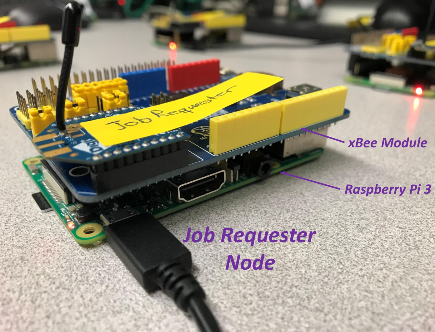
Shown in Fig. 7 is a setup mimicking a real-world scenario of mobile pipeline computing, where each Raspberry Pi 3 module integrated with a XBee module is used to represent either a requester or a worker. The wireless LAN interface (WiFi) on the raspberry Pi 3 devices has options IEEE 802.11 b/g/n, and 802.11n is used in this experiment to emulate D2D for transmitting wideband processed data. On the other hand, ZigBee22 2 ZigBee is a Home Area Network (HAN) protocol built upon the 802.15. 4 IEEE standard, whereas XBee is a brand name referring to a family of devices from Digi International that support a group of HAN protocols including ZigBee and its enhanced versions. communication protocol is dedicated for transmitting narrowband control messages. Each of worker and requester devices is linked to its previous and next devices using WiFi protocol, and the requester is connected to all the workers using ZigBee protocol.



IV-B Demonstration of Pipeline Computing
It is expected that by taking advantage of available spare computing resources, overall run time can be reduced. However this needs to be validated experimentally since an accurate outcome affected by various practical factors cannot be quantified theoretically. A small-scale deep learning task is tested on this setup by considering two types of operations: non-pipeline and pipeline operation making use of additional computing resources. In general, a computational process needs to be partitioned into subprocesses, and these subprocesses are sequentially arranged and assigned to distributed workers connected in a daisy-chain manner. Luckily, in Deep Neural Network (DNN) case, a computational process can be naturally divided into sequential subprocesses since a DNN structure is actually formed in a sequential manner (see Fig. 8). In non-pipeline operation (Case I in Fig. 8), there is only one worker node on which the whole LeNet DNN [lecun1998gradient] is implemented to classify the images, as shown in Fig. 8. In pipeline operation (Case II and Case III in Figs. 8 and 8, respectively), the LeNet DNN is distributed among the workers to classify the images in a coordinated way to increase process throughput.
| Case | # of workers | Total time (ms) | Throughput |
|---|---|---|---|
| I | One | 540.103 | 100% |
| II | Two | 347.780 | 155% |
| III | Three | 308.457 | 175% |
Shown in Table II is the testing result. When the LeNet DNN ran on one device (non-pipeline, Case I), it took a total time of about 540 ms to classify 100 images, where the total time includes processing time and communication time. To classify the same images using pipeline operation, with two and three workers it took about 348 ms and 308 ms, respectively. In other words, pipeline based LeNet DNN can increase classification throughput from 100% to 155% for two workers and to 175% for three workers. The experiment result agrees with our expectation that the more workers are involved the better performance is achieved. This experiment implies that pipeline computing on coordinated devices in a D2D-enable environment is feasible. Although this experiment has a limited scope, one can envision the same trend in performance improvement for different computation levels.
| Strategy | # of | Computing | Memory | Buffer | Bandwidth |
|---|---|---|---|---|---|
| score | workers | (MAC/s) | (kB) | (kB) | (kB/s) |
| 0.0989 | 2 | 0.0 | 0.0 | 0.0 | 1,834.0 |
| 10,164.7 | 15.6 | 313.6 | 4,361.0 | ||
| 15,363.1 | 4,427.0 | 1,382.4 | 60.0 | ||
| 0.2248 | 2 | 0.0 | 0.0 | 0.0 | 1,834.0 |
| 10,096.6 | 15.6 | 313.6 | 1,623.0 | ||
| 18,172.2 | 4,427.0 | 345.6 | 60.0 | ||
| 0.2511 | 2 | 0.0 | 0.0 | 0.0 | 1,834.0 |
| 18,872.9 | 257.6 | 313.6 | 1,721.0 | ||
| 5,925.0 | 4,185.0 | 409.6 | 60.0 | ||
| 0.3204 | 2 | 0.0 | 0.0 | 0.0 | 1,834.0 |
| 18,521.2 | 257.6 | 313.6 | 620.0 | ||
| 6,712.1 | 4,185.0 | 102.4 | 60.0 | ||
| 0.4107 | 2 | 0.0 | 0.0 | 0.0 | 1,834.0 |
| 16,188.2 | 3,341.6 | 313.6 | 471.0 | ||
| 3,522.6 | 1,101.0 | 48.0 | 60.0 | ||
| 0.4681 | 2 | 0.0 | 0.0 | 0.0 | 1,834.0 |
| 15,504.4 | 4,357.6 | 313.6 | 494.0 | ||
| 466.7 | 85.0 | 33.6 | 60.0 | ||
| 0.0759 | 3 | 0.0 | 0.0 | 0.0 | 1,834.0 |
| 10,096.6 | 15.6 | 313.6 | 1,472.0 | ||
| 30,317.7 | 242.0 | 345.6 | 621.0 | ||
| 6,716.1 | 4,185.0 | 102.4 | 60.0 | ||
| 0.1435 | 3 | 0.0 | 0.0 | 0.0 | 1,834.0 |
| 10,096.6 | 15.6 | 313.6 | 1,472.0 | ||
| 22,602.4 | 3,326.0 | 345.6 | 471.0 | ||
| 3,522.6 | 1,101.0 | 48.0 | 60,0 |
* MAC/s = Multiply-Accumulate/sec.
| Parameter | Description | Value |
| resource-weighting vector | (0.4, 0.25, 0.25, 0.1) | |
| weights on different powers | (0.3, 0.7, 0) | |
| of the adjacent matrix | ||
| weights on the three | (0.05, 0.5, 0.3) | |
| types of scores | ||
IV-C Computer Simulation
The effectiveness of our proposed path finding techniques is tested using computer simulation. A large number of parameters need to be specified for the simulation. Eight pipeline configuration strategies for a deep learning inference job are provided in Table III, where the preference scores are specified based on required resource consumptions, and the required resource consumptions is normalized before feeding into the algorithm. Three types of random variables (RVs) need to be considered: 1) link qualities, 2) node reliabilities, and 3) available resources. An exception is that the requester always sets its reliability level to the highest, i.e., one. For convenience, beta distribution is used to model the probability density functions (pdfs) of these RVs. A modeled pdf can be adjusted flexibly by tuning the two parameters and . For instance, as shown in Fig. 9, three probability distributions are mimicked using three different parameter pairs.

Essential performance metrics include (i) path score , (ii) , probability that at least one qualified path exists, and (iii) , edge reduction rate contributed by graph trimming. , and are affected by pool size (), link quality, node reliability, resource availability and required minimum resources, etc. Table IV shows some key parameters used in the simulation, where the values of and are taken such that , and are at comparable levels. How to select these parameters to accurately mimic the reality is beyond the scope of this paper. Instead, we consider two system settings for qualitative comparison: case 1 with relatively small pool size, poor condition and less resources, and case 2 with relatively large pool size, good condition and rich resources.

The winning strategy is strategy 6 which has a higher preference score, and the simulation results for the two cases are provided in Fig. 10. Obviously, Case-1 setting (poor condition) corresponds to a lower score () and worse chance of pipeline existence (). One can see that graph trimming (decrease of ) dose not cause noticeable degradation in the optimality (); and if is kept below 20%, the reduction in the chance of pipeline existence () is negligible. Note that a shorter pipeline is more likely selected than a longer one, since a shorter path is in favor of path quality and reliability; but the likelihood can be adjusted via assigning a higher strategy score () to a preferred strategy (). Furthermore, the amount of edge reduction can be tuned by changing the thresholds and/or .

V Stability Analysis of mmWave D2D Based Opportunistic Mobile Pipeline Computing
5G technology integrated with mmWave enables GHz-bandwidth transmission at millisecond-level latency. Since D2D is part of 5G, in the near future our proposed mobile pipeline computing can enjoy the advantage of large bandwidth and low-latency offered by 5G mmWave. However, mmWave communication is very sensitive to link blockage [32, 33, 34, 18], and the blockage effect will be amplified as multiple links have to be utilized simultaneously in the pipeline computing scenario. In mmWave communication, blockage is a dominating factor responsible for interruption of a communication session. Therefore, in performance analysis it is reasonable to ignore other possible factors that may make contribution to the interruption of a pipeline session. In this section we analyze the pipeline stability using a 2-state discrete-time Markov chain as a dynamic blockage model, assuming all links behave statistically identically and independently. In [18] the 2-state blockage model is validated based on measurement. The model includes two states called “Unshadowed” (or standing for Good) and “Shadowed” (or standing for Bad), along with a transition probability matrix. From a pipeline stability perspective, we are concerned about the following two parameters given that a pipeline has been formed:
- 1.
The probability of success (i.e., a computation job is not interrupted by blockage) for a given session time;
- 2.
The average number of attempts to form a pipeline for a requested computation job, assuming the statistic model keeps unchanged and the requester continues to request a pipeline computing session till the job is completed.
Let be the session time defined as a duration that starts upon a pipeline is formed and ends right after the computation job is completed, the required number of nodes (including both requester and workers) on a pipeline, the probability of success conditioned on that a pipeline is formed, () the sampling time interval of the dynamic blockage model, and the probability for transition from state to state , i.e., . Using the (1st-order) Markov chain property and denoting , is given by
| (7) | |||||
where stands for , or “event occurs consecutively for times”, and has been applied.
To increase the success probability, a straightforward strategy is to employ multiple pipelines concurrently (Fig. 11) at increased resource consumption, if these pipelines are available. When concurrently qualified pipelines are used to execute a job at the same time, assuming the pipelines are statistically independent, the success probability conditioned on that at least qualified pipelines are formed, denoted by , is given by
| (8) |
With , it is not difficult to derive the conditional average number of attempts denoted by ,
| (9) | |||||


Shown in Fig. 12 – Fig. 15 are evaluation results using some values provided in [18]: (being in [18] ms, (being in [18]. As expected, a shorter session time and/or a shorter pipeline lead to a better stability performance, and the use of concurrent multiple pipelines can improve the performance significantly at the cost of increased system resource consumption. Note that, to evaluate stability, all of these results are conditioned on that the pipelines are formed. Although , the prior probability that at least pipeline paths exist depends on multiple factors, it can be expected that this probability would approach one as the size of a mobile computing pool increases.
VI Conclusions
The mobile collaborative pipeline computing concept is proposed and studied. Our analytical and experimental results give us confidence on feasibly applying our proposed techniques to real world problems, such as deep learning inference on mobile devices in a D2D environment. Our proposed system should be suitable for real-time on-site computation-intensive tasks for which current cloud computing technology may not be suitable. Based on the foundation laid, further research and development are expected. Future work includes 1) extending single-request single-session service to multi-request multi-session service, considering uncertain resource availability [41, 42, 43], which resorts to optimum scheduling and system resource management to maximize the overall performance of a community computing pool; 2) improve the path finding framework by taking into account the impact of session time to maximize the success probability (and minimize at the same time); 3) performance evaluation considering realistic system setting and protocols; and 4) broad issues around computing pool management, such as worker trustworthiness, privacy of computation jobs and the job owners (requesters), and decentralized management.
References
- [1] Y.-D. Lin and Y.-C. Hsu, “Multihop cellular: A new architecture for wireless communications,” in Proceedings IEEE INFOCOM 2000. Conference on Computer Communications. Nineteenth Annual Joint Conference of the IEEE Computer and Communications Societies (Cat. No. 00CH37064), vol. 3. IEEE, 2000, pp. 1273–1282.
- [2] G. Fodor, E. Dahlman, G. Mildh, S. Parkvall, N. Reider, G. Miklós, and Z. Turányi, “Design aspects of network assisted device-to-device communications,” IEEE Communications Magazine, vol. 50, no. 3, pp. 170–177, 2012.
- [3] A. Pyattaev, K. Johnsson, A. Surak, R. Florea, S. Andreev, and Y. Koucheryavy, “Network-assisted D2D communications: Implementing a technology prototype for cellular traffic offloading,” in 2014 IEEE Wireless Communications and Networking Conference (WCNC). IEEE, 2014, pp. 3266–3271.
- [4] J. Qiao, X. S. Shen, J. W. Mark, Q. Shen, Y. He, and L. Lei, “Enabling device-to-device communications in millimeter-wave 5G cellular networks,” IEEE Communications Magazine, vol. 53, no. 1, pp. 209–215, 2015.
- [5] Z. Wu, V. D. Park, and J. Li, “Enabling device to device broadcast for LTE cellular networks,” IEEE Journal on Selected Areas in Communications, vol. 34, no. 1, pp. 58–70, 2016.
- [6] S.-Y. Lien, C.-C. Chien, F.-M. Tseng, and T.-C. Ho, “3GPP device-to-device communications for beyond 4G cellular networks,” IEEE Communications Magazine, vol. 54, no. 3, pp. 29–35, 2016.
- [7] M. A. Alim, T. Pan, M. T. Thai, and W. Saad, “Leveraging social communities for optimizing cellular device-to-device communications,” IEEE Transactions on Wireless Communications, vol. 16, no. 1, pp. 551–564, 2016.
- [8] A. Orsino, I. Farris, L. Militano, G. Araniti, S. Andreev, I. Gudkova, Y. Koucheryavy, and A. Iera, “Exploiting D2D communications at the network edge for mission-critical IoT applications,” in European Wireless 2017; 23th European Wireless Conference. VDE, 2017, pp. 1–6.
- [9] N. Giatsoglou, K. Ntontin, E. Kartsakli, A. Antonopoulos, and C. Verikoukis, “D2D-aware device caching in mmWave-cellular networks,” IEEE Journal on Selected Areas in Communications, vol. 35, no. 9, pp. 2025–2037, 2017.
- [10] R. I. Ansari, C. Chrysostomou, S. A. Hassan, M. Guizani, S. Mumtaz, J. Rodriguez, and J. J. Rodrigues, “5G D2D networks: Techniques, challenges, and future prospects,” IEEE Systems Journal, vol. 12, no. 4, pp. 3970–3984, 2017.
- [11] M. Haus, M. Waqas, A. Y. Ding, Y. Li, S. Tarkoma, and J. Ott, “Security and privacy in device-to-device (D2D) communication: A review,” IEEE Communications Surveys & Tutorials, vol. 19, no. 2, pp. 1054–1079, 2017.
- [12] G. H. Sim, A. Loch, A. Asadi, V. Mancuso, and J. Widmer, “5G millimeter-wave and D2D symbiosis: 60 GHz for proximity-based services,” IEEE Wireless Communications, vol. 24, no. 4, pp. 140–145, 2017.
- [13] Y. He, J. Ren, G. Yu, and Y. Cai, “D2D communications meet mobile edge computing for enhanced computation capacity in cellular networks,” IEEE Transactions on Wireless Communications, vol. 18, no. 3, pp. 1750–1763, 2019.
- [14] F. Boccardi, R. W. Heath Jr, A. Lozano, T. L. Marzetta, and P. Popovski, “Five disruptive technology directions for 5G,” arXiv preprint arXiv:1312.0229, 2013.
- [15] T. S. Rappaport, S. Sun, R. Mayzus, H. Zhao, Y. Azar, K. Wang, G. N. Wong, J. K. Schulz, M. Samimi, and F. Gutierrez, “Millimeter wave mobile communications for 5G cellular: It will work!” IEEE access, vol. 1, pp. 335–349, 2013.
- [16] M. Aazam, K. A. Harras, and S. Zeadally, “Fog computing for 5G tactile industrial internet of things: QoE-aware resource allocation model,” IEEE Transactions on Industrial Informatics, vol. 15, no. 5, pp. 3085–3092, 2019.
- [17] S. L. Cotton, W. G. Scanlon, and B. K. Madahar, “Millimeter-wave soldier-to-soldier communications for covert battlefield operations,” IEEE Comm. Magazine, vol. 47, no. 10, pp. 72–81, 2009.
- [18] G. R. MacCartney, T. S. Rappaport, and S. Rangan, “Rapid fading due to human blockage in pedestrian crowds at 5G millimeter-wave frequencies,” in IEEE GLOBECOM, 2017, pp. 1–7.
- [19] R. Duncan, “A survey of parallel computer architectures,” Computer, vol. 23, no. 2, pp. 5–16, 1990.
- [20] C. Pautasso and G. Alonso, “Parallel computing patterns for grid workflows,” in 2006 Workshop on Workflows in Support of Large-Scale Science. IEEE, 2006, pp. 1–10.
- [21] N. D. Lane, S. Bhattacharya, P. Georgiev, C. Forlivesi, L. Jiao, L. Qendro, and F. Kawsar, “Deepx: A software accelerator for low-power deep learning inference on mobile devices,” in Proceedings of the 15th International Conference on Information Processing in Sensor Networks. IEEE Press, 2016, p. 23.
- [22] S. Liu, Y. Lin, Z. Zhou, K. Nan, H. Liu, and J. Du, “On-demand deep model compression for mobile devices: A usage-driven model selection framework,” in Proceedings of the 16th Annual International Conference on Mobile Systems, Applications, and Services. ACM, 2018, pp. 389–400.
- [23] S. Andreev, V. Petrov, K. Huang, M. A. Lema, and M. Dohler, “Dense moving fog for intelligent IoT: Key challenges and opportunities,” IEEE Communications Magazine, vol. 57, no. 5, pp. 34–41, 2019.
- [24] T. Abdelzaher, N. Ayanian, T. Basar, S. Diggavi, J. Diesner, D. Ganesan, R. Govindan, S. Jha, T. Lepoint, B. Marlin et al., “Will distributed computing revolutionize peace? the emergence of battlefield IoT,” in 2018 IEEE 38th International Conference on Distributed Computing Systems (ICDCS). IEEE, 2018, pp. 1129–1138.
- [25] A. Giyenko and Y. Im Cho, “Intelligent UAV in smart cities using IoT,” in 2016 16th International Conference on Control, Automation and Systems (ICCAS). IEEE, 2016, pp. 207–210.
- [26] N. H. Motlagh, M. Bagaa, and T. Taleb, “UAV-based IoT platform: A crowd surveillance use case,” IEEE Communications Magazine, vol. 55, no. 2, pp. 128–134, 2017.
- [27] H. Kim and J. Ben-Othman, “A collision-free surveillance system using smart UAVs in multi domain IoT,” IEEE communications letters, vol. 22, no. 12, pp. 2587–2590, 2018.
- [28] G. Ding, Q. Wu, L. Zhang, Y. Lin, T. A. Tsiftsis, and Y.-D. Yao, “An amateur drone surveillance system based on the cognitive internet of things,” IEEE Communications Magazine, vol. 56, no. 1, pp. 29–35, 2018.
- [29] J. Mao, X. Chen, K. W. Nixon, C. Krieger, and Y. Chen, “MoDNN: Local distributed mobile computing system for deep neural network,” in Design, Automation & Test in Europe Conference & Exhibition (DATE), 2017. IEEE, 2017, pp. 1396–1401.
- [30] J. Mao, Z. Yang, W. Wen, C. Wu, L. Song, K. W. Nixon, X. Chen, H. Li, and Y. Chen, “MeDNN: A distributed mobile system with enhanced partition and deployment for large-scale DNNs,” in Proceedings of the 36th International Conference on Computer-Aided Design. IEEE Press, 2017, pp. 751–756.
- [31] Z. Zhao, K. M. Barijough, and A. Gerstlauer, “Deepthings: Distributed adaptive deep learning inference on resource-constrained IoT edge clusters,” IEEE Transactions on Computer-Aided Design of Integrated Circuits and Systems, vol. 37, no. 11, pp. 2348–2359, 2018.
- [32] S. Collonge, G. Zaharia, and G. El Zein, “Influence of the human activity on wide-band characteristics of the 60 GHz indoor radio channel,” IEEE Trans. Wireless Comm., vol. 3, no. 6, 2004.
- [33] S. Singh, F. Ziliotto, U. Madhow, E. Belding, and M. Rodwell, “Blockage and directivity in 60 GHz wireless personal area networks: From cross-layer model to multihop MAC design,” IEEE Journal on Selected Areas in Communications, vol. 27, no. 8, pp. 1400–1413, 2009.
- [34] H. Jung and I.-H. Lee, “Connectivity analysis of millimeter-wave device-to-device networks with blockage,” International Journal of Antennas and Propagation, vol. 2016, 2016.
- [35] Y. Wang and J. Vassileva, “Trust and reputation model in peer-to-peer networks,” in Proceedings Third International Conference on Peer-to-Peer Computing (P2P2003). IEEE, 2003, pp. 150–157.
- [36] R. Chen, F. Bao, and J. Guo, “Trust-based service management for social internet of things systems,” IEEE transactions on dependable and secure computing, vol. 13, no. 6, pp. 684–696, 2016.
- [37] Y. Wang, “Trust quantification for networked cyber-physical systems,” IEEE Internet of Things Journal, vol. 5, no. 3, pp. 2055–2070, 2018.
- [38] L. Kjerengtrøen and P. H. Wirsching, “Structural reliability analysis of series systems,” Journal of Structural Engineering, vol. 110, no. 7, pp. 1495–1511, 1984.
- [39] N. E. Selinski, C. Rasmussen, M. Wawro, and M. Zandieh, “A method for using adjacency matrices to analyze the connections students make within and between concepts: The case of linear algebra,” Journal for Research in Mathematics Education, vol. 45, no. 5, pp. 550–583, 2014.
- [40] C. Mukherjee and G. Mukherjee, “Role of adjacency matrix in graph theory,” IOSR Journal of Computer Engineering, vol. 16, no. 2, pp. 58–63, 2014.
- [41] B. Javadi, D. Kondo, J.-M. Vincent, and D. P. Anderson, “Discovering statistical models of availability in large distributed systems: An empirical study of seti@ home,” IEEE Transactions on Parallel and Distributed Systems, vol. 22, no. 11, pp. 1896–1903, 2011.
- [42] D. Lázaro, D. Kondo, and J. M. Marquès, “Long-term availability prediction for groups of volunteer resources,” Journal of Parallel and Distributed Computing, vol. 72, no. 2, pp. 281–296, 2012.
- [43] B. Javadi, K. Matawie, and D. P. Anderson, “Modeling and analysis of resources availability in volunteer computing systems,” in 2013 IEEE 32nd International Performance Computing and Communications Conference (IPCCC). IEEE, 2013, pp. 1–9.
![[Uncaptioned image]](2006.09301v1/Terry_N_Guo.jpg) |
Terry N. Guo received his M.S. degree in telecommunications engineering from Beijing University of Posts and Telecommunications, Beijing, in 1990, and Ph.D. degree in communications and electronic systems from the University of Electronic Science and Technology of China, Chengdu, in 1997. From January 1997 to December 1999, he was a postdoctoral researcher at the Center for Wireless Communications, University of California, San Diego. He worked for a few startups in New Jersey in early 2000s. Since 2004, he has been with the Center for Manufacturing Research, Tennessee Technological University, Tennessee, playing a wide range of duties including research, teaching and laboratory management. He has been conducting research and prototyping research testbeds in the areas of wireless communications, Radio Frequency (RF) systems, wide band beamforming, statistic signal processing, and data analytics. His recent research interests include Internet of Things (IoT) security and privacy, smart manufacturing, 5G Device-to-Device (D2D) communications, and mobile opportunistic computing. |
![[Uncaptioned image]](2006.09301v1/a2.png) |
Hawzhin Mohammed received his B.Sc. degree in electrical engineering from Salahaddin University, Erbil, Iraq, in 2000. He received his M.Sc. degree from Tennessee Technological University, Cookeville, TN, USA, in 2017, where he is currently pursuing his Ph.D. degree at the Department of Electrical and Computer Engineering. His current research interest includes wireless network security, hardware security, IoT security, machine learning, and deep learning. |
![[Uncaptioned image]](2006.09301v1/a3.jpg) |
Syed Rafay Hasan received the B.Eng. degree in electrical engineering from the NED University of Engineering and Technology, Pakistan, and the M.Eng. and Ph.D. degrees in electrical engineering from Concordia University, Montreal, QC, Canada. From 2006 to 2009, he was an Adjunct Faculty Member with Concordia University. From 2009 to 2011, he was a Research Associate with the Ecole Polytechnique de Montreal. Since 2011, he has been with the Electrical and Computer Engineering Department, Tennessee Tech University, Cookeville, TN, USA, where he is currently an Associate Professor. He has published more than 69 peer-reviewed journal and conference papers. His current research interests include hardware design security in the Internet of Things (IoT), hardware implementation of deep learning, deployment of convolution neural networks in the IoT edge devices, and hardware security issues due to adversarial learning. He received the Postdoctoral Fellowship Award from the Scholarship Regroupment Stratgique en Microsystmes du Québec, SigmaXi Outstanding Research Award, Faculty Research Award from Tennessee Tech University, the Kinslow Outstanding Research Paper Award from the College of Engineering, Tennessee Tech University, and the Summer Faculty Fellowship Award from the Air force Research Lab (AFRL). He has received research and teaching funding from NSF, ICT-funds UAE, AFRL, and Intel Inc. He has been part of the funded research projects, as a PI or a Co-PI, that worth more than $1.1 million. He has been the Session Chair and Technical Program Committee Member of several IEEE conferences including ISCAS, ICCD, MWSCAS, and NEWCAS, and a Regular Reviewer for several IEEE Transactions and other journals including TCAS-II, IEEE ACCESS, Integration, the VLSI Journal, IET Circuit Devices and Systems, and IEEE Embedded System Letters. |