CC-Light eQASM Architecture Specification

X. Fu email: xiangfu@quanta.org.cn Affiliation: QuTech, Delft University of Technology

Date: May 2018

Abstract.

This document ¹¹ 1 The CC-Light eQASM is a joint effort of the team (X. Fu, L. Riesebos, J. van Someren, and J. van Straten) in QuTech. This specification is written by X. Fu. If eQASM or CC-Light is used in your work, please cite to the following paper:
X. Fu, L. Riesebos, M. A. Rol, J. van Straten, J. van Someren, N. Khammassi, I. Ashraf, R. F. L. Vermeulen, V. Newsum, K. K. L. Loh, J. C. de Sterke, W. J. Vlothuizen, R. N. Schouten, C. G. Almudever, L. DiCarlo, and K. Bertels, eQASM: An Executable Quantum Instruction Set Architecture, IEEE International Symposium on High Performance ComputerArchitecture (HPCA), pp.224-237, IEEE, 2019. is the specification of the CC-Light instantiation of executable QASM (eQASM), a quantum instruction set architecture (QISA) developed in QuTech targeting to control a seven-qubit superconducting quantum processor. This document can serve as a reference manual for low-level programmers, compiler backend developers, and microarchitecture implementers of eQASM. The design of CC-Light eQASM is under the Apache 2.0 License.

1. Introduction

Executable QASM (eQASM) is an executable Quantum Instruction Set Architecture (QISA) for the quantum accelerator in a heterogeneous architecture as proposed in (fu2018eqasm). eQASM contains both quantum instructions and auxiliary classical instructions. eQASM supports a set of discrete quantum operations which can be defined via configuration before runtime. eQASM features accurate timing, Single-Operation-Multiple-Qubit (SOMQ) execution, VLIW architecture, programmable runtime feedback, and operational implementation.

We instantiated eQASM targeting a seven-qubit superconducting quantum processor. Since the binary of this eQASM instantiation can be executed by a microarchitecture implemented in the device QuTech Central Controller-Light (CC-Light), we call this instantiation CC-Light eQASM to distinguish it from eQASM itself and other eQASM instantiation.

This document serves as a reference manual for both CC-Light users who write program at the QISA level and compiler developers who is going to develop backends for CC-Light eQASM instructions. Since the paper (fu2018eqasm) explains the eQASM architecture from a higher-level perspective, this document mostly focus on the specification of CC-Light eQASM to avoid redundancy.

This document is organized as following. An overview of the CC-Light eQASM is shown in Section 2. The formal eQASM assembly syntax is shown in Section 3. Section 4 presents the alphabet list of CC-Light eQASM instructions except the quantum bundle instructions. The appendix give some examples to illustrate how to use eQASM to perform quantum experiments and algorithms. Also, the format of the configuration file used to configure the assembler is given.

2. eQASM Overview

Similar to GPU or NPU, quantum computing can be integrated in a heterogeneous architecture as shown in Fig. 1. The quantum part can be seen as a coprocessor used to accelerate particular tasks. eQASM only describes computation tasks executed on the quantum coprocessor.

Refer to caption — Figure 1. Quantum processor as an accelerator in a heterogeneous architecture.

This section introduces the eQASM programming and compilation model, the quantum program lifecycle, the architectural state, and an overview of instructions.

2.1. Programming and Compilation Model

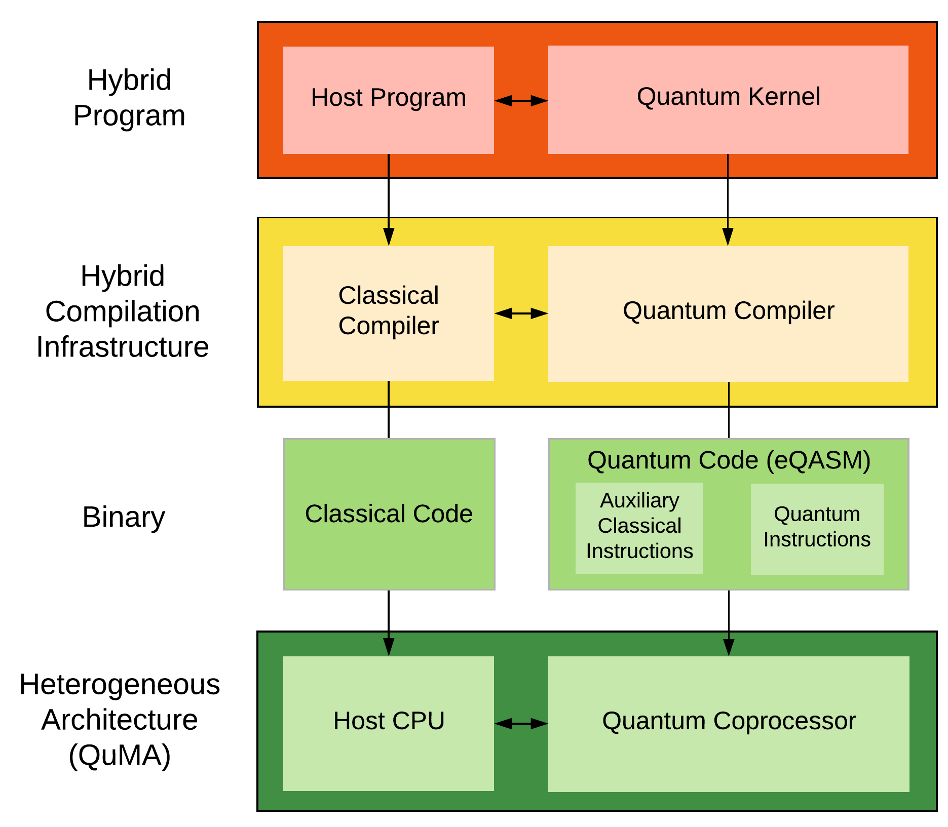
eQASM adopts the programming and compilation model as illustrated in Fig. 2. A quantum-classical hybrid program contains a host program and one or more quantum kernels. During execution, the host program invokes the quantum kernel(s) to accelerate a particular part of the computation. A hybrid compilation infrastructure compiles the hybrid program into classical code and quantum code which are fed to the heterogeneous architecture and directly executed by the host CPU and quantum coprocessor, respectively.

2.2. Quantum Program Lifecycle

A quantum program lifecycle using eQASM architecture contains the following phases: edit time, configuration time, compile time, and run time (or execution time).

2.2.1. Edit Time

In this phase, quantum programmers describe the quantum application or experiments using high-level languages. The host program can be described using a classical language, such as C++ or Python. The quantum kernel is described using a high-level quantum programming language, such as OpenQL. The host program should contain methods that offload the kernel to the accelerator for execution and read the result from the accelerator after the execution finishes. The current eQASM programming model does not define how these methods should be implemented.

2.2.2. Configuration Time

Since quantum instructions are not fully defined in eQASM, this phase is used to completely configure the instruction set and the hardware. This process contains the following aspects:

(1)

Define available pulses that can be applied on qubits, with each pulse corresponding to a primitive quantum operation (for single-qubit gates) or part of a primitive quantum operation (for two-qubit gates). Upload all these pulses into the codeword-triggered pulse generator of the microarchitecture and assign an unique codeword to each pulse. The duration of each operation can be calculated at this step.
(2)

Define i) all available quantum instructions and ii) the decomposition of each quantum instruction to the primitive quantum operations as defined in step (1). Each quantum instruction is assigned with an unique opcode. The decomposition is described by a map from one opcode to one or multiple codewords with correct timing. The duration of each operation calculated in step (1) is used to ensure correct timing.
(3)

Based on the opcode and decomposition defined in step (2), configure the assembler to translate each quantum instruction into a correct opcode, and the microcode unit in the microarchitecture to perform the correct decomposition.

2.2.3. Compile Time

In the hybrid compilation infrastructure, a conventional compiler, such as GNU Compilation Collection (GCC), compiles the host program into classical code. The quantum compiler, such as OpenQL (fu2017experimental), compiles the quantum kernels into quantum code consisting of eQASM instructions, which contains quantum instructions.

2.2.4. Run Time

The host program is executed on the host CPU. When the program execution reaches particular points, the host CPU loads the quantum code of the desired kernel as well as the necessary initialization data into the quantum coprocessor where the quantum code can be directly executed. After the kernel execution finishes, the quantum coprocessor writes the result into a shared memory space where the host CPU can fetch the result for the following processing. The current eQASM design does define the detailed mechanism of how host CPU and the quantum processor interacts.

2.3. Architectural State

As shown in Fig. 3, the architectural state of the quantum coprocessor includes: a data memory, an instruction memory, a program counter (PC), a general purpose register (GPR) file, comparison flags, a quantum operation target register file, timing and event queues, a qubit measurement result register file, an execution flag register file, and a quantum register file.

2.3.1. Data Memory

The data memory can buffer intermediate computation results and serve as the communication channel between the host CPU and the quantum coprocessor.

2.3.2. Instruction Memory & Program Counter

The eQASM instructions are stored in the instruction memory, and the Program Counter (PC) should contain the address of the next eQASM instruction to fetch.

2.3.3. General Purpose Registers

The general purpose register (GPR) file is a set of 32 registers, labeled as Ri, where $i\in\{0,1,\ldots,31\}$ is the register address. Each GPR is 32 bits wide.

2.3.4. Comparison Flags

The comparison flags store the comparison result of two general purpose registers which are used by comparison (CMP) and branch related instructions (BR, FBR). Table 1 lists the comparison flags with the corresponding meaning defined in eQASM. Function unsigned(Ri, 32) returns the 32-bit unsigned value stored in GPR Ri, and function signed(Ri, 32) returns the 32-bit signed value stored in GPR Ri. COMPFLAG represents the collection of all comparison flags. Each flag can be accessed using COMPFLAG.<flag> where <flag> is the name of the corresponding flag.

Table 1. Comparison flags defined in eQASM.

<Comparison Flag>	Meaning	<Comparison Flag>	Meaning
ALWAYS	1	NEVER	0
EQ	Rt == Rs	NE	Rt != Rs
LTU	unsigned(Rt) $<$ unsigned(Rs)	GEU	unsigned(Rt) $\geq$ unsigned(Rs)
LEU	unsigned(Rt) $\leq$ unsigned(Rs)	GTU	unsigned(Rt) $>$ unsigned(Rs)
LT	signed(Rt, 32) $<$ signed(Rs, 32)	GE	signed(Rt, 32) $\geq$ signed(Rs, 32)
LE	signed(Rt, 32) $\leq$ signed(Rs, 32)	GT	signed(Rt, 32) $>$ signed(Rs, 32)

2.3.5. Quantum Operation Target Registers

Each quantum operation target register can be used as an operand of a quantum operation. There are two types of quantum operation target registers: 32 single-qubit target registers for single-qubit operations, and 32 two-qubit target registers for two-qubit operations. A single- (two-)qubit target register is labelled as Si (Ti), where $i\in\{0,1,\ldots,31\}$ is the register address.

2.3.6. Timing and Event Queues

eQASM adopts a queue-based timing control scheme. The timing and event queues are used to buffer timing points and quantum operations generated from the execution of quantum instructions (see Section III-A of (fu2018eqasm)).

2.3.7. Qubit Measurement Result Registers

Each qubit is associated with a qubit measurement result register (QMRR) with each being 1 bit wide. Each QMRR stores the result of the last finished measurement instruction on the corresponding qubit when it is valid. It is labeled as Qi, where $i\in\{0,1,\ldots,6\}$ is the physical address of the qubit.

2.3.8. Execution Flag Registers

The execution flag register file contains an execution flag register for each qubit to support fast conditional execution. Each execution flag register contains four execution flags of which the values are derived automatically by the microarchitecture from the last measurement results of the corresponding qubit.

eQASM uses the following combinatorial logic to define each execution flag:

(1)

‘1’ (the default for unconditional execution);
(2)

‘1’ if and only if (iff) the last finished measurement result is $\ket{1}$ ;
(3)

‘1’ iff the last finished measurement result is $\ket{0}$ ;
(4)

‘1’ iff the last two finished measurements get the same result.

Note, the last finished measurement result refers to the result of the last finished measurement instruction on this qubit when these flags are used. It is irrelevant to the validity of the quantum measurement result register.

2.3.9. Quantum Register

The quantum register file is the collection of all seven physical qubits inside the quantum coprocessor. Each qubit is assigned a unique index, known as the physical address. Since data in qubits can be superposed, eQASM does not allow direct access to the data at the instruction level. Instead, users can measure qubits using measurement instructions and later access the results in the qubit measurement result registers.

2.4. Instruction Overview

Table 2. Overview of eQASM Instructions.

Type

Syntax

Description

Control

CMP Rs, Rt

Compare GPR Rs and Rt and store the result into the comparison flags.

BR <Comp. Flag>, Offset

Jump to PC + Offset if the specified comparison flag is ‘1’.

Data Transfer

FBR <Comp. Flag>, Rd

Fetch the specified comparison flag into GPR Rd.

LDI Rd, Imm

Rd = signed_ext(Imm[19..0], 32).

LDUI Rd, Imm, Rs

Rd = Imm[14..0]::Rs[16..0].

LD Rd, Rt(Imm)

Load data from memory address Rt + Imm into GPR Rd.

ST Rs, Rt(Imm)

Store the value of GPR Rs in memory address Rt + Imm.

FMR Rd, Qi

Fetch the result of the last measurement instruction on qubit i into GPR Rd.

Logical

AND/OR/XOR Rd, Rs, Rt

NOT Rd, Rt

Logical and, or, exclusive or, not.

Arithmetic

ADD/SUB Rd, Rs, Rt

Addition and subtraction.

Waiting

QWAIT Imm

QWAITR Rs

Specify a timing point by waiting for the number of cycles indicated by

the immediate value Imm or the value of GPR Rs.

Target Specify

SMIS Sd, <Qubit List>

SMIT Td, <Qubit Pair List>

Update the single- (two-)qubit operation target register Sd (Td).

Q. Bundle

[PI,] Q_Op [| Q_Op]*

Applying operations on qubits after waiting for a small number of

cycles indicated by PI.

An eQASM program can consist of quantum instructions and auxiliary classical instructions, which can be interleaved in the instruction memory. An overview of eQASM instructions is shown in Table 2. The top part of Table 2 contains the auxiliary classical instructions. There are four types: control, data transfer, logical and arithmetic instructions. These are all scalar instructions. The function sign_ext(Imm, 32) sign-extends the immediate value Imm to $32~\mathrm{bits}$ . The operator :: concatenates the two bit strings.

The bottom part of Table 2 contains the quantum instructions. There are three types of instructions:

•

Explicit waiting instructions used to specify timing points (QWAIT, QWAITR),
•

The quantum operation target register setting instructions (SMIS, SMIT), and
•

The quantum bundle instructions, which consist of the specification of a small waiting time and multiple quantum operations.

The next section shows the formal eQASM assembly syntax.

3. eQASM Assembly Syntax Specification

This section describes the eQASM assembly syntax.

3.1. File Organization

A single eQASM program should be written in a single assembly file which contains a sequence of lines. The following rules applies:

•

Each line ends with a newline character (ASCII CR+LF).
•

All characters are case insensitive, and extra blank is allowed between two identifiers.
•
User-defined identifiers can be used for mnemonic representations with the following rules:
- –
  
  They should start with a letter or an underscore, and followed by letters, digits, or underscores; and
- –
  
  They must not be a register name or an instruction name.
•
Immediate values can be specified in three different formats:
- –
  
  Plain format has no prefix and is interpreted as base-10 numbers. E.g., 23.
- –
  
  Hexadecimal format starts with the prefix 0x. E.g., 0x17.
- –
  
  Binary format starts with the prefix 0b. E.g., 0b10111.
•
Only line comment is supported.
- –
  
  It start with a hash mark (#) and continues to the end of the line.
•
A line can be an empty line, or a statement line.
- –
  
  An empty line is a line with only white space, which can be spaces, tabs, and/or comments.
- –
  
  The syntax of a statement line is defined in Section 3.2.

3.2. Statement

A statement line can contain one of the three kinds of statements:

•

A directive statement: a directive to the assembler that does not necessarily generate any code (see Section 3.3);
•

A label statement: a mnemonic representation of the address of the first instruction following the label (see Section 3.4); and/or
•

A machine operation statement: a single-format instruction or a quantum bundle (see Section 3.5) that generates one or multiple 32-bit instruction words.

Except that a label statement can be followed by a machine operation statement in the same line, not any two statements can be put in the same line.

3.3. Directive Statement

A directive can be a register alias or a constant alias. It is advised to put the directives at the top of a program.

3.3.1. Register aliases

Architecture registers can be given more meaningful names with the .register keyword:

⬇

1 .register <Register Name> <Alias Name>

where <Alias Name> should be a valid user-defined identifiers.

Example

The following code gives s7 the alias all_qubits, which indicates that s7 is going to be used to contain all seven qubits.

⬇

1 .register s7 all_qubits

2 SMIS s7, {0, 1, 2, 3, 4, 5, 6}

3 H all_qubits

3.3.2. Constant Alias

Numerical constants can be given a more meaningful name with the .def_sym keyword:

⬇

1 .def_sym <Alias Name> <Immediate>

where <Alias Name> should be a valid user-defined identifiers.

Example

The following code gives the constant 10000 the alias INIT_INTERVAL, which indicates an interval of $200~\mu\mathrm{s}$ when used by the QWAIT instruction.

⬇

1 .def_sym INIT_INTERVAL 10000

2 QWAIT INIT_INTERVAL

3.4. Label Statement

A label statement is a mnemonic representation of the address of the first instruction following the label. Labels can be used as the target of branch/jump instructions so that the programmer does not need to know the actual address of the target instruction.

Except blank, a label statement line starts with a label name followed by a colon. The label name should be a valid user-defined identifier. Every label should be unique across the eQASM program. A machine operation statement is allowed to be appended to a label statement in the same line.

Example 1:

⬇

1 Label: bs 1 X s0 # a label statement followed by a machine operation

2 # statement

3 ... # some other code here

4 goto Label # jump back

Example 2:

⬇

1 _AnotherValidLabel: # a label statement

2 bs 1 X s0 # a machine operation statement

3 ... # some other code here

4 goto _AnotherValidLabel # jump back

Example 1 and Example 2 are equivalent. The label Label or _AnotherValidLabel represents the address of the instruction bs 1 X s0. This label is then used by the goto instruction to form an infinite loop.

3.5. Machine Operation Statement

A machine operation statement can be a single-format instruction or a quantum bundle. A single instruction contains all auxiliary classical instructions, and the QWAIT, QWAITR, SMIS, or SMIT instruction, as shown in Table 2. Every single-format instruction is encoded into a single instruction word (32-bit). The syntax, encoding, and behavior of each instruction is presented in the alphabet list of instructions in Section 4.

The assembly format of a quantum bundle is defined as following with PI ranging from 0 to 7:

[PI,] <Quantum Operation> [| <Quantum Operation>]*

A quantum operation can be one of the three types as shown in table 3.

Quantum Operation Type	Syntax
No Operation	QNOP
Single-qubit	<single_qubit_operation_name> Si
Two-qubit	<two_qubit_operation_name> Ti

Table 3. Quantum operation types and the syntax.

A quantum bundle might be translated into one or multiple 32-bit quantum bundle instructions depending on if the number of quantum operations in the bundle is larger than 2 or not. The binary format of a quantum bundle instruction is shown in Table 4. The most significant bit (MSb) being ‘1’ means that this is a quantum bundle instruction instead of a single-format instruction whose MSb is ‘0’.

Table 5. Quantum bundle format.


31	30	29	28	27	26	25	24	23	22	21	20	19	18	17	16	15	14	13	12	11	10	9	8	7	6	5	4	3	2	1	0
1	q_opcode_0									Si/Ti_0					q_opcode_1									Si/Ti_1					PI

The single-qubit and two-qubit operation names and their opcodes are user-definable, which are specified using a configuration file qisa_opcodes.qmap. The file qisa_opcodes.qmap will be read by the assembler. The specification of qisa_opcodes.qmap is shown in Appendix B. The control store of the microcode unit (see (fu2018eqasm) for more details) should also be configured in a consistent way. The specification of the control store file used by the CC-Light driver and an example are shown in Appendix . Since the quantum opcode width is 9, the user can define at most 511 quantum operations except the QNOP operation during one run of the quantum operation.

3.6. Predefined Macros

The CC-Light assembler also includes some predefined MACROs to enable easy programming. For example, the instruction BLTU Rs,Rt, tgt_addr will be decomposed by the assembler to two separate instructions:

CMP Rs, Rt

BR LTU, tgt_addr

It first compares Rs and Rt, and changes the PC to the target address if unsigned(Rs) is less than unsigned(Rt).

Table 6 shows the predefined macros in CC-Light eQASM. Note, if one macro is decomposed into two instructions, then these two instructions will be put into two consecutive lines by the assembler.

Table 6. Predefined macros in CC-Light eQASM.

Macro	Intepretation	Comment
GOTO addr	BR always, addr	PC $\leftarrow$ addr $\ll$ 2
BRN addr	BR never, addr	No operation
BEQ Rs, Rt, addr	CMP Rs, Rt BR eq, addr
BNE Rs, Rt, addr	CMP Rs, Rt BR ne, addr
BLT Rs, Rt, addr	CMP Rs, Rt BR lt, addr
BLE Rs, Rt, addr	CMP Rs, Rt BR le, addr
BGT Rs, Rt, addr	CMP Rs, Rt BR gt, addr
BGE Rs, Rt, addr	CMP Rs, Rt BR ge, addr
BLTU Rs, Rt, addr	CMP Rs, Rt BR ltu, addr
BLEU Rs, Rt, addr	CMP Rs, Rt BR leu, addr
BGTU Rs, Rt, addr	CMP Rs, Rt BR gtu, addr
BGEU Rs, Rt, addr	CMP Rs, Rt BR geu, addr
MOV Rd, Rs	LDI Rd, 0 ADD Rd, Rs, Rd	Rd $\leftarrow$ Rs
SHL1 Rd, Rs	ADD Rd, Rs, Rs	Rd $\leftarrow$ Rs $\ll$ 1
MULT2 Rd, Rs	ADD Rd, Rs, Rs	Rd $\leftarrow$ Rs $\times$ 2
NAND Rd, Rs, Rt	AND Rd, Rs, Rt NOT Rd, Rd
NOR Rd, Rs, Rt	OR Rd, Rs, Rt NOT Rd, Rd
XNOR Rd, Rs, Rt	XOR Rd, Rs, Rt NOT Rd, Rd

3.7. Latency Between Instructions

It is a common case that a later instruction $k_{j}$ maybe depend on a previous instruction $k_{i}$ , i.e., the instruction $k_{j}$ needs to read the register which was previously written by $k_{i}$ . This is called data dependency.

QuMA_v2 is implemented in a pipelined fashion, and not all data dependency is resolved by the hardware. Instead, the compiler should be aware of this fact and insert a small number of independent instructions between two inter-dependent instruction to make sure the later one is reading the correct value. We call this process instruction latency compensation.

Two kinds of latency requires compensation: writing and reading comparison flags, writing and reading the measurement result (FMR). NOTE, any writing and reading the same GPRs are automatically handled by the microarchitecture, which requires no compensation. Also, No branch slot is reserved in the CC-Light eQASM, in other words, all instructions following a BR instruction will not be executed once the branch takes place.

3.7.1. Comparison Flags

One extra instruction is required between any instruction writing the comparison flags (cmp) and any instruction reading the comparison flags (fbr and br).

3.7.2. FMR

To enable the comprehensive feedback control work properly, two independent instructions should be inserted between any measurement instructions and the following FMR instruction, as shown in Fig. 4.

⬇

1 SMIS S0, {0}

2 SMIS S1, {1}

3 LDI R0, 1

4 MeasZ S1

5 QWAIT 30

6 NOP # two insns compensate for latency of MSMT -> FMR

7 FMR R1, Q1 # fetch msmt result

8 CMP R1, R0 # compare

9 NOP # one insn compensate for latency of CMP -> BR

10 BR EQ, eq_path # jump if R0 == R1

11 ne_path:

12 X S0 # happen if msmt result is 0

13 BR ALWAYS, continue

14 eq_path:

15 Y S0 # happen if msmt result is 1

16 continue:

17 ...

Figure 4. Conditionally performing a gate on qubit 0 based on the measurement result of qubit 1 using comprehensive feedback control. NOPs are inserted between dependent instructions.

4. Alphabet List of Predefined eQASM Instructions

In this section, We start by defining some basic functions using pseudo code, which are used in describing the behavior of instructions. The alphabet list of the predefined eQASM instructions are given in the following subsection.

4.1. Numbering & Operators

In CC-Light eQASM, binary data is Most Significant bit (MSb) first (i.e. the MSb is on the left side of the bit string) and “LSb 0” bit numbering (i.e., the Least Significant bit (LSb) is numbered as 0). For example, the constant 0x5 is represented as 0b00000101 in a eight-bit binary representation, and bit 0 is of the value ‘1’.

Table 7 defines the operators used in the instruction description.

Table 7. Operators with the meaning and precedence used in this manual. Note, a smaller number indicates a higher precedence.

Operator

Meaning

Precedence

{\small\texttt{bitstr}}\left[{\small\texttt{h}}:{\small\texttt{l}}\right]

Slice the bit string bitstr, with the range from the h-th bit down to the l-th bit.

\left[{\small\texttt{start}}..{\small\texttt{incr}}..{\small\texttt{end}}\right]

Generate an iterable list with a step of incr which starts from start and ends no

greater than end.

Exponent - left operand raised to the power of right

Bitwise NOT the operand

Multiply two operands

Divide left operand by the right one

Modulus - remainder of the division of left operand by the right

Add two operands or unary plus

Subtract right operand from the left or unary minus

\ll

Left shift the left operand by the number of bits specified by the right operand

\geq,~>,~\leq,~<

Relational operators

==,!=

Relational operators

Bitwise AND two operands

\wedge

Bitwise XOR two operands

|

Bitwise OR two operands

\leftarrow

assignment

4.2. Functions

4.2.1. Memory, Registers and Comparison Flags

Function MemByte(bitstring<32> x) returns the memory unit (MemUnit) with 8 bits whose address specified by the bit string x, and function MemByte_val(bitstring<32> x) further returns the 8-bit value stored in the byte structure. Function MemWord(bitstring<32> x) returns the word structure with the starting address specified by the bit string x, and function MemWord_val(bitstring<32> x) further returns the 32-bit value stored in the word structure.

⬇

MemUnit<1> MemByte(bitstring<32> x):

return Mem[unsigned_integer(x, 32)]

bitstring MemByte_val(bitstring<32> x):

return bitstring<8>(MemByte(x))

MemUnit<4> MemWord(bitstring<32> x):

return Mem[unsigned_integer(x, 32) + 3 : unsigned_integer(x, 32)]

bitstring MemWord_val(bitstring<32> x):

return bitstring<32>(MemWord(x))

Function GPR(bitstring<5> x) returns the general purpose register with the register number specified by the bit string x, and function GPR_val(bitstring<5> x) further returns the 32-bit value stored in the register.

⬇

return GPRF[unsigned_integer(x, 5)]

bitstring GPR_val(bitstring<5> x):

return bitstring<32>(GPR(x))

Function QOTRS(bitstring<5> x) (QOTRT(bitstring<5> x)) returns the single- (two-)qubit quantum operation target register with the register number specified by the bit string x, and function QOTRS_val(bitstring<5> x) (QOTRT_val(bitstring<5> x)) further returns the 7- (16-)bit value stored in the register.

⬇

return QOTRFS[unsigned_integer(x, 5)]

bitstring QOTRS_val(bitstring<5> x):

return bitstring<7>(QOTRS(x))

return QOTRFT[unsigned_integer(x, 5)]

bitstring QOTRT_val(bitstring<5> x):

return bitstring<16>(QOTRT(x))

Function QMRR(bitstring<3> x) returns the quantum measurement result register with the register number specified by the bit string x, and function QMRR_val(bitstring<5> x) further returns the 1-bit value stored in the register.

⬇

return QMRRF[unsigned_integer(x, 3)]

bitstring QMRR_val(bitstring<5> x):

return bitstring<1>(QMRR(x))

Function CompFlag_val returns the value of the comparison flag comp_flag. All comparison flags in CC-Light eQASM is listed in Table 1.

⬇

bitstring CompFlag_val(comp_flag):

return bitstring<1>(COMPFLAG.comp_flag)

4.2.2. UInt (Unsigned Int)

This function returns the unsigned value of the least significant N bits in the bit string x.

⬇

integer UInt(bitstring<M> x, integer N):

assert(M

\geq

integer result

\leftarrow{}

for i in [0 .. 1 .. (N - 1)]:

if x[i]

\leftarrow{}

\leftarrow{}

’1’:

result

\leftarrow{}

result + 2 ** i

end if

end for

return result

4.2.3. SInt (Signed Int)

This function returns the signed value of the least significant N bits in the bit string x.

⬇

integer SInt(bitstring<M> x, integer N):

assert(M

\geq

integer result

\leftarrow{}

for i in [0 .. 1 .. (N - 2)]:

if x[i]

\leftarrow{}

\leftarrow{}

’1’:

result

\leftarrow{}

result + 2 ** i

end if

end for

if x[N - 1]

\leftarrow{}

\leftarrow{}

’1’:

result

\leftarrow{}

result - 2 ** (N - 1)

end if

return result

4.2.4. ToUBitStr (Convert Unsigned Integer to Bit String)

This function returns the N-bit binary representation of the given unsigned integer int_val.

⬇

bitstring ToUBitStr(integer int_val, integer N):

assert(0

\leq

int_val

\leq

2 ** N - 1)

bitstring<N> result

\leftarrow{}

if int_val > 2 ** (N -1):

result[N - 1]

\leftarrow{}

int_val

\leftarrow{}

int_val - 2 ** (N - 1)

end if

for i in [0 .. 1 .. (N - 2)]:

result[i]

\leftarrow{}

int_val % 2

int_val

\leftarrow{}

(int_val - result[i]) / 2

end for

return result

4.2.5. ToSBitStr (Convert Signed Integer to Bit String)

This function returns the N-bit 2’s complement of the given signed integer int_val.

⬇

bitstring ToSBitStr(integer int_val, integer N):

assert(-2 ** (N - 1)

\leq

int_val

\leq

2 ** (N - 1) - 1)

bitstring<N> result

\leftarrow{}

if signed:

if int_val < 0:

result[N - 1]

\leftarrow{}

int_val

\leftarrow{}

int_val + 2 ** N

end if

for i in [0 .. 1 .. (N - 2)]:

result[i]

\leftarrow{}

int_val % 2

int_val

\leftarrow{}

(int_val - result[i]) / 2

end for

return result

4.2.6. ZeroExt (Unsigned Extend)

This function unsigned-extends the given bitstring x to the given length N.

⬇

bitstring ZeroExt(bitstring<M> x, integer N):

assert(M

\leq

bitstring<N> result

\leftarrow{}

result[0 : M - 1]

\leftarrow{}

x[0 : M - 1]

for i in [M, M + 1, ..., N - 1]:

result[i]

\leftarrow{}

end for

return result

4.2.7. SignExt (Signed Extend)

This function signed-extends the given bit string x to the given length N.

⬇

bitstring SignExt(bitstring<M> x, integer N):

assert(M

\leq

bitstring<N> result

\leftarrow{}

result[0 : M - 1]

\leftarrow{}

x[0 : M - 1]

for i in [M .. 1 .. (N - 1)]:

result[i]

\leftarrow{}

x[M - 1]

end for

return result

4.3. ADD – Add


31	30	29	28	27	26	25	24	23	22	21	20	19	18	17	16	15	14	13	12	11	10	9	8	7	6	5	4	3	2	1	0
0	0	1	1	1	1	0	Rd					Rs					Rt					reserved

Format: ADD Rd, Rs, Rt

Description:

The ADD instruction adds two GPR (Rs, Rt) values, and writes the result to the destination GPR (Rd) .

Operation:

⬇

integer sum

\leftarrow{}

UInt(GPR_val(Rs), 32) + UInt(GPR_val(Rt), 32)

GPR(Rd)

\leftarrow{}

ToUBitStr(sum, 32)

\leftarrow{}

PC + 4

# NOTE, with 2’s complement binary, it is the same for signed addition.

4.4. AND – And


31	30	29	28	27	26	25	24	23	22	21	20	19	18	17	16	15	14	13	12	11	10	9	8	7	6	5	4	3	2	1	0
0	0	1	1	0	1	0	Rd					Rs					Rt					reserved

Format: AND Rd, Rs, Rt

Description:

The AND instruction performs a bitwise AND of two GPR (Rs, Rt) values and writes the result to the destination GPR Rd.

Operation:

⬇

GPR(Rd)

\leftarrow{}

GPR_val(Rs) & GPR_val(Rt)

\leftarrow{}

PC + 4

4.5. BR – Branch


31	30	29	28	27	26	25	24	23	22	21	20	19	18	17	16	15	14	13	12	11	10	9	8	7	6	5	4	3	2	1	0
0	0	0	0	0	0	1	imm21																					comp_flag

Format: BR <comp_flag>, <label>

Description:

If the specified comparison flag is ‘1’, the BR instruction changes the PC by adding an immediate offset to it. Table 1 lists all allowed comparison flags and the corresponding meaning in eQASM. <label> points to the target instruction. The assembler is responsible for converting the <label> to the immediate value Imm21 according to the relative position of the target instruction and this BR instruction.

Operation:

⬇

if CompFlag_val(comp_flag)

\leftarrow{}

\leftarrow{}

’1’:

integer signed_sum

\leftarrow{}

SInt(PC, 17) + SInt(Imm21[14:0] << 2, 17)

\leftarrow{}

ToSBitStr(signed_sum, 18)[16:0]

end if

4.6. CMP – Compare


31	30	29	28	27	26	25	24	23	22	21	20	19	18	17	16	15	14	13	12	11	10	9	8	7	6	5	4	3	2	1	0
0	0	0	1	1	0	1	reserved					Rs					Rt					reserved

Format: CMP Rs, Rt

Description:

The CMP instruction compares the value of two GPRs (Rs, Rt), and updates the comparison flags based on the results.

Operation:

⬇

COMPFLAG.ALWAYS

\leftarrow{}

COMPFLAG.NEVER

\leftarrow{}

COMPFLAG.EQ

\leftarrow{}

(GPR_val(Rt)

\leftarrow{}

\leftarrow{}

GPR_val(Rs))

COMPFLAG.NE

\leftarrow{}

(GPR_val(Rt)

\neq

GPR_val(Rs))

COMPFLAG.LTU

\leftarrow{}

(UInt(GPR_val(Rt), 32) < UInt(GPR_val(Rs), 32))

COMPFLAG.GEU

\leftarrow{}

(UInt(GPR_val(Rt), 32)

\geq

UInt(GPR_val(Rs), 32))

COMPFLAG.LEU

\leftarrow{}

(UInt(GPR_val(Rt), 32)

\leq

UInt(GPR_val(Rs), 32))

COMPFLAG.GTU

\leftarrow{}

(UInt(GPR_val(Rt), 32) > UInt(GPR_val(Rs), 32))

COMPFLAG.LT

\leftarrow{}

(SInt(GPR_val(Rt), 32) < SInt(GPR_val(Rs), 32))

COMPFLAG.GE

\leftarrow{}

(SInt(GPR_val(Rt), 32)

\geq

SInt(GPR_val(Rs), 32))

COMPFLAG.LE

\leftarrow{}

(SInt(GPR_val(Rt), 32)

\leq

SInt(GPR_val(Rs), 32))

COMPFLAG.GT

\leftarrow{}

(SInt(GPR_val(Rt), 32) > SInt(GPR_val(Rs), 32))

\leftarrow{}

PC + 4

4.7. FBR – Fetch Branch Register (Comparison Flag)


31	30	29	28	27	26	25	24	23	22	21	20	19	18	17	16	15	14	13	12	11	10	9	8	7	6	5	4	3	2	1	0
0	0	1	0	1	0	0	Rd					reserved																comp_flag

Format: FBR <comp_flag>, Rd

Description:

The FBR instruction fetches the value of the given comparison flag comp_flag and writes it to the destination GPR Rd. Table 1 lists all allowed comparison flags and the corresponding meaning in eQASM.

Operation:

⬇

GPR(Rd)

\leftarrow{}

ZeroExt(CompFlag_val(comp_flag), 32)

\leftarrow{}

PC + 4

4.8. FMR – Fetch Measurement Result


31	30	29	28	27	26	25	24	23	22	21	20	19	18	17	16	15	14	13	12	11	10	9	8	7	6	5	4	3	2	1	0
0	0	1	0	1	0	1	Rd					reserved																	Qi

Format: FMR Rd, Qi

Description:

The FMR instruction fetches the measurement result of the last measurement instruction on qubit i and writes it to the destination GPR Rd.

Operation:

⬇

Wait until the last measurement instruction on qubit \code{i} finishes, i.e., the qubit measurement result register \code{Qi} gets valid, then perform the following:

GPR(Rd)

\leftarrow{}

ToUBitStr(Qi, 32)

\leftarrow{}

PC + 4

4.9. LD – Load Word from Memory


31	30	29	28	27	26	25	24	23	22	21	20	19	18	17	16	15	14	13	12	11	10	9	8	7	6	5	4	3	2	1	0
0	0	0	1	0	0	1	Rd					reserved					Rt					imm10

Format: LD Rd, Rt(Imm10)

Description:

The LD instruction loads the word from the memory address specified by the register Rt with an offset Imm10 into the destination GPR Rd.

Operation:

⬇

GPR(Rd)

\leftarrow{}

MemWord_val(UInt(GPR_val(Rt), 32) + SignExt(Imm10, 32))

\leftarrow{}

PC + 4

4.10. LDI – Load Immediate


31	30	29	28	27	26	25	24	23	22	21	20	19	18	17	16	15	14	13	12	11	10	9	8	7	6	5	4	3	2	1	0
0	0	1	0	1	1	0	Rd					imm20

Format: LDI Rd, Imm20

Description:

The LDI instruction loads the signed immediate value Imm20 into the destination GPR Rd.

Operation:

⬇

GPR(Rd)

\leftarrow{}

SignExt(Imm20, 32)

\leftarrow{}

PC + 4

4.11. LDUI – Load Unsigned Immediate


31	30	29	28	27	26	25	24	23	22	21	20	19	18	17	16	15	14	13	12	11	10	9	8	7	6	5	4	3	2	1	0
0	0	1	0	1	1	1	Rd					Rs					imm15

Format: LDUI Rd, Rs, Imm15

Description:

The LDUI instruction inserts an 15-bit constant into the upper 15 bits of the destination GPR Rd.

Operation:

⬇

GPR(Rd)

\leftarrow{}

Imm15 << 17 | GPR_val(Rs)[16:0]

\leftarrow{}

PC + 4

4.12. NOP – No Operation


31	30	29	28	27	26	25	24	23	22	21	20	19	18	17	16	15	14	13	12	11	10	9	8	7	6	5	4	3	2	1	0
0	0	0	0	0	0	0	0	0	0	0	0	0	0	0	0	0	0	0	0	0	0	0	0	0	0	0	0	0	0	0	0

Format: NOP

Description:

The NOP instruction performs no operation.

Operation:

⬇

\leftarrow{}

PC + 4

4.13. NOT – Not


31	30	29	28	27	26	25	24	23	22	21	20	19	18	17	16	15	14	13	12	11	10	9	8	7	6	5	4	3	2	1	0
0	0	1	1	0	1	1	Rd					reserved					Rt					reserved

Format: NOT Rd, Rt

Description:

The NOT instruction performs a bitwise NOT of a GPR (Rt) value and writes the result to the destination GPR Rd.

Operation:

⬇

GPR(Rd)

\leftarrow{}

~GPR_val(Rt)

\leftarrow{}

PC + 4

4.14. OR – Or


31	30	29	28	27	26	25	24	23	22	21	20	19	18	17	16	15	14	13	12	11	10	9	8	7	6	5	4	3	2	1	0
0	0	1	1	0	0	0	Rd					Rs					Rt					reserved

Format: OR Rd, Rs, Rt

Description:

The OR instruction performs a bitwise OR of two GPR (Rs, Rt) values and writes the result to the destination GPR Rd.

Operation:

⬇

GPR(Rd)

\leftarrow{}

GPR_val(Rs) | GPR_val(Rt)

\leftarrow{}

PC + 4

4.15. QWAIT – Quantum Wait Immediate


31	30	29	28	27	26	25	24	23	22	21	20	19	18	17	16	15	14	13	12	11	10	9	8	7	6	5	4	3	2	1	0
0	1	0	0	0	0	0	reserved					Imm20

Format: QWAIT Imm20

Description:

The QWAIT instruction creates a new timing point with a new timing label which is Imm20 cycles later than the previous timing point.

Operation:

⬇

TimingLabel

\leftarrow{}

TimingLabel + 1

TimingQueue.push(TimingLabel, Imm20)

\leftarrow{}

PC + 4

4.16. QWAITR – Quantum Wait Register


31	30	29	28	27	26	25	24	23	22	21	20	19	18	17	16	15	14	13	12	11	10	9	8	7	6	5	4	3	2	1	0
0	1	0	0	0	0	1	reserved					Rs					reserved

Format: QWAITR Rs

Description:

The QWAITR instruction creates a new timing point with a new timing label which is $k$ cycles later than the previous timing point. $k$ is an unsigned value specified by the 20 least significant bits of GPR Rs.

Operation:

⬇

TimingLabel

\leftarrow{}

TimingLabel + 1

TimingQueue.push(TimingLabel, GPR_val(Rs)[19:0])

\leftarrow{}

PC + 4

4.17. SMIS – Set Mask Immediate for Singe-qubit Operations


31	30	29	28	27	26	25	24	23	22	21	20	19	18	17	16	15	14	13	12	11	10	9	8	7	6	5	4	3	2	1	0
0	1	0	0	0	0	0	Sd						reserved												Imm7

Format: SMIS Sd, <Qubit List>

where, <Qubit List> has the following format:

{<qubit address>[, <qubit address>]*}

Description:

In CC-Light eQASM, the single-qubit target registers use a mask format in the binary. Each bit in the mask of the value ‘1’ indicates that the corresponding qubit is selected (see Fig. 5). The SMIS instruction sets the single-qubit quantum operation target register Sd to the mask which selects all qubits as listed in the set <Qubit List>. The assembler is responsible for translating <Qubit List> into the mask Imm7.

Operation:

⬇

QOTRS(Sd)

\leftarrow{}

Imm7

\leftarrow{}

PC + 4

Figure 5. The ordering of individual qubits and allowed qubit pairs.

4.18. SMIT – Set Mask Immediate for Two-qubit Operations


31	30	29	28	27	26	25	24	23	22	21	20	19	18	17	16	15	14	13	12	11	10	9	8	7	6	5	4	3	2	1	0
0	1	0	1	0	0	0	Td						reserved			Imm16

Format: SMIT Td, <Qubit Pair List>

where, <Qubit Pair List> has the following format:

{<Qubit Pair>[, <Qubit Pair>]*}

where, <Qubit Pair> has the following format:

(<Source Qubit Address>, <Target Qubit Address>)

Description:

In CC-Light eQASM, the two-qubit target registers use a mask format in the binary. Each bit in the mask of the value ‘1’ indicates one of 16 allowed qubit pairs selected (see Fig. 5). The SMIT instruction sets the two-qubit quantum operation target register Td to the mask which selects all allowed qubit pairs as listed in the set <Qubit Pair List>. The assembler is responsible for translating <Qubit Pair List> into the mask Imm16.

Operation:

⬇

QOTRT(Td)

\leftarrow{}

Imm16

\leftarrow{}

PC + 4

4.19. ST – Store Word to Memory


31	30	29	28	27	26	25	24	23	22	21	20	19	18	17	16	15	14	13	12	11	10	9	8	7	6	5	4	3	2	1	0
0	0	0	1	0	1	0	reserved					Rs					Rt					imm10

Format: ST Rs, Rt(Imm10)

Description:

The ST instruction stores the value of GPR Rs to the memory address specified by the register Rt with an offset Imm10.

Operation:

⬇

MemWord(UInt(GPR_val(Rt), 32) + SignExt(Imm10, 32))

\leftarrow{}

GPR_val(Rs)

\leftarrow{}

PC + 4

4.20. STOP – Stop


31	30	29	28	27	26	25	24	23	22	21	20	19	18	17	16	15	14	13	12	11	10	9	8	7	6	5	4	3	2	1	0
0	0	0	1	0	0	0	reserved

Format: STOP

Description:

The STOP instruction sets the execution flag STOP, and repeats executing itself infinitely. In other words, it stops the processor.

Operation:

⬇

EXEFLAG.STOP

\leftarrow{}

\leftarrow{}

4.21. SUB – Subtraction


31	30	29	28	27	26	25	24	23	22	21	20	19	18	17	16	15	14	13	12	11	10	9	8	7	6	5	4	3	2	1	0
0	0	1	1	1	1	1	Rd					Rs					Rt					reserved

Format: SUB Rd, Rs, Rt

Description:

The SUB instruction subtract a GPR (Rs) value from another GPR (Rt) value, and writes the result to the destination GPR (Rd).

Operation:

⬇

integer sum

\leftarrow{}

UInt(GPR_val(Rs), 32) + UInt(NOT(GPR_val(Rt)), 32) + UInt(1, 32)

GPR(Rd)

\leftarrow{}

ToUBitStr(sum, 32)

\leftarrow{}

PC + 4

# NOTE, with 2’s complement binary, it is the same for signed subtraction.

4.22. XOR – Exclusive Or


31	30	29	28	27	26	25	24	23	22	21	20	19	18	17	16	15	14	13	12	11	10	9	8	7	6	5	4	3	2	1	0
0	0	1	1	0	0	1	Rd					Rs					Rt					reserved

Format: XOR Rd, Rs, Rt

Description:

The XOR instruction performs a bitwise XOR of two GPR (Rs, Rt) values and writes the result to the destination GPR Rd.

Operation:

⬇

GPR(Rd)

\leftarrow{}

GPR_val(Rs) ^ GPR_val(Rt)

\leftarrow{}

PC + 4

References

(1) X. Fu, L. Riesebos, M. A. Rol, J. van Straten, J. van Someren, N. Khammassi, I. Ashraf, R. F. L. Vermeulen, V. Newsum, K. K. L. Loh, J. C. de Sterke, W. J. Vlothuizen, R. N. Schouten, C. G. Almudever, L. DiCarlo, and K. Bertels, “eQASM: An Executable Quantum Instruction Set Architecture,” in Proceedings of 25th IEEE International Symposium on High-Performance Computer Architecture (HPCA’19). IEEE, 2019, pp. 224–237.
(2) X. Fu, M. A. Rol, C. C. Bultink, J. van Someren, N. Khammassi, I. Ashraf, R. F. L. Vermeulen, J. C. de Sterke, W. J. Vlothuizen, R. N. Schouten, C. G. Almudever, L. DiCarlo, and K. Bertels, “An experimental microarchitecture for a superconducting quantum processor,” in Proceedings of the 50th Annual IEEE/ACM International Symposium on Microarchitecture (MICRO-50). ACM, 2017, pp. 813–825.

Appendix A Examples

In this section, we give some examples to show how to use eQASM to describe some quantum experiments and quantum algorithms.

A.1. Quantum Experiments

eQASM targets nowadays and near-term devices. Since calibration occupies most of the time when the quantum chip is being used, eQASM should also support the quantum experiments to calibrate qubits. This subsection shows the eQASM program of some widely-used quantum experiments, including $T_{1}$ , Rabi, AllXY, etc.

A.1.1. $T_{1}$

In this experiment, the CTPG only requires the $X$ pulse being uploaded.

⬇

1 .def_sym init_waiting_time 10000

2 .def_sym msmt_duration 15

4 .register r0 num_repitition

5 .register r1 max_repitition

6 LDI max_repitition, 10000

8 .register r3 start_interval

9 LDI start_interval, 50 # 1 us

11 .register r2 sweep_step

12 LDI sweep_step, 50 # 1 us

14 .register r4 max_interval

15 LDI max_interval, 5000 # 100 us

17 .register r5 round_interval

19 .register r31 constant_one

20 LDI constant_one, 1

22 SMIS S0, {0}

23 LDI num_repitition, 0

24 Round_Start:

25 LDI round_interval, start_interval

27 iteration_start:

28 QWAIT init_waiting_time

29 X S0

30 QWAITR round_interval

31 MEASZ S0

33 # go to next iteration if not reaching the maximal interval

34 add round_interval, round_interval, sweep_step

35 CMP round_interval, max_interval

36 NOP

37 BR LTU, iteration_start

39 add num_repitition, num_repitition, constant_one

41 # go to next round if the repition is insufficient

42 CMP num_repitition, max_repitition

43 NOP

44 BR LTU, round_start

A.1.2. Rabi

In this experiment, the CTPG should be uploaded with multiple variants of the $X$ gate, with each variant of a particular amplitude.

⬇

1 .def_sym init_waiting_time 10000

2 .def_sym msmt_duration 15

4 .register r0 num_repitition

5 .register r1 max_repitition

6 LDI max_repitition, 1000

8 .register r31 constant_one

9 LDI constant_one, 1

11 SMIS S0, {0}

12 LDI num_repitition, 0

14 Round_Start:

15 QWAIT init_waiting_time

16 X_Amp_0 S0

17 QWAITR round_interval

18 MEASZ S0

20 QWAIT init_waiting_time

21 X_Amp_1 S0

22 QWAITR round_interval

23 MEASZ S0

24 # not showing the following 37 iterations here

26 QWAIT init_waiting_time

27 X_Amp_2 S0

28 QWAITR round_interval

29 MEASZ S0

31 QWAIT init_waiting_time

32 X_Amp_3 S0

33 QWAITR round_interval

34 MEASZ S0

36 QWAIT init_waiting_time

37 X_Amp_4 S0

38 QWAITR round_interval

39 MEASZ S0

41 QWAIT init_waiting_time

42 X_Amp_5 S0

43 QWAITR round_interval

44 MEASZ S0

46 QWAIT init_waiting_time

47 X_Amp_6 S0

48 QWAITR round_interval

49 MEASZ S0

51 QWAIT init_waiting_time

52 X_Amp_7 S0

53 QWAITR round_interval

54 MEASZ S0

56 QWAIT init_waiting_time

57 X_Amp_8 S0

58 QWAITR round_interval

59 MEASZ S0

61 QWAIT init_waiting_time

62 X_Amp_9 S0

63 QWAITR round_interval

64 MEASZ S0

66 QWAIT init_waiting_time

67 X_Amp_10 S0

68 QWAITR round_interval

69 MEASZ S0

71 QWAIT init_waiting_time

72 X_Amp_11 S0

73 QWAITR round_interval

74 MEASZ S0

76 QWAIT init_waiting_time

77 X_Amp_12 S0

78 QWAITR round_interval

79 MEASZ S0

81 QWAIT init_waiting_time

82 X_Amp_13 S0

83 QWAITR round_interval

84 MEASZ S0

86 QWAIT init_waiting_time

87 X_Amp_14 S0

88 QWAITR round_interval

89 MEASZ S0

91 QWAIT init_waiting_time

92 X_Amp_15 S0

93 QWAITR round_interval

94 MEASZ S0

96 QWAIT init_waiting_time

97 X_Amp_16 S0

98 QWAITR round_interval

99 MEASZ S0

100

101 QWAIT init_waiting_time

102 X_Amp_17 S0

103 QWAITR round_interval

104 MEASZ S0

105

106 QWAIT init_waiting_time

107 X_Amp_18 S0

108 QWAITR round_interval

109 MEASZ S0

110

111 QWAIT init_waiting_time

112 X_Amp_19 S0

113 QWAITR round_interval

114 MEASZ S0

115

116 QWAIT init_waiting_time

117 X_Amp_20 S0

118 QWAITR round_interval

119 MEASZ S0

120

121 QWAIT init_waiting_time

122 X_Amp_21 S0

123 QWAITR round_interval

124 MEASZ S0

125

126 QWAIT init_waiting_time

127 X_Amp_22 S0

128 QWAITR round_interval

129 MEASZ S0

130

131 QWAIT init_waiting_time

132 X_Amp_23 S0

133 QWAITR round_interval

134 MEASZ S0

135

136 QWAIT init_waiting_time

137 X_Amp_24 S0

138 QWAITR round_interval

139 MEASZ S0

140

141 QWAIT init_waiting_time

142 X_Amp_25 S0

143 QWAITR round_interval

144 MEASZ S0

145

146 QWAIT init_waiting_time

147 X_Amp_26 S0

148 QWAITR round_interval

149 MEASZ S0

150

151 QWAIT init_waiting_time

152 X_Amp_27 S0

153 QWAITR round_interval

154 MEASZ S0

155

156 QWAIT init_waiting_time

157 X_Amp_28 S0

158 QWAITR round_interval

159 MEASZ S0

160

161 QWAIT init_waiting_time

162 X_Amp_29 S0

163 QWAITR round_interval

164 MEASZ S0

165

166 QWAIT init_waiting_time

167 X_Amp_30 S0

168 QWAITR round_interval

169 MEASZ S0

170

171 QWAIT init_waiting_time

172 X_Amp_31 S0

173 QWAITR round_interval

174 MEASZ S0

175

176 QWAIT init_waiting_time

177 X_Amp_32 S0

178 QWAITR round_interval

179 MEASZ S0

180

181 QWAIT init_waiting_time

182 X_Amp_33 S0

183 QWAITR round_interval

184 MEASZ S0

185

186 QWAIT init_waiting_time

187 X_Amp_34 S0

188 QWAITR round_interval

189 MEASZ S0

190

191 QWAIT init_waiting_time

192 X_Amp_35 S0

193 QWAITR round_interval

194 MEASZ S0

195

196 QWAIT init_waiting_time

197 X_Amp_36 S0

198 QWAITR round_interval

199 MEASZ S0

200

201 QWAIT init_waiting_time

202 X_Amp_37 S0

203 QWAITR round_interval

204 MEASZ S0

205

206 QWAIT init_waiting_time

207 X_Amp_38 S0

208 QWAITR round_interval

209 MEASZ S0

210

211 QWAIT init_waiting_time

212 X_Amp_39 S0

213 QWAITR round_interval

214 MEASZ S0

215

216 QWAIT init_waiting_time

217 X_Amp_39 S0

218 QWAITR round_interval

219 MEASZ S0

220

221 # go to next round if the repition is insufficient

222 add num_repitition, num_repitition, constant_one

223 CMP num_repitition, max_repitition

224 NOP

225 BR LTU, round_start

A.2. Quantum Algorithms

This subsection shows how eQASM program can be used to express some basic quantum algorithms.

A.2.1. Grover’s Search

To explain it in a simpler way, Grover’s search algorithm is to search a specific element $x$ in a randomly ordered database $S$ such that the given function $f(x)=1$ . The number of elements in $S$ is $N$ . It allows that $f(x)=1$ can have multiple solutions $\{x_{1},x_{2},\ldots,x_{n}\}$ in $S$ , and Grover’s search will finally return a random one of them. But it requires that $n\leq\lfloor N/2\rfloor$ to make sure Grover’s search can work.

Take the quantum circuit shown in Figure 6 as an example, which implements a Grover’s search over a database with $N=4$ . In this case, $x$ can be represented using a binary format $\textrm{0b}x_{1}x_{0}$ , where $x_{1},x_{0}\in\{0,1\}$ , and each bit is encoded into a data qubit. $y$ is a single-bit value and can be encoded into a qubit, called ancilla qubit (labeled as $y$ ). The Grover’s search contains the three steps: initialization (left to the bracket), Grover iterations (inside the brackets), and measurement (right to the brackets).

Figure 6. Quantum circuit of Grover’s search.

The initialization process (preparing all qubits in the $\ket{0}$ state followed by a $X$ gate and three parallel $H$ gates) puts the data qubits and ancilla in the maximal superposition state:

	$\displaystyle\ket{\psi_{1}}$	$\displaystyle=\frac{1}{2\sqrt{2}}(\ket{0}+\ket{1})\otimes(\ket{0}+\ket{1})\otimes(\ket{0}-\ket{1})$
		$\displaystyle=\frac{1}{2\sqrt{2}}\left[\ket{000}-\ket{001}+\ket{010}-\ket{001}+\ket{100}-\ket{101}+\ket{110}-\ket{111}\right]$

A Grover iteration consists of calling oracle and inversion about mean (dashed box). The oracle $\mathcal{O}$ implements the function $(\ket{x},\ket{y})\rightarrow(\ket{x},\ket{y\wedge f(x)})$ , where $\wedge$ is bitwise XOR on two bit strings. For example, if the given function $f(x)=1$ for $x=\textrm{0b}10$ and $f(x)=0$ for else, then the oracle $\mathcal{O}$ can be implemented using the quantum circuit as shown in Figure 7.

Figure 7. Quantum circuit implementing the oracle

(\ket{x},\ket{y})\rightarrow(\ket{x},\ket{y\wedge f(x)})

, where

f(x)=1

only when

x=\textrm{0b}10

After the oracle, the quantum state turns into

(1)

\displaystyle\ket{\psi_{2}}\left[(-1)^{f(0)}\ket{00}+(-1)^{f(1)}\ket{01}+(-1)^{f(2)}\ket{10}+(-1)^{f(3)}\ket{11}\right]\otimes(\ket{0}-\ket{1}).

The operator sandwiched between four $H$ gates in the dashed box is an operator that only flips the phase of the $\ket{00}$ state in the superposition. This operator is one of the four physically implementable C-Phase gates $cU_{ij}$ with superconducting qubits:

(2)

\displaystyle cU_{ij}\ket{kl}=(-1)^{\delta_{ik}\delta_{jl}}\ket{kl}

where $i,j,k,l\in\{0,1\}$ and $\delta$ is Kronecker’s delta. Bearing this information in mind, we can know that the dashed box implements the inversion about mean for the input state. In other words, if the input state is

\displaystyle\ket{\psi_{i}}=\alpha_{00}\ket{00}+\alpha_{01}\ket{01}+\alpha_{10}\ket{10}+\alpha_{00}\ket{00},

then, the output state is

\displaystyle\ket{\psi_{o}}=(2\alpha_{\mathrm{m}}-\alpha_{00}\ket{00})+(2\alpha_{\mathrm{m}}-\alpha_{01})\ket{01}+(2\alpha_{\mathrm{m}}-\alpha_{10})\ket{10}+(2\alpha_{\mathrm{m}}-\alpha_{00})\ket{00},

where $\alpha_{\mathrm{m}}=1/4(\alpha_{00}+\alpha_{01}+\alpha_{10}+\alpha_{11})$ .

If $\alpha_{ij}$ is the amplitude that has an opposite sign to the other amplitudes, the data qubits state after inversion about mean turns into

\displaystyle\ket{\psi_{3}}=\ket{ij}\otimes(\ket{0}-\ket{1}),

where data qubits are in a non-superposed state ( $x_{1}=i,x_{0}=j$ ), which can be readout to reveal the solution to the problem.

More Analysis

As shown in Eq. 1, the ancilla qubit is no longer entangled with the data qubits, and the following steps only involve the first two qubits. What matters is the phase of phase of each state in the superposition. If we can prepare the state $(-1)^{f(0)}\ket{00}+(-1)^{f(1)}\ket{01}+(-1)^{f(2)}\ket{10}+(-1)^{f(3)}\ket{11}$ using a two-qubit oracle, we can simply the implementation of the algorithm from using three qubits into using two-qubits as shown in Fig. 8.

Figure 8. Quantum circuit of Grover’s search.

Luckily, we can use the two-qubit C-Phase gate $cU_{ij}$ to implement the oracle $\mathcal{O}$ corresponding to each case where $x=\textrm{0b}ij$ is the only solution to $f(x)=1$ .

The eQASM code implementing the simplified quantum circuit of Grover’s search algorithm in Fig. 8 is shown in Listing 1. Note, we replace each $H$ gate with an $Y_{9}0$ gate to reduce 6 more physical gates.

⬇

1 # select qubit 0, 2

2 # assume the given function f(x)=1 when x1,x0 = 0,1

4 .def_sym init_waiting_time 10000 # 200 us

5 .def_sym msmt_duration 15 # 300 ns

6 LDI r2, 1000 # number of repetition

7 LDi r0, 0 # counter

8 LDI r1, 1

10 smis s7, {0, 2}

11 smit t0, {(0, 2)}

13 LoopStart:

14 QWAIT init_waiting_time # initialize all qubits

15 Y90 s7

16 cU01 t0

17 2, Y90 s7

18 cU00 t0

19 2, Y90 s7

20 MeasZ s7

21 QWAIT msmt_duration

22 add r0, r0, r1

23 cmp r0, r2

24 BR LEU, LoopStart

Listing 1: eQASM code for the two-qubit implementation of Grover’s search algorithm.

Appendix B .QMAP File Specification

An example qisa_opcode.qmap file is shown in Listing 2 which is being used in our ongoing experiments. When the assembler converts CC-Light eQASM assembly code into binary code, this file will be read by the assembler to generate the opcode of each quantum operation. Note, to enable an easy debugging, the programmer uses the operation names such as cw_01 instead of X at the assembly level in this configuration.

⬇

1 # Quantum Instructions (double instruction format)

3 # No arguments

4 def_q_arg_none["qnop"] = 0x00

6 # Single-qubit operations using the ’S’ registers

8 # Initializing qubit by idling

9 def_q_arg_st["prepz"] = 0x2

11 # Measurements

12 # reserved msmt = 0x04

13 # reserved msmt = 0x05

14 def_q_arg_st[’MeasZ’] = 0x06

15 # reserved msmt = 0x07

17 # Microwave operations require a codeword from 1 to 127 except 4~7.

18 def_q_arg_st["cw_00"] = 0x8

19 def_q_arg_st["cw_01"] = 0x9

20 def_q_arg_st["cw_02"] = 0xa

21 def_q_arg_st["cw_03"] = 0xb

22 def_q_arg_st["cw_04"] = 0xc

23 def_q_arg_st["cw_05"] = 0xd

24 def_q_arg_st["cw_06"] = 0xe

25 def_q_arg_st["cw_07"] = 0xf

26 def_q_arg_st["cw_08"] = 0x10

27 def_q_arg_st["cw_09"] = 0x11

28 def_q_arg_st["cw_10"] = 0x12

29 def_q_arg_st["cw_11"] = 0x13

30 def_q_arg_st["cw_12"] = 0x14

31 def_q_arg_st["cw_13"] = 0x15

32 def_q_arg_st["cw_14"] = 0x16

33 def_q_arg_st["cw_15"] = 0x17

34 def_q_arg_st["cw_16"] = 0x18

35 def_q_arg_st["cw_17"] = 0x19

36 def_q_arg_st["cw_18"] = 0x1a

37 def_q_arg_st["cw_19"] = 0x1b

38 def_q_arg_st["cw_20"] = 0x1c

39 def_q_arg_st["cw_21"] = 0x1d

40 def_q_arg_st["cw_22"] = 0x1e

41 def_q_arg_st["cw_23"] = 0x1f

42 def_q_arg_st["cw_24"] = 0x20

43 def_q_arg_st["cw_25"] = 0x21

44 def_q_arg_st["cw_26"] = 0x22

45 def_q_arg_st["cw_27"] = 0x23

46 def_q_arg_st["cw_28"] = 0x24

47 def_q_arg_st["cw_29"] = 0x25

48 def_q_arg_st["cw_30"] = 0x26

49 def_q_arg_st["cw_31"] = 0x27

50 def_q_arg_st["C0_cw_00"] = 0x30

51 def_q_arg_st["C0_cw_01"] = 0x31

52 def_q_arg_st["C0_cw_02"] = 0x32

53 def_q_arg_st["C0_cw_03"] = 0x33

54 def_q_arg_st["C0_cw_04"] = 0x34

55 def_q_arg_st["C0_cw_05"] = 0x35

56 def_q_arg_st["C0_cw_06"] = 0x36

57 def_q_arg_st["C0_cw_07"] = 0x37

58 def_q_arg_st["C0_cw_08"] = 0x38

59 def_q_arg_st["C1_cw_00"] = 0x28

60 def_q_arg_st["C1_cw_07"] = 0x2f

61 def_q_arg_st["C1_cw_01"] = 0x29

62 def_q_arg_st["C1_cw_02"] = 0x2a

63 def_q_arg_st["C1_cw_03"] = 0x2b

64 def_q_arg_st["C1_cw_04"] = 0x2c

65 def_q_arg_st["C1_cw_05"] = 0x2d

66 def_q_arg_st["C1_cw_06"] = 0x2e

68 # Two-qubit operations using the ’T’ registers

69 # Flux operations currently require a codeword from 128 to 255

70 def_q_arg_tt["fl_cw_01"] = 0x81

71 def_q_arg_tt["fl_cw_00"] = 0x80

72 def_q_arg_tt["fl_cw_02"] = 0x82

73 def_q_arg_tt["fl_cw_03"] = 0x83

74 def_q_arg_tt["fl_cw_04"] = 0x84

75 def_q_arg_tt["fl_cw_05"] = 0x85

76 def_q_arg_tt["fl_cw_06"] = 0x86

77 def_q_arg_tt["fl_cw_07"] = 0x87

Listing 2: Example qisa_opcode.qmap accepted by the assembler.


31	30	29	28	27	26	25	24	23	22	21	20	19	18	17	16	15	14	13	12	11	10	9	8	7	6	5	4	3	2	1	0
0	0	0	0	0	0	0	0	0	0	0	0	0	0	0	0	0	0	0	0	0	0	0	0	0	0	0	0	0	0	0	0


31	30	29	28	27	26	25	24	23	22	21	20	19	18	17	16	15	14	13	12	11	10	9	8	7	6	5	4	3	2	1	0
0	0	0	0	0	0	0	0	0	0	0	0	0	0	0	0	0	0	0	0	0	0	0	0	0	0	0	0	0	0	0	0

CC-Light eQASM Architecture Specification

Abstract.

1. Introduction

2. eQASM Overview

2.1. Programming and Compilation Model

2.2. Quantum Program Lifecycle

2.2.1. Edit Time

2.2.2. Configuration Time

2.2.3. Compile Time

2.2.4. Run Time

2.3. Architectural State

2.3.1. Data Memory

2.3.2. Instruction Memory & Program Counter

2.3.3. General Purpose Registers

2.3.4. Comparison Flags

2.3.5. Quantum Operation Target Registers

2.3.6. Timing and Event Queues

2.3.7. Qubit Measurement Result Registers

2.3.8. Execution Flag Registers

2.3.9. Quantum Register

2.4. Instruction Overview

3. eQASM Assembly Syntax Specification

3.1. File Organization

3.2. Statement

3.3. Directive Statement

3.3.1. Register aliases

Example

3.3.2. Constant Alias

Example

3.4. Label Statement

3.5. Machine Operation Statement

3.6. Predefined Macros

3.7. Latency Between Instructions

3.7.1. Comparison Flags

3.7.2. FMR

4. Alphabet List of Predefined eQASM Instructions

4.1. Numbering & Operators

4.2. Functions

4.2.1. Memory, Registers and Comparison Flags

4.2.2. UInt (Unsigned Int)

4.2.3. SInt (Signed Int)

4.2.4. ToUBitStr (Convert Unsigned Integer to Bit String)

4.2.5. ToSBitStr (Convert Signed Integer to Bit String)

4.2.6. ZeroExt (Unsigned Extend)

4.2.7. SignExt (Signed Extend)

4.3. ADD – Add

4.4. AND – And

4.5. BR – Branch

4.6. CMP – Compare

4.7. FBR – Fetch Branch Register (Comparison Flag)

4.8. FMR – Fetch Measurement Result

4.9. LD – Load Word from Memory

4.10. LDI – Load Immediate

4.11. LDUI – Load Unsigned Immediate

4.12. NOP – No Operation

4.13. NOT – Not

4.14. OR – Or

4.15. QWAIT – Quantum Wait Immediate

4.16. QWAITR – Quantum Wait Register

4.17. SMIS – Set Mask Immediate for Singe-qubit Operations

4.18. SMIT – Set Mask Immediate for Two-qubit Operations

4.19. ST – Store Word to Memory

4.20. STOP – Stop

4.21. SUB – Subtraction

4.22. XOR – Exclusive Or

References

Appendix A Examples

A.1. Quantum Experiments

A.1.1. T1T_{1}

A.1.2. Rabi

A.2. Quantum Algorithms

A.2.1. Grover’s Search

More Analysis

Appendix B .QMAP File Specification

A.1.1. $T_{1}$


31	30	29	28	27	26	25	24	23	22	21	20	19	18	17	16	15	14	13	12	11	10	9	8	7	6	5	4	3	2	1	0
0	0	0	0	0	0	0	0	0	0	0	0	0	0	0	0	0	0	0	0	0	0	0	0	0	0	0	0	0	0	0	0