Redundancy of triangle groups in spherical CR representations
Abstract
Falbel, Koseleff and Rouillier computed a large number of boundary unipotent CR representations of fundamental groups of non compact three-manifolds. Those representations are not always discrete. By experimentally computing their limit set, one can determine that those with fractal limit sets are discrete. Many of those discrete representations can be related to complex hyperbolic triangle groups. By exact computations, we verify the existence of those triangle representations, which have boundary unipotent holonomy. We also show that many representations are redundant: for fixed, all the representations encountered are conjugate and only one among them is uniformizable.
Keywords
complex hyperbolic triangle groups; spherical CR representations; boundary unipotent representations; knot link complements; limit sets
1 Introduction
Falbel, Koseleff and Rouillier [FKR15] explicitly computed a large number of fundamental group representations of knot and link complements in and in particular in (it is “a great portion” among all, according to [FKR15]). With those numerical methods we have all the boundary unipotent representations in for the complements described by four or less tetrahedra. They were made available in [G“”or] with the collaboration of [GGZ15, GGZ15a].
A boundary unipotent representation of is a representation of the fundamental group such that each subgroup corresponding to each cusp is sent to an abelian subgroup of generated by one or two unipotent transformations.
With those representations, one can raise some delicate questions. Which are discrete? Which have an image that is a complex hyperbolic triangle group up to finite index?
The group is the holomorphic isometry group of the complex hyperbolic plane . Complex hyperbolic triangle groups will be defined and discussed in section 2.2. For the moment, we see them as the representations of the abstract triangle groups
| (1) |
into by complex reflections, with . Such a representation will be called a complex hyperbolic triangle group, denoted by , and the images of , and are denoted by , and . There is a parameter describing the space of the representations, it is the angular (or Cartan) invariant.
There is an important example of a three-manifold having a representation of its fundamental group with a triangular image. Falbel [Fal08] constructed the boundary unipotent representations of the fundamental group of the figure-eight knot complement. There are three such representations and they are discrete. Among them, two are also (index two) complex hyperbolic triangle groups by [DF15]. To be more specific, those two representations can be identified with the normal subgroup of the even-length words of a complex hyperbolic triangle group . We will denote index two normal subgroup by .
Complex hyperbolic triangle groups furnish a tiny subset of infinite covolume discrete subgroups of . They are Coxeter groups and are usually recognized as surface groups. But we expect it to be a very rich class of representations even in the world of three-manifolds.
In our study, we take a boundary unipotent representation and ask wether it is discrete and if its image is in a complex hyperbolic triangle group.
To study the discreteness of a representation we chose to numerically approximate its limit set. This set is an attractor for the iteration dynamic and a simple argument allows us to support the discreteness: if the limit set is fractal (that is to say, is neither dense in nor a smooth circle) then the representation is discrete.
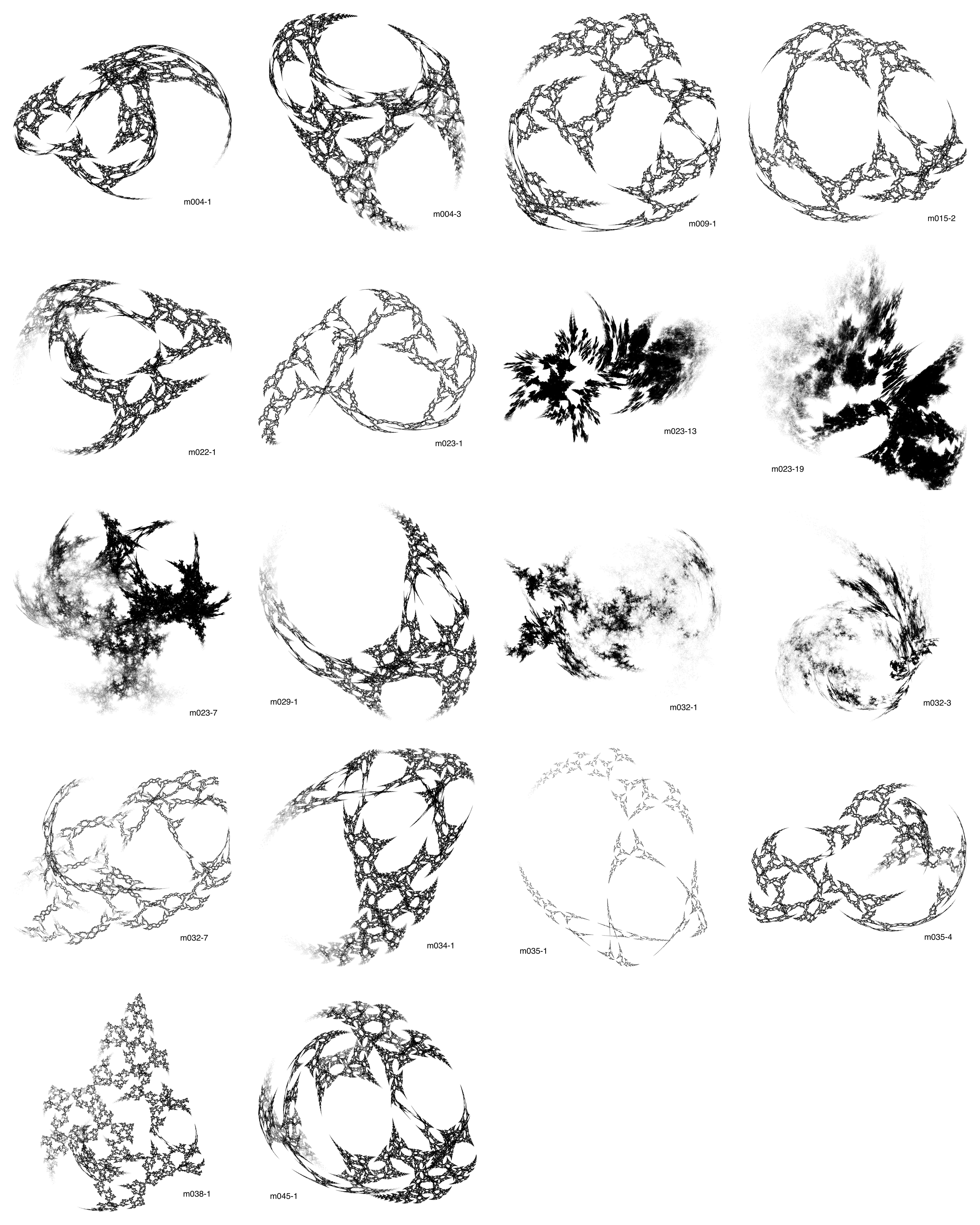
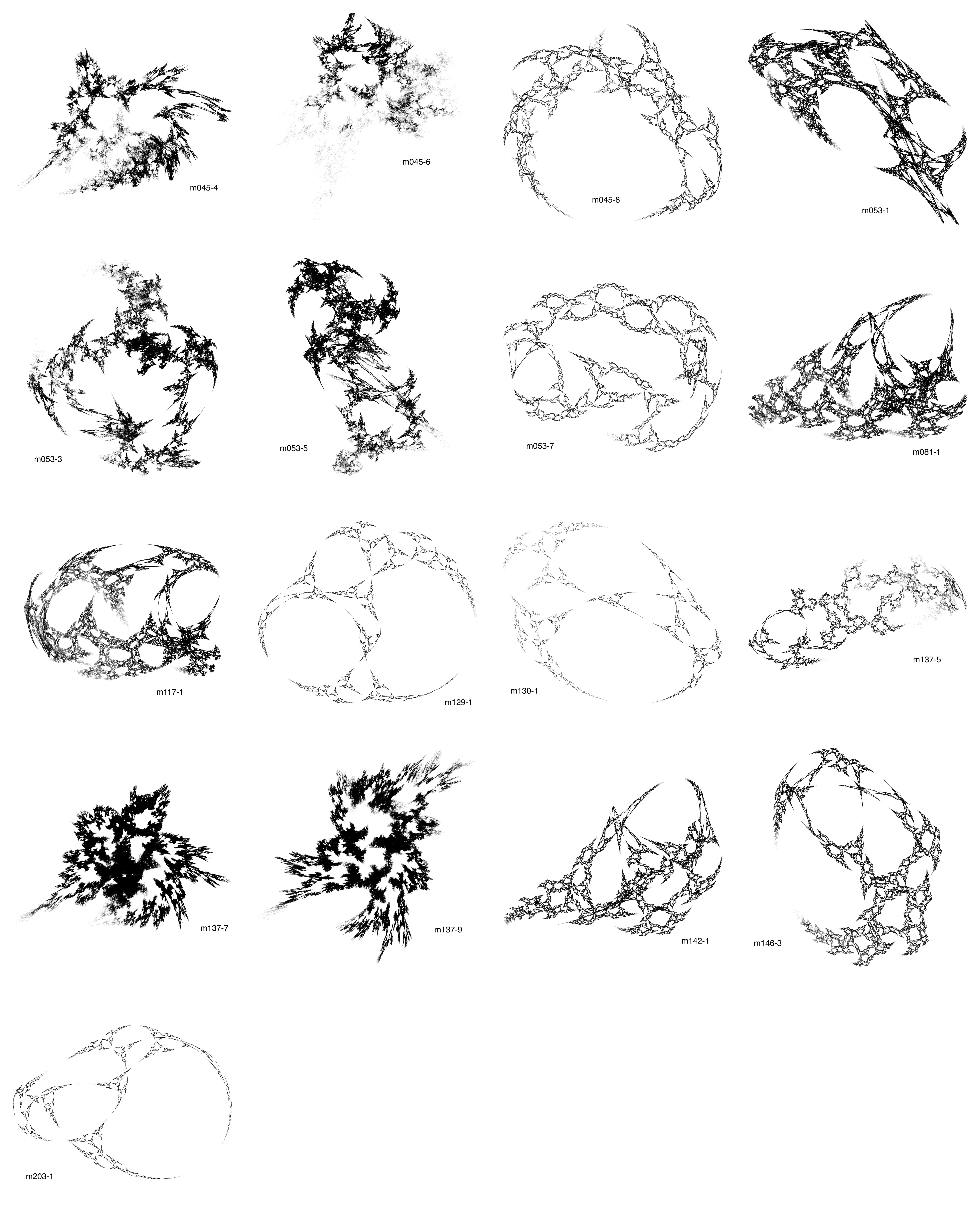
Stored in SnapPy [G“”or] by a joint work of [FKR15] with [GGZ15, GGZ15a], we have at our disposition boundary unipotent representations. By inspection of all the approximated limit sets, we found pairs of representations (paired by complex conjugation in ) that have a fractal limit set.11 1 We also observed that every representation from the census that gave a fractal had each boundary component (a copy of ) sent to a rank one parabolic subgroup. They concern manifolds of the census. In figures 1 and 2 (in the appendix) we exposed all those fractal limit sets.
Among those pairs of representations, are in fact derived from complex hyperbolic triangle groups . They come from manifolds. And among those triangle representations, are derived from complex hyperbolic triangles.
On the remaining pairs, we show that are not surjective morphisms into an index two -triangle group (see proposition 5.2) and that an additional one is a triangular representation, but different from the others (see proposition 5.4): it is a Lagrangian triangle group (as defined in [Wil07]).
We will (mathematically) prove that those triangle representations do in fact come from index two complex hyperbolic triangle groups. All those representations are discrete.
We show that the conjugacy class can be chosen so that generates the boundary holonomy of the fundamental group. This phenomenon is not true in general (see proposition 5.4). For a fixed abstract triangle group, the transformation is unipotent for a unique value of the angular invariant that we will denote .
For each of those triangle representations, we find that the image group is the even-length words subgroup . As it is suggested by its importance, we consider (the abstract version of ) defined by:
| (2) |
The inclusion corresponds to an inclusion morphism defined by and .
Redundancy
We call redundancy the phenomenon of having several manifold fundamental groups represented in a same , or more generally in a same . To assert the equality of the images, we allow conjugacy in and complex conjugation.
Deraux [Der15] first showed that m009 and m015 are two manifolds with representations in a same . But only the representation of m009 is a spherical CR uniformization.
The spherical CR structure is the pair . There is a delicate relationship between a representation of a manifold (of its fundamental group) in and a uniformizable spherical CR representation of . In the latter case, the image group completely determines : if is its discontinuity domain then is diffeomorphic to (that is our definition of being uniformizable, as in [Der15]).
It is very hard in general to determine if a representation in is the holonomy of a spherical CR uniformization. In our study, we relied on [Aco19] to identify uniformizations.
Theorem (4.1).
Consider the following table. Each row consists of manifolds having a boundary unipotent representation with the group denoted in the first column for image (up to conjugation in and complex conjugation).
The manifolds in the column “Uniformization” are (spherical CR) uniformized by their representation and the others in the column “Redundant” are not.
| Group | Uniformization | Redundant |
|---|---|---|
| m004 | m022, m029, m034, m053, m081, m117 | |
| m009 | m015, m035, m142, m146 | |
| m023 | ||
| m039 | m032, m045 | |
| s000 | m053 | |
| m129 | m203 |
Notes
We use the nomenclature of SnapPy for the three-manifolds “mxxx”.
Our proof relies on the computation of a surjective morphism from to . Indeed, we can observe that the data of a surjective morphism into a always furnishes a surjective representation into the corresponding since is always surjective. It will remain to check that the peripheral holonomy is indeed unipotent.
We cannot mathematically prove that the representations appearing in the theorem are the only ones that can be found in the census [G“”or]. There might be other representations in the census that are triangular by a triangle group. But we are strongly confident that we found all of them by the approximation of the limit sets.
A consequence of our work is that the property of having a surjective morphism onto a is not a clearly understood property: some manifolds possess several (e.g. m053) and redundancy frequently occurs.
Deformations
Let have a surjective morphism . Then this (abstract) representation gives various representations . The space of all those representations up to conjugation in has real dimension . The principal invariant to distinguish two representations is the trace of the image of . (See the proposition 4.2 and the following discussion for details.)
The manifolds considered in theorem 4.1 that originally had a few discrete unipotent representations now automatically get a -dimensional subset in their character variety. In general, the character variety has dimension at least two. When it is minimal, as with the figure-eight knot complement, then this construction gives an open component (compare with [Fal+16]).
Numerical approximations of deformations of some triangle groups are available on the webpage of the author [Alea].
In most cases, a surjective morphism is represented in by and gives a boundary unipotent representation of . But this phenomenon is not always true and reveals that complex hyperbolic triangles are not the only ones to be considered.
Proposition (5.4).
There exists a surjective morphism
| (3) |
and a composition having boundary unipotent holonomy. The boundary unipotent representation in is not induced by any representation .
In this case, the boundary holonomy is controlled by the element . (In theorem 4.1 the boundary holonomy is always controlled by .) But for any of representation , the word is never sent to a unipotent element of . This will justify the proposition.
Outline of the paper
In section 2, we succinctly expose a few elements of complex hyperbolic geometry that are needed in the paper. In section 3, we explain how the numerical experiments were driven. We also propose visual clues in order to recognize the limit sets of the various triangle representations . In section 4 we state and show the main result, theorem 4.1. For this, we only employ formal computations, so the result is certain. In section 5 we give other examples. Three examples for which no surjective morphism to does exist. We also show the proposition 5.4, stated earlier.
Methodology
In this paper we deal with two kinds of evidence. What we call experimental arguments are the one arising from the numerical approximations of the limit sets. Those explain how we selected the candidates for triangle representations.
But the results and in particular theorem 4.1 and proposition 5.4 are entirely based on pure mathematical arguments. In fact, they only depend on the description of the fundamental groups of the cited manifolds. Proofs can be checked by hand.
The identification of a representation arising from theorem 4.1 with a corresponding one in the census [G“”or] is made by an exact computation with the formal tools provided by Python and SageMath. The census has its representations stored as matrices with entrees that are polynomial or rational with rational coefficients in an algebraic field. Therefore the representations can be manipulated with exactness. It is only when we numerically approximate the limit sets that we numerically approximate the representations.
We will respect the following rule. The stated theorems, propositions and lemmas are always mathematical. That is to say, proven by hand or by formal (exact) computations.
Note
This paper is part of the author’s thesis, in progress under the supervision of Elisha Falbel.
Acknowledgments
The author enjoyed many and very fruitful conversations. First of all, of course, I am very thankful to Elisha Falbel. Since the early stages in making the experimental tools, Fabrice Rouillier and Antonin Guilloux have been of precious help for the improvement of my code. Across countries, Mathias Görner has been essential to me in order to correctly use the tools provided by SnapPy. I would like to thank Pierre Will for all his comments and the many hours of discussions we had. I have been pleased to exchange with Miguel Acosta about his theorem and about experimental aspects. Finally, I would like to thank the reviewers who gave me many comments significantly improving the text.
2 Elements of complex hyperbolic geometry
In this first section, we expose the main tools and notions in use. One can compare with [Wil16], [Gol99], [Pra05] and [CG74].
We consider the space : it is equipped with the Hermitian product of signature
| (4) |
The subspace of the vectors verifying can be projectivised in and is identified to the complex hyperbolic plane, . In the affine chart , one can identify with the set of vectors verifying . Its boundary in the complex projective plane is a differentiable sphere and is given by . Those points are in correspondance with the non-zero vector lines in verifying .
The unitary group of is and its projectivised version is . The geometrical structure is called the (holomorphic) spherical CR structure.
Let . If has a fixed point in then is elliptic. If with the associated distance function of then is loxodromic (or hyperbolic). Otherwise, is parabolic. One can determine the type of by looking at its trace. We follow Goldman [Gol99] and let
| (5) |
If then is loxodromic, if then is elliptic (in fact regular elliptic: all its eigenvalues are different).
When there are three cases: if then is (parabolic) unipotent (all its eigenvalues are ), otherwise it is either elliptic (and therefore a reflection with respect to a point or a complex geodesic) or ellipto-parabolic (a screw transformation along a complex geodesic). Note that when is real:
| (6) |
and (under the hypothesis that is real) is therefore regular elliptic if , is loxodromic if and is unipotent if . Note that unipotent transformations are a special kind of parabolic elements.
Let be a smooth manifold and its fundamental group. A representation is the holonomy of a (CR) uniformization of if, with the domain of discontinuity of , the quotient (that is generally only an orbifold) is a manifold diffeomorphic to . When is discrete, , where is the limit set of . The next section will describe this set. A manifold admitting such a representation is said to be (CR) uniformizable. Those manifolds are central in the study of spherical CR structures and are determined by the algebraic data of . In general, even when is a smooth manifold, it is too hard to identify it. It remains unknown which three-manifolds are CR uniformizable.
2.1 Limit sets
Let be a subgroup. Its limit set is given by:
| (7) |
where is any point ( is independent of this choice) and where the overline denotes the topological closure in .
Lemma 2.1.
The main properties of this set are the following. (Compare with [CG74].)
- 1.
The limit set is compact and -invariant.
- 2.
If is compact, -invariant and is constituted of at least two points, then .
- 3.
If then fixes a point in .
- 4.
If has at most two points, then (or ) is said to be elementary, otherwise it has an infinite number of points and is perfect (each point is an accumulation point).
An important result is the following.
Proposition ([CG74]).
If is not discrete then is either elementary, or equal to , or equal to the boundary of a totally geodesic proper subspace, that is to say a smooth circle.
By consequence, if is a fractal (none of the above cases), then is discrete. It is a powerful experimental way to investigate if is discrete. Note that there is no general mathematical procedure to prove with certainty that a subgroup is discrete or not.
The self-similarity property of limit sets can be justified by the following lemma.
Lemma 2.2.
Let be a discrete subgroup of and suppose that is not elementary. Let be any point and be any open neighborhood of . Then there exists such that
| (8) |
Proof.
Let . It is compact and -invariant. By construction, cannot have more than one point. If then fixes and must be elementary since it is discrete. Therefore and it follows that . By compactness of , only a finite number of are necessary. ∎
2.2 Complex hyperbolic triangle groups
We will now describe more precisely the complex hyperbolic triangle groups
| (9) |
with , and all three being complex reflections. The numbers are integers possibly infinite. If one of those is infinite, then the corresponding relation is omitted.
We will prove that only depends on and an additional real parameter , up to conjugation and complex conjugation. This parameter will be determined by the value of the trace of . In particular, for any triplet , we obtain a unique complex hyperbolic triangle group, up to conjugation and complex conjugation, with unipotent. This will justify the notation to identify a complex hyperbolic triangle group.
Recall from the introduction that we can see a complex hyperbolic triangle group as a representation in by complex reflection of the abstract triangle group
| (10) |
When complex hyperbolic triangle groups were exposed by Schwartz [Sch02], he asked the following: when is a complex hyperbolic triangle group a discrete and injective representation of the corresponding abstract triangle group? He proposed the following important conjecture.
Conjecture 2.3 (Schwartz).
A complex hyperbolic triangle group is a discrete and injective representation of in , if and only if and are both not elliptic.
Note that, in some rare cases, can remain discrete (but not injective) with and elliptic of finite order. For example, Thompson [Tho10] found a representation with of order and a representation with of order , and both representations are lattices of .
Schwartz [Sch07] has shown his conjecture when is large enough. A first step toward the general case is a result due to Grossi [Gro07]. In particular for , Grossi shows that if is not elliptic then is not either. A proof of Schwartz’ conjecture in the case of has been given by Parker, Wang and Xie [PWX16] and the case of has been studied by Parker and Will [PW17].
Theorem 2.4 ([PWX16],[PW17]).
Let . Let be a hyperbolic triangle group. Then is discrete and faithful if and only if is not elliptic.
Now we proceed to a description of complex hyperbolic triangle groups. Let be a complex hyperbolic triangle group, with and . Each reflection fixes a complex line (isomorphic to ) in . Let , and be the vector hyperplanes of covering those complex lines.
Let , and be the dual complex lines of those hyperplanes defined by . The group is fully described by them. Since is a complex line of , it is a negative-type complex plane of (), and is a positive-type complex line of ().
We only need to choose a basis vector for each in order to describe those lines. We say that the triangle group is non-degenerate when such basis vectors form a basis of . We will make this assumption from now on.
Let be a basis vector of , then
| (11) |
is a complex reflection and verifies for any . That is to say, in , . Therefore indeed defines the reflection fixing . Because , one can normalize so that .
The last free parameters describing the ’s are an angle for each . One can set and then modify and so that and are real and positive. In general, is not real and this lack can be measured by . From an intrinsic point of view, that is to say without choosing the ’s, the default for the vertices to be in a same real plane can be measured by
| (12) |
The value of is also known under the name of the angular invariant.
Once are known, it is easy to evaluate the matrices of , and in the basis .
| (13) | ||||
| (14) | ||||
| (15) |
We still have to see how , , and determine . For the time being, we suppose . In fact, we will prove that the matrix given by the ’s is equal to:
| (16) |
And this shows that the ’s fully determine , , and in return. This matrix is an Hermitian form preserved by , and . The determinant of this matrix is given by
| (17) |
This determinant allows us to decide when has for signature. Since the trace of is , it implies that at least one eigenvalue is positive. Therefore, its determinant is negative if and only if has for signature. That is equivalent to:
| (18) |
That must be the case since the original Hermitian form has for signature.
If then vanishes and one can make both and real. Therefore, complex hyperbolic triangle groups are rigid: is always zero.
We now justify the expression of by computing the ’s. Up to conjugation, we can suppose that is generated by . This implies that and are both of the form . Therefore, every is given by since at least one of or has a vanishing third coordinate.
Therefore, geometrically speaking, is the cosine of the angle in formed by the complex lines generated by the first two coordinates of and . It is the real part of that is equal to the cosine of the angle formed by the vectors given by the first two coordinates of and (see [Gol99, p. 36]). In other terms, if is real and are unitary then with . If additionally then (that will be the case for us).
Note that is non real in general, but of course is real and can even be assumed to be positive. The angle formed by and is equal to since . By taking the duals and , we get . Likewise, and .
Finally, one can compute, with :
| (19) |
and note that in our conventions, we have . It shows that determines once is known. Since the complex conjugation changes into , we deduce from our discussion the following results. In the case where we have in fact:
| (20) |
Proposition ([Pra05]).
Let be such that . A representation of the triangle group
| (21) |
into is determined by up to conjugation, with as previously. Up to conjugation and complex conjugation, it is determined by , with pairwise distinct.
Furthermore, verifies
| (22) |
and conversely, this condition suffices to define a representation with that value of .
The parameter can be taken in since the complex conjugation exchanges and . The possible values of are constrained by the preceding condition. For example, when , we have
| (23) |
If we take a look at the trace of , its maximum is given for minimal (that is to say ) and its minimum by the maximum of . We have the inequalities:
| (24) | ||||
| (25) |
This computation shows that the range of the values of is included in and therefore, the range for which is discrete is of the form , with the maximum stated before. The value is indeed reachable: the minimum value for is , since we have to verify , and the maximum value of is indeed reached when is minimal. This value for is .
One can compute the angular invariant required to have unipotent. It is given by:
| (26) |
When one or several of , and are non finite, we can get similar results by replacing the undefined with , where is the distance between the two complex hyperbolic geodesics and . See [Pra05]. In particular, it is still true that is determined by .
3 Experimental approach
In this section, we explain how we approximate the limit sets of the representations appearing in the census [G“”or].
We also propose a comparative experiment by simulating the limit sets associated to the triangle groups. Since, up to conjugation and complex conjugation, there is a unique with unipotent, the limit set is itself unique up to translation and complex conjugation.
It will allow us to propose visual clues in order to distinguish the different triangle group fractals when is unipotent.
The source code of the simulations and most of their results are available on the author’s webpage [Alea]. The code has been made open-source [Ale].
3.1 Computing limit sets
Lemma 3.1.
Let be a subgroup. Let denote the subset of the loxodromic elements. Suppose . Then the closure of the accumulation points for the iteration dynamic:
| (27) |
is equal to the full limit set .
Proof.
Note that if is loxodromic then after any conjugation, is again loxodromic.
The set is compact and has at least two points. By definition, . So we only need to show that is -invariant, implying .
For any , we have . But is loxodromic and its only attractive fixed point is the limit point for the orbits from both and . Therefore which shows the -invariance. It implies by minimality of . ∎
This lemma suggests a strategy to approximate : compute the attractive limit points of the loxodromic elements of . However, this strategy requires to compute a very large number of elements . This can be done by generating words of length . If is described by two generators, then there are approximately words of length .
In practice, and this is particularly true with complex hyperbolic triangle groups, it is hard to get different points from such a computation. One can often see large concentrations of points in tiny boxes and even many copies of the same point. This is partly due to unknown relations between words, even at small length words.
Instead of only computing words and getting their attractive limits, we used a second strategy in complement. When enough points are acquired, one can apply words on them (loxodromic or not) to get a better picture of the limit set. This method is much more efficient for it rarely makes redundant images. When nice symmetries are known (and for example, with complex hyperbolic triangles one knows the reflections , and ), this allows a much better result.
In practice, we first compute the attractive points of -length words, then apply given symmetries on the set obtained, then apply -length words on them, and apply again symmetries.
3.2 Complex hyperbolic triangle groups
To compute the limit sets associated to -representations of triangle groups, we used our previous parametrization of the complex reflections , , and . We picked the angular invariant for which is unipotent.
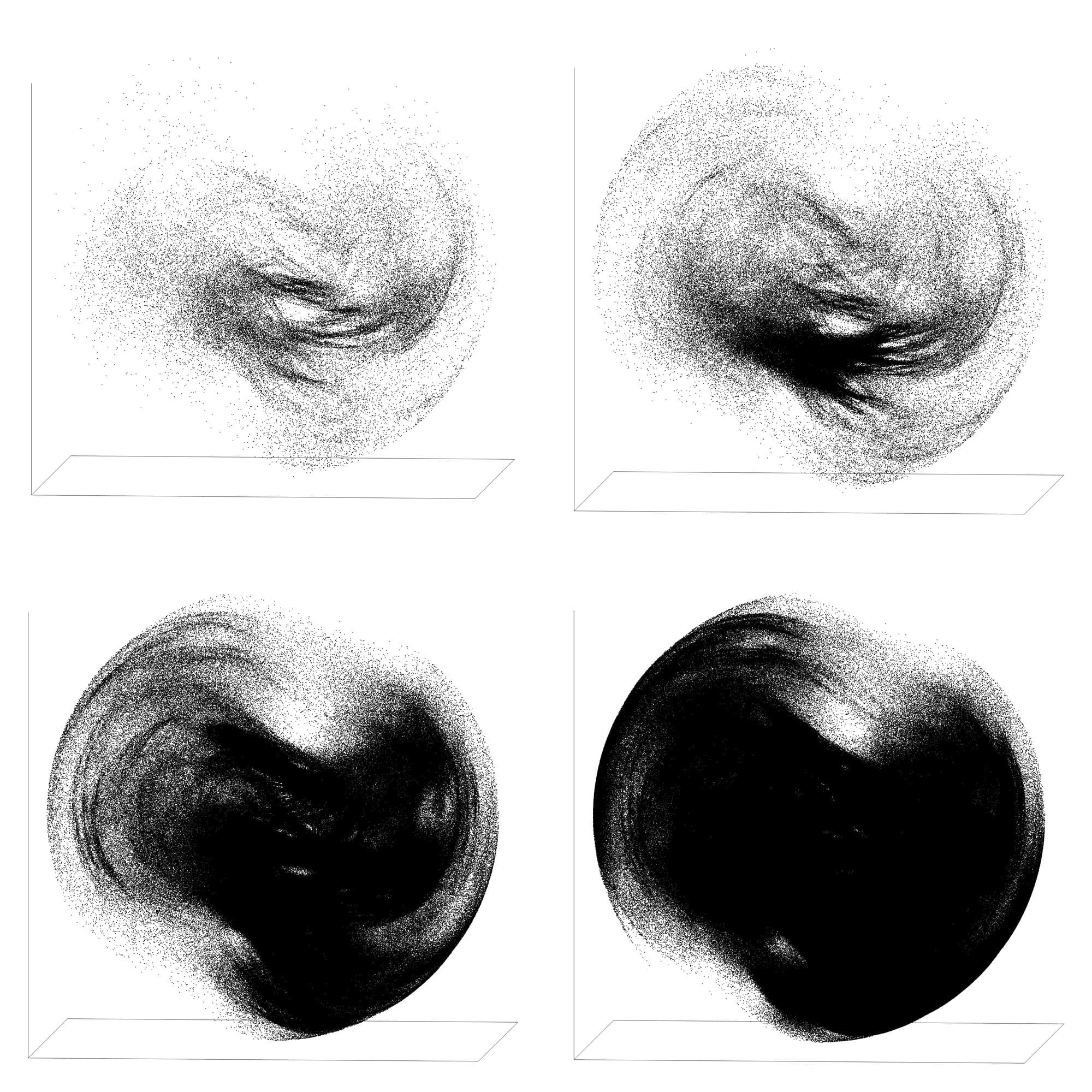
For we show three projections of the limit set and an additional diagram proposing a visual clue to recognize the limit set, see figures 5, 6, 7, and 8 in the appendix. This visual clue consists in looking for a pair of symmetric spikes and inspect the middle. We count the largest outer holes. When there is none, when there is one, when there are two, when there are three, etc.
4 Morphisms and redundancy
From the census of the boundary unipotent representations in [FKR15] and stored in SnapPy [G“”or], we numerically approximated all their limit sets. After a visual inspection, we kept the representations that gave fractals (see [Alea] for the numerical results and the figures 1 and 2).
Those representations come in pairs by complex conjugation of the coefficients. In this section, we study many of them by a classification into triangle groups. pairs will be directly classified and more will be constructed. The classification will be systematic, following a method that we will describe.
Notes on the selection
It is already known that m004-1 and m004-3 are related by the composition of a figure-eight knot’s symmetry (see [DF15]). Therefore we only classify one of the two with the systematic procedure.
A representation of m038 presents the characteristics of a complex hyperbolic triangle group. Indeed, m038 has such a representation according to a preprint of Ma and Xie [MX20] that the author has been able to consult. A representation of m137 presents the characteristics of a complex hyperbolic triangle group.
We summarize the mathematical result in the following theorem. It is fully independent from the numerical computations. The method of the proof will be explained later.
Recall that denotes the even-length subgroup of , where the angular invariant is chosen so that is unipotent.
Theorem 4.1.
Consider the following table. Each row consists of manifolds having a boundary unipotent representation with the group denoted in the first column for image (up to conjugation in and complex conjugation).
The manifolds in the column “Uniformization” are (spherical CR) uniformized by their representation and the others in the column “Redundant” are not.
| Group | Uniformization | Redundant |
|---|---|---|
| m004 | m022, m029, m034, m053, m081, m117 | |
| m009 | m015, m035, m142, m146 | |
| m023 | ||
| m039 | m032, m045 | |
| s000 | m053 | |
| m129 | m203 |
The manifolds m039 and s000 do not appear in the census of [FKR15] for there are respectively described by five and six tetrahedra. But the result still applies and we will construct their triangular representations with boundary unipotent holonomy from their fundamental groups. We found those manifolds by applying the theorem of Acosta (see below).
The manifold m053 will be treated differently than the other members of the census. The initial description in SnapPy of its two triangular representations m053-1 and m053-7 are quite hard to use. We proceed the computation of another description (with the help of the method Manifold.randomize() of SnapPy).
Note that for each row, at most one representation is a uniformization of the corresponding manifold. Deraux [Der15] encountered the same phenomenon with the manifolds m009 and m015. In fact, we identify the uniformizations with the following result of Acosta.
Theorem ([Aco19]).
Let . The manifold at infinity of is the Dehn filling with slope of any cusp of the Whitehead link complement.
With SnapPy, it is possible to compute Dehn surgeries on the Whitehead link complement. Note that m129 is the Whitehead link complement in our table. One has to be careful: the marking of the peripheral holonomy is not unique, with SnapPy one needs to call the manifold and fill a cusp with the meridian equal to and the longitude equal to .
This procedure gives the selection of the uniformized manifold along each row. Note that we do have a true CR uniformization since Acosta did construct the CR structures by CR surgery. (It is not only a topological result.)
The first uniformization of m129 (the Whitehead link complement) was shown by Schwartz [Sch01], but the present uniformization by a triangle group with boundary unipotent holonomy was studied by Parker and Will [PW17].
We now explain how we prove the rest of theorem 4.1. We start with the following fundamental result about subgroups generated by two elements. It is the restricted case of a more general result in .
Proposition 4.2 ([Law07, Wil09]).
If is a group generated by two elements and , then any irreducible representation is fully determined up to conjugation in by and .
In fact, in , is a root of a second degree polynomial with real coefficients and the two roots are either equal or complex conjugates.
With
| (28) |
recall that we have a surjective morphism given by . The traces of the images of and are all real and prescribed by the data . (When , we send to a unipotent transformation.) Therefore, by doing a complex conjugation on the representation, we only conjugate the trace of the image of .
Corollary 4.3.
Let be a fundamental group generated by two elements and . Let be a representation. Let be a surjective morphism and be the composition of with .
Let be such that and , . We make the following hypotheses:
- 1.
The traces and coincide on the words and .
- 2.
There exists such that , and , .
Then and are equal up to conjugation and complex conjugation.
Proof.
Given the notations, the first assumption shows that and are equal up to complex conjugation and conjugation on .
Up to the conjugations, assume that on . Then by the second hypothesis and . Therefore, on . ∎
Recall that the trace of a transformation determines its type. If a transformation is elliptic with order , then . The transformation is unipotent if, and only if, and .
The method
This is how we will identify all our boundary unipotent representations. An application of this method is detailed in the next section.
- 1.
We describe the relation of as consequence of several simpler relations “of triangle type”. Those simpler relations are verified by the representation in the census (but not by ).
For example, is implied by , and . It is the most challenging step and also the most important. It is in general very difficult to find such simpler relations.
This step is inscribed in the first table. The “id” column allows us to recover the representation from SnapPy. Relations can be checked with the SageMath code in the appendix.
- 2.
We construct the surjective morphism and recover the values of the various words and . We use the previous relations “of triangle type” to check that we have a morphism. This step is inscribed in the second and third tables. It is a completely autonomous step from all the computations. It only involves and by hand computations.
- 3.
We find values of and and it can be checked by hand that they verify the required equalities for both and . Those words are inscribed in the third table.
- 4.
We verify that the traces of the four elements match with the evidence of the first step and by exact computations, e.g. for (see the SageMath code in the appendix for this).
Those four steps prove the identification we are looking for. But we add a last table with the description of the peripheral holonomy. The reason is that one can only consider the second step (doable by hand) and with the last table show that the morphism constructed has boundary unipotent holonomy, independently from the census. (One should play with various the conjugations such as and in .)
For the construction of this last table, we only use the relations described in the first step and implied by the description of the morphism.
Proof of theorem 4.1.
Let be a manifold in the table and an assigned group. By the second step, we construct a morphism . This morphism gives a representation by the composition . Finally, has boundary unipotent holonomy by the last table. ∎
On the notations
We keep the notations of the corollary and write instead of respectively.
4.1 – m004, m022, m029, m034, m081 and m117
We survey the method for m004-1. We denote this representation by . By SnapPy, the fundamental group of m004 is presented by the generators and and the relation .
In the census, is a representation verifying (by exact computation) the relations , and . Those three relations alone imply the one of the fundamental group: .
Those first datas are reported in the first table. They suggest that we should seek for a triangle group representation.
We define a new morphism by and . To check that this is indeed a morphism, it suffices to check the relations . And that is the case: in , has order , has order and is sent on that has order since has order . This is given in the second table.
With the data of the third table, we show that we have constructed a surjective morphism . Since is generated by and , it suffices to give antecedents to both. The word in is sent to and the word is sent to .
Now we prove that (which is the composition of with ) and have equal images up to conjugation and complex conjugation. According to corollary 4.3, it suffices to find the words and . This is all given in the third table and verifications are straightforward.
The traces of will coincide since they verify the triangular relations in both representation and . With the word we check by formal computation that the trace under is indeed .
If one does not want to involve the representation of the census, but only construct the morphism a priori, the last table allows us to check that the boundary is unipotent under composed with the usual map . Here, the boundary is described by the two words and . Under , we have and that is indeed mapped to a unipotent element of .
| id | relation | Relations | |
|---|---|---|---|
| m004-1 | [0,0] | , , | |
| m022-1 | [0,0] | , , | |
| m029-1 | [0,0] | , , | |
| m034-1 | [0,0] | , , | |
| m081-1 | [0,0] | , , | |
| m117-1 | [0,0] | , |
| m004 | ||
|---|---|---|
| m022 | ||
| m029 | ||
| m034 | ||
| m081 | ||
| m117 |
| m004 | ||||||
| m022 | ||||||
| m029 | ||||||
| m034 | ||||||
| m081 | ||||||
| m117 |
| Peripheral | holonomy | |
|---|---|---|
| m004 | ||
| m022 | ||
| m029 | ||
| m034 | ||
| m081 | ||
| m117 |
4.2 – m009, m015, m035, m142 and m146
| id | relation | Relations | |
|---|---|---|---|
| m009-1 | [0,1] | , , | |
| m015-2 | [0,1] | , , | |
| m035-5 | [0,3] | , , | |
| m142-1 | [0,0] | , , | |
| m146-3 | [0,3] | , , |
| m009 | ||
|---|---|---|
| m015 | ||
| m035 | ||
| m142 | ||
| m146 |
| m009 | ||||||
| m015 | ||||||
| m035 | ||||||
| m142 | ||||||
| m146 |
| Peripheral | holonomy | |
|---|---|---|
| m009 | ||
| m015 | ||
| m035 | ||
| m142 | ||
| m146 |
4.3 – m023
| id | relation | Relations | |
|---|---|---|---|
| m023-1 | [0,0] | , , |
| m023 |
|---|
| m023 |
| Peripheral | holonomy | |
|---|---|---|
| m023 |
4.4 – m032 and m045
| id | relation | Relations | |
|---|---|---|---|
| m032-7 | [0,2] | , , | |
| m045-8 | [0,4] | , , |
| m032 | ||
|---|---|---|
| m045 |
| m032 | ||||||
| m045 |
| Peripheral | holonomy | |
|---|---|---|
| m032 | ||
| m045 |
4.5 – m129 and m203
With the complex hyperbolic triangle group we ask to be unipotent: we send to a unipotent transformation.
| id | relation | Relations | |
|---|---|---|---|
| m129-1 | [0,0] | , | |
| m203-1 | [0,0] | , |
| m129 | ||
|---|---|---|
| m203 |
| m129 | ||||||
| m203 |
| Peripheral | holonomy | |
|---|---|---|
| m129 | ||
| m203 | ||
4.6 m039, s000 and m053
In this final section, we construct the remaining representations with boundary unipotent holonomy. We were not able to identify them with representations from the census for the following reasons.
For m039 and s000 this comes from the fact that they are described by respectively five and six tetrahedra and therefore are not part of the census. For m053, the initial description provided is too complicated to be used out of the box. But with an other description, one can still give triangular representations and the identification with m053-1 and m053-7 follows from the visual clues.
For those representations, we follow the same method to construct the representations, with the exception of the experimental verification of the traces and relations that are not necessary here.
| relation | Relations | |
|---|---|---|
| m039 | , , | |
| m053 | , , | |
| , , | ||
| s000 | , , |
| Triangle | |||
|---|---|---|---|
| m039 | |||
| m053 | |||
| m053 | |||
| s000 |
| Triangle | |||||
|---|---|---|---|---|---|
| m039 | |||||
| m053 | |||||
| m053 | |||||
| s000 |
| Peripheral | holonomy | |
|---|---|---|
| m039 | ||
| m053 | ||
| with | ||
| with | ||
| s000 |
5 More diverse examples
To study more examples, we note the following. Let be a hyperbolic manifold with one cusp. If a representation has for boundary a parabolic subgroup of rank one (generated by a single element), then there exists a relation between the two generators of its peripheral holonomy. This relation can be used to factorize the morphism through a Dehn filling.
Now, a manifold on which we executed a Dehn filling will have a different presentation. Often, this presentation enables to see more rapidly the triangle group involved if we are in the case of theorem 4.1.
5.1 A homological obstruction
The existence of a surjective morphism (as in theorem 4.1) is submitted to an easy criterium.
Lemma 5.1.
If there exists a surjective morphism then there exists a surjective morphism , where we took the abelianizations.∎
Among the representations not covered in theorem 4.1, there are three that have a fractal limit set corresponding to a .
The representation m045-1 shows the sign of a group as image. See its approximated limit set (figure 11) and compare with the visual clues (figure 5) in the appendix.
The representations m035-1 and m130-1 both resemble to . Compare figures 9 and 10. See also [Alea] for the numerical approximations in a three-dimensional display.
Proposition 5.2.
The boundary unipotent representations m045-1, m035-1 and m130-1 do not verify theorem 4.1. That is to say, those representations are not surjective morphisms of the form .
In the case of , the abelianization of this abstract group is or depending on the class of modulo . For we get , and for we get .
Proof of proposition 5.2.
The representation m045-1 (with id [0,0]) has boundary unipotent holonomy of rank one. Therefore, with a relation between the two peripheral curves.
This relation gives a factorization by the corresponding Dehn filling. In fact, in the terms of SnapPy and the data of m045-1 in [G“”or], we get the Dehn filling . This can be verified with exact computations with the code in the appendix.
Computations of SnapPy show . But and are relatively prime and therefore there exists no surjective morphism from to , giving an impossibility with the previous lemma.
Similarly, the representations m035-1 (of id [0,0]) and m130-1 (of id [0,1]) factorize through the Dehn fillings and respectively.
Now, and . Thus there can’t be any surjective morphism to , raising an impossibility with the lemma. ∎
The fact that m045-1 has a limit set so similar to the one of suggests the existence of a close relationship. For instance, there might exist a morphism with finite index image in . But this remains an open question.
5.2 A Lagrangian triangle group
As we will see (proposition 5.4), there exists at least one representation with boundary unipotent holonomy,
| (29) |
surjective on but that cannot be factorized by
| (30) |
Lemma 5.3.
For any , let be a representation with unipotent. Then is not real.
Proof.
We use the exact parametrization of Guilloux and Will [GW19]. The formal computations that we will described have too many terms to be reproduced here, but they can be recovered in the code of the author [Ale] or directly reproduced with the description of [GW19].
Recall with proposition 4.2 that the discriminant of the equation for which is solution is always negative or null. Since we want , we must have . This equation can be solved by exact computations and is only a function of since and are determined by their elliptical order.
With the resolution of in terms of the only free variable , one can compute explicitly and solve the equation in terms of . It is again a quadratic equation. There are in general two solutions and are complex conjugates. We take the solution with positive imaginary part.
Numerical approximations show that for any , the imaginary part of is always non zero. For example, when , . ∎
The representation m023-7 (with id [0,4]) of the census has a limit set different from the usual triangular subgroups, see figure 12. The boundary holonomy has rank one, and therefore m023-7 factorizes through a Dehn filling. In this case, it is .
Proposition 5.4.
There exists a surjective morphism
| (31) |
and a composition having boundary unipotent holonomy. The boundary unipotent representation in is not induced by any representation .
Note that any inclusion sends to a matrix with real trace in . Indeed, when described in terms of and , we have and this is the product of two reflections.
Proof.
One of the presentations of given by SnapPy (using also M.randomize()) is
| (32) |
with the peripheral curves given by and . Now, we define
| (33) |
and one can verify the relations of the fundamental group but also .
The boundary holonomy of this representation is prescribed by and this word has for image . We conclude with the previous lemma. ∎
Now we can compare the fractal of m023-7 with the one of sending to a unipotent element as in the lemma (figure 13). Visually, they match indeed.
Denote the surjective morphism from the proposition. Denote its composition with sending to a unipotent element.
A consequence of the fact that is that is -decomposable: it is generated by three antiholomorphic reflections. This comes from a theorem of Paupert and Will:
Theorem.
[PW17a] Let be two isometries not fixing a common point in . Then the pair is -decomposable if and only if the commutator has a fixed point in whose associated eigenvalue is real and positive.
6 Appendix: figures and code



References
- [Aco19] Miguel Acosta “Spherical CR uniformization of Dehn surgeries of the Whitehead link complement” In Geom. Topol. 23.5, 2019, pp. 2593–2664 DOI: 10.2140/gt.2019.23.2593
- [Ale] R.. Alexandre “https://github.com/R-Alexandre/CRLimitSets”
- [Alea] R.. Alexandre “https://rphalexandre.fr/ensembles-limites/”
- [CG74] Shyan. Chen and Leon Greenberg “Hyperbolic spaces” In Contributions to analysis (a collection of papers dedicated to Lipman Bers), 1974, pp. 49–87
- [Der15] Martin Deraux “On spherical CR uniformization of 3-manifolds” In Exp. Math. 24.3, 2015, pp. 355–370 DOI: 10.1080/10586458.2014.996835
- [DF15] Martin Deraux and Elisha Falbel “Complex hyperbolic geometry of the figure-eight knot” In Geom. Topol. 19.1, 2015, pp. 237–293 DOI: 10.2140/gt.2015.19.237
- [Fal08] Elisha Falbel “A spherical CR structure on the complement of the figure eight knot with discrete holonomy” In J. Differential Geom. 79.1, 2008, pp. 69–110
- [Fal+16] E. Falbel et al. “Character varieties for : the figure eight knot” In Exp. Math. 25.2, 2016, pp. 219–235 DOI: 10.1080/10586458.2015.1068249
- [FK00] Elisha Falbel and Pierre-Vincent Koseleff “Flexibility of ideal triangle groups in complex hyperbolic geometry” In Topology 39.6, 2000, pp. 1209–1223 DOI: 10.1016/S0040-9383(99)00023-3
- [FKR15] Elisha Falbel, Pierre-Vincent Koseleff and Fabrice Rouillier “Representations of fundamental groups of 3-manifolds into : exact computations in low complexity” In Geom. Dedicata 177, 2015, pp. 229–255 DOI: 10.1007/s10711-014-9987-x
- [GGZ15] Stavros Garoufalidis, Matthias Goerner and Christian. Zickert “Gluing equations for -representations of 3-manifolds” In Algebr. Geom. Topol. 15.1, 2015, pp. 565–622 DOI: 10.2140/agt.2015.15.565
- [GGZ15a] Stavros Garoufalidis, Matthias Goerner and Christian. Zickert “The Ptolemy field of 3-manifold representations” In Algebr. Geom. Topol. 15.1, 2015, pp. 371–397 DOI: 10.2140/agt.2015.15.371
- [Gol99] William. Goldman “Complex hyperbolic geometry”, Oxford Mathematical Monographs The Clarendon Press, Oxford University Press, New York, 1999
- [G“”or] Mathias G“”orner “http://ptolemy.unhyperbolic.org”
- [Gro07] Carlos. Grossi “On the type of triangle groups” In Geom. Dedicata 130, 2007, pp. 137–148 DOI: 10.1007/s10711-007-9209-x
- [GW19] Antonin Guilloux and Pierre Will “On -representations of the Whitehead link group” In Geom. Dedicata 202, 2019, pp. 81–101 DOI: 10.1007/s10711-018-0404-8
- [Law07] Sean Lawton “Generators, relations and symmetries in pairs of unimodular matrices” In J. Algebra 313.2, 2007, pp. 782–801 DOI: 10.1016/j.jalgebra.2007.01.003
- [MX20] Jiming Ma and Baohua Xie “Three-manifolds at infinity of complex hyperbolic orbifolds” Preprint, 2020
- [Pra05] Anna Pratoussevitch “Traces in complex hyperbolic triangle groups” In Geom. Dedicata 111, 2005, pp. 159–185 DOI: 10.1007/s10711-004-1493-0
- [PW17] John. Parker and Pierre Will “A complex hyperbolic Riley slice” In Geom. Topol. 21.6, 2017, pp. 3391–3451 DOI: 10.2140/gt.2017.21.3391
- [PW17a] Julien Paupert and Pierre Will “Real reflections, commutators, and cross-ratios in complex hyperbolic space” In Groups Geom. Dyn. 11.1, 2017, pp. 311–352 DOI: 10.4171/GGD/398
- [PWX16] John. Parker, Jieyan Wang and Baohua Xie “Complex hyperbolic triangle groups” In Pacific J. Math. 280.2, 2016, pp. 433–453 DOI: 10.2140/pjm.2016.280.433
- [Sch01] Richard Schwartz “Degenerating the complex hyperbolic ideal triangle groups” In Acta Math. 186.1, 2001, pp. 105–154 DOI: 10.1007/BF02392717
- [Sch02] Richard Schwartz “Complex hyperbolic triangle groups” In Proceedings of the International Congress of Mathematicians, Vol. II (Beijing, 2002) Higher Ed. Press, Beijing, 2002, pp. 339–349
- [Sch07] Richard Schwartz “Spherical CR geometry and Dehn surgery” 165, Annals of Mathematics Studies Princeton University Press, Princeton, NJ, 2007
- [Tho10] James. Thompson “Complex hyperbolic triangle groups”, 2010
- [Wil07] Pierre Will “The punctured torus and Lagrangian triangle groups in ” In J. Reine Angew. Math. 602, 2007, pp. 95–121 DOI: 10.1515/CRELLE.2007.004
- [Wil09] Pierre Will “Traces, cross-ratios and 2-generator subgroups of ” In Canad. J. Math. 61.6, 2009, pp. 1407–1436 DOI: 10.4153/CJM-2009-067-6
- [Wil16] Pierre Will “Two-generator groups acting on the complex hyperbolic plane” In Handbook of Teichmüller theory. Vol. VI 27, IRMA Lect. Math. Theor. Phys. Eur. Math. Soc., Zürich, 2016, pp. 275–334
- [Wil21] Pierre Will “Autour de la géométrie hyperbolique complexe : , et quelques 3-variétés” Habilitation à diriger des recherches, 2021