A Two-Stage Bayesian Semiparametric Model for Novelty Detection with Robust Prior Informationhttps://doi.org/10.1007/s11222-021-10017-7
Abstract
Novelty detection methods aim at partitioning the test units into already observed and previously unseen patterns. However, two significant issues arise: there may be considerable interest in identifying specific structures within the novelty, and contamination in the known classes could completely blur the actual separation between manifest and new groups. Motivated by these problems, we propose a two-stage Bayesian semiparametric novelty detector, building upon prior information robustly extracted from a set of complete learning units. We devise a general-purpose multivariate methodology that we also extend to handle functional data objects. We provide insights on the model behavior by investigating the theoretical properties of the associated semiparametric prior. From the computational point of view, we propose a suitable -sequence to construct an independent slice-efficient sampler that takes into account the difference between manifest and novelty components. We showcase our model performance through an extensive simulation study and applications on both multivariate and functional datasets, in which diverse and distinctive unknown patterns are discovered.
Keywords: Bayesian mixture model, Bayesian nonparametrics, Minimum Regularized Covariance Determinant, Novelty detection, Slice sampler.
1 Introduction
Supervised classification techniques aim at predicting a qualitative output for a test set by learning a classifier on a fully-labeled training set. To this extent, classical methods assume that the labeled units are realizations from each and every sub-groups in the target population. However, many real datasets contradict these assumptions. As an example, one may think about an evolving ecosystem in which novel species are likely to appear over time. In other words, basic classifiers cannot handle the presence of previously unobserved - or hidden - classes in the test set. Novelty detection methods, also known as adaptive methods, address this issue by modeling the presence of classes in the test set that have not been previously observed in the training. Relevant examples of this type of data analysis include, but are not limited to, radar target detection (Carpenter et al. 1997), detection of masses in mammograms (Tarassenko et al. 1995), handwritten digit recognition (Tax & Duin 1998) and e-commerce (Manikopoulos & Papavassiliou 2002), for which labeled observations may not be available for every group.
Within the model-based family of classifiers, adaptive methods recently appeared in the literature. Miller & Browning 2003 pioneer a mixture model methodology for class discovery. Bouveyron 2014 introduces an adaptive classifier in which two algorithms, based respectively on transductive and inductive learning, are devised for inference. More recently, Fop et al. 2021 extend the original work of Bouveyron 2014 by accounting for unobserved classes and extra variables in high-dimensional discriminant analysis.
Classical model-based classifiers are not robust, as they lack the capability of handling outlying observations in the training and in the test set. On the one hand, the presence of outliers in the training set can significantly alter the learning phase, resulting in poorly representative classes and therefore jeopardizing the entire classification process. In the training set, we identify as outliers units with implausible labels and/or values. Cappozzo et al. 2020 extend the work of Bouveyron 2014 addressing this problem by using a robust estimator that relies on impartial trimming (Gordaliza 1991). In short, the most unlikely data points under the currently estimated model are discarded. On the other hand, dealing with outliers in the test set is a more delicate task. Ideally, we would like to distinguish between novelties, i.e., test observations displaying a common, specific pattern, and anomalies, i.e., test observations that can be regarded as noise. While the distinction between novel and anomalous entities is most often apparent in practice, there exist some circumstances under which such separation is vague and somewhat philosophical. Let us go back to the aforementioned evolving ecosystem example. It may happen that at an early instant, a real novelty is mistaken to be mere noise due to its embryonic stage. Contrarily, if we fitted the same model at a later time point, the increased sample size could be sufficient to acknowledge an actual novel species.
To address the discussed challenges, we propose a two-stage Bayesian semiparametric novelty detector. We devise our model to sequentially handle the outliers in the training set and the latent classes in the test set. In the first stage, we learn the main characteristics of the known classes (for example, their mean and variance) from the labeled dataset using robust procedures. In the second phase, we fit a Bayesian semiparametric mixture of known groups and a novelty term to the test set. We use the training insights to elicit informative priors for the known components, modeled as Gaussian distributions. The novelty term is instead captured via a flexible Dirichlet Process mixture: this modeling choice reflects the lack of knowledge about its distributional properties and overcomes the problematic and unnatural a priori specification of its number of components. We call our proposal Bayesian Robust Adaptive model for Novelty Detection, hereafter denoted as Brand. Essentially, Stage II of Brand is formed by two nested mixtures, which can provide uncertainty quantification regarding the two partitions of interest. First, Brand separates the entire test set into known components and a novelty term. Secondly, the novel data points can be a posteriori clustered into different sub-components. “True novelties” and anomalies may be distinguished, based on clusters cardinality.
The rest of the article proceeds as follows. In Section 2 we present our two-stage methodology for novelty detection. We dedicate Section 3 to the investigation of the random measures clustering properties induced by our model. In Section 4, we propose an extension of the multivariate model, delineating a novelty detection method suitable for functional data. Section 5 discusses posterior inference, while in Section 6 we present an extensive simulation study and applications to multivariate and functional data. Concluding remarks and further research directions are outlined in Section 7.
2 A Two-Stage Bayesian procedure for Novelty Detection
Given a classification framework, consider the complete collection of learning units , where denotes a -variate observation and its associated group label. Both terms are directly available and the distinct values in , represent the observed classes with subset sizes . Correspondingly, let be the test set where, differently from the usual setting in semisupervised learning, the unknown labels could belong to a set that encompasses more elements than {1,…, J}. That is, a countable number of extra classes may be “hidden” in the test with no prior information available on their magnitude or on their structure. Therefore, it is reasonable to account for the novelty term via a single flexible component from which a dedicated post-processing procedure may reveal circumstantial patterns (see Section 2.3). Both and are independent realizations of a continuous random vector (or function, see Section 4) , whose conditional distribution varies according to the associated class labels. In the upcoming Sections, we assume that each observation in class is independent multivariate Gaussian, having density with location-scale parameter , where denotes the mean vector and the corresponding covariance matrix. This allows for the automatic implementation of standard powerful methods in the training information extraction (see Section 2.1). Notwithstanding, the proposed methodology is general enough that it can be easily extended to deal with different component distributions.
Our modeling purpose is to classify the data points of the test set either into one of the observed classes or into the novel component. At the same time, we investigate the presence of homogeneous groups in the novelty term, discriminating between unseen classes and outliers. To do so, we devise a two-stage strategy. The first phase, described in Section 2.1, relies on a class-wise robust procedure for extracting prior information from the training set. Then, we fit a Bayesian semiparametric mixture model to the test units. A full account of its definition is reported in Section 2.2. A diagram summarizing our modeling proposal is reported in Figure 1.
2.1 Stage I: Robust extraction of prior information
The first step of our procedure is designed to obtain reliable estimates for the parameters of the observed class , , from the learning set. To this aim, one could employ standard methods as the maximum likelihood estimator, or different posterior estimates under the Bayesian framework. Nonetheless, these standard approaches are not robust against contamination, and the presence of only a few outlying points could entirely bias the subsequent Bayesian model, should the informative priors be improperly set. We report a direct consequence of this undesirable behavior in the simulation study of Section 6.1. Therefore, we opt for more sophisticated alternatives to learn the structure of the known classes, employing methods that can deal with outliers and label noise. Particularly, the selected methodologies involve the Minimum Covariance Determinant (MCD) estimator (Rousseeuw 1984; Hubert et al. 2018) and, when facing high-dimensional data (as in the functional case of Section 6.3), the Minimum Regularized Covariance Determinant (MRCD) estimator (Boudt et al. 2020). Clearly, at this stage, one can use any robust estimators of multivariate scatter and location for solving this problem: see, for instance, the comparison study reported in Maronna & Yohai 2017 for a non-exhaustive list of suitable candidates.
We decide to rely on the MCD and MRCD for their well-established efficacy in the classification framework (Hubert & Van Driessen 2004) and direct availability of fast algorithms for inference, readily implemented in the rrcov R package (Todorov & Filzmoser 2009). We briefly recall the main MCD and MRCD features in the remaining part of this section. For a thorough treatment the interested reader is referred to Hubert & Debruyne 2010 and Boudt et al. 2020, respectively.
The MCD is an affine equivariant and highly robust estimator of multivariate location and scatter, for which a fast algorithm is available (Rousseeuw & Driessen 1999). The raw MCD estimator with parameter such that defines the following location and dispersion estimates:
- •
is the mean of the observations for which the determinant of the sample covariance matrix is minimal
- •
is the corresponding covariance matrix, multiplied by a consistency factor (Croux & Haesbroeck 1999)
with denoting the floor function. The MCD is a consistent, asymptotically normal and highly robust estimator with bounded influence function and breakdown value equal to (Butler et al. 1993; Cator & Lopuha“”a 2012). However, a major drawback is its inapplicability when the data dimension exceeds the subset size as the covariance matrix of any -subset becomes singular. This situation appears ever so often in our context, as the MCD is group-wise applied to the observed classes in the training set, such that it is sufficient to have
for the MCD solution to be ill-defined. To overcome this issue, Boudt et al. 2020 introduced the MRCD estimator. The main idea is to replace the subset-based covariance estimation with a regularized one, defined as a weighted average of the sample covariance on the -subset and a predetermined positive definite target matrix. The MRCD estimator is defined as the multivariate location and regularized scatter based on the -subset that makes its overall determinant the smallest. The MRCD preserves the good breakdown properties of its non-regularized counterpart, and besides, it is applicable in high-dimensional problems where is possibly smaller than .
The first phase of our two-stage modeling thus works as follows: considering the available labels , we apply the MCD (or MRCD) estimator within each class to extract and , . For ease of notation, we use superscript ‘MCD’ for the robust estimates even when we consider its regularized version. In general, if the sample size is large enough, the MCD solution is preferred. There is no reason for to be the same in all observed classes. If a group is known a priori to be particularly outliers-sensitive, one should set its associated MCD subset size to a smaller value than the remaining ones. However, since this type of information is seldom available, we subsequently let for all classes in the learning set. This concludes the first stage: the retained estimates are then incorporated in the Bayesian model for the second stage, presented in Section 2.2. The robust knowledge extracted from is treated as a source of reliable prior information, eliciting informative hyperparameters. In this way, outliers and label noise that might be present in the labeled units will not bias the initial beliefs for the known groups in the second stage, which is the main methodological contribution of the present manuscript.

2.2 Stage II: BNP novelty detection in test data
We assume that each observation in the test set is generated according to a mixture of elements: multivariate Gaussians that have been observed in the learning set, and an extra term called novelty component. In formulas:
| (1) |
We define , where denotes the prior probability of the observed class (already present in the learning set), while is the probability of observing some novelty. Of course, . To reflect our lack of knowledge on the novelty component , we employ a Bayesian nonparametric specification. In particular, we resort to the Dirichlet Process mixture model (DPMM) of Gaussians densities (Lo 1984; Escobar & West 1995) imposing the following structure:
| (2) |
where denotes a Dirichlet Process with concentration parameter and base measure (Ferguson 1973). Adopting Sethuraman’s Stick Breaking construction (Sethuraman 1994), we can express the likelihood as follows:
| (3) | ||||
The term represents a Dirichlet Process realization convoluted with a Normal kernel, for flexibly modeling a potentially infinite number of hidden classes and/or outlying observations. The following prior probabilities for the parameters complete the Bayesian model specification:
| (4) | ||||
Values are the hyper-parameters of a Dirichlet distribution on the known classes. We can exploit the learning set to determine reasonable values of such hyper-parameters by setting . The quantity determines the initial prior belief on how much novelty we are expecting to discover in the test set. Generally, the parameter controlling the novelty proportion is a priori considered to be small. We adopt a conjugate Normal-inverse-Wishart (NIW) prior for both the location-scale parameters of the manifest and the novel classes. For each of the known groups, we assume that
where and are the MCD robust estimates obtained in Stage I. At the same time, the precision parameter and the degrees of freedom are treated as tuning parameters to enforce high mass around the robust estimates. By letting these two parameters go off to infinity, we can also recover the degenerate case where the Dirac’s delta denotes a point mass centered in . That is, the prior beliefs extracted from the training set can be flexibly updated by gradually transitioning from transductive to inductive inference by increasing and (Bouveyron 2014). Similarly, we set where the hyperparameters are chosen to induce a flat prior for the novel components. Lastly, with we denote the vector of Stick-Breaking weights, composed of elements defined as
| (5) |
It is well known that, under the DP specification, the expected number of clusters induced in the novelty term grows as . We choose the DP mostly for computational convenience: if more flexibility is required, Brand can easily be adapted to accommodate different nonparametric priors, such as the Pitman-Yor process (Pitman 1995; Pitman & Yor 1997) or the geometric process and its extensions (De Blasi et al. 2020). To facilitate posterior inference given the specification in (4), we consider the following complete likelihood:
| (6) | ||||
where and are latent variables identifying the unobserved group membership for , . In details, the former identifies whether observation is a novelty or not , whereas the latter defines, within the novelty subset, the resulting data partition . To complete the specification, we set .
Lastly, we want to underline that there might be some cases where the number of novelty groups is known to be bounded and does not grow with the sample size as in the DP case. In those situations, an appealing alternative to the DPMM is the Sparse Mixture Model, studied by Rousseau & Mengersen 2011 and recently investigated in
Malsiner-Walli et al. 2016.
2.3 Distinguishing novelties from anomalies
The advantage of employing a DPMM for the novelty part is twofold: on the one hand, all the data coming from unseen components are modeled with a unique, flexible density. On the other hand, the clustering naturally induced by the DPMM favors the separation of the novelty component into actual unseen classes and outlying units. More specifically, since the concept of an outlier does not possess a rigorous mathematical definition (Ritter 2014), the estimated sample sizes of the discovered classes act as an appropriate feature for discriminating between scattered outlying units and actual hidden groups. That is, if a component fits only a small number of data points, we can regard those units as outliers. Similarly, we assume to have discovered an extra class whenever it possesses a substantial structure. In real applications, domain-expert supervision will always be crucial for class interpretation when extra groups are believed to have been detected. While the mixture between known and novel distributions is identifiable and not subjected to the label switching problem, the same cannot be said about the DP component modeling the novelty density. To recover a meaningful estimate for the partition of points regarded as novel () we first compute the pairwise coclustering matrix , whose entry denotes the probability that and belong to the same cluster. We then retrieve the best partition minimizing the Variation of Information (VI) criterion, as suggested in Wade & Ghahramani 2018. More details on how to post-process the MCMC output are given in Section 5.
3 Properties of the proposed semiparametric prior
We now investigate the properties of the underlying random mixing measure induced by the model specification we presented in the previous section. All the proofs are deferred to the Supplementary Material. We start by noticing that model in (3)-(4) can be generalized in the following hierarchical form, which highlights the dependence on a discrete random measure :
| (7) | ||||
From (7) we can see how our model is an extension of the contaminated informative priors proposed in Scarpa & Dunson 2009, where the authors propose to juxtapose a single atom to a DP. To simplify the exposition of the results in this section, without loss of generality, we assume that both and are univariate random variables. Consequently, we suppose that each is a probability distribution with mean second moment and variance , . Similarly, let , and . For all , we can prove that
The overall variance can also be written in terms of variances of every observed mixture components:
The previous expressions are important to compute the covariance between the two random elements and , which helps to understand the behavior of . Consider a vector , with the first entry equal to and the remaining entries equal to . Then,
| (8) | ||||
The covariance is composed of three terms. In the first two, the seen and unseen components have the same influence. The last term is non-negative and entirely determined by quantities linked to the novel part of the model. Notice that if the covariance becomes
which is the same covariance we would obtain if , i.e., if we were dealing with a “standard” mixture model with components. This implies that (8) can be rewritten as
which leads to a nice interpretation. The introduction of novelty atoms decreases the “standard” covariance. This effect gets stronger as the prior weight given to the novelty component , the dispersion of the base measure and/or the concentration parameter increases.
Given the discrete nature of , we can expect ties between realizations sampled from this measure, say and . Therefore, we can compute the probability of obtaining a tie as:
| (9) |
where the contribution to this probability of the novelty terms is multiplicatively reduced by a factor that depends on the inverse of the concentration parameter. If a priori we expect a large number of clusters in the novelty term (large ), the probability of a tie reduces. Indeed, some noticeable limiting cases arise:
If we obtain a finite mixture of components. Conversely, leads to the case of a DP with numerous atoms characterized by similar probability, hence annihilating the contribution to the probability of the novelty term. Moreover, suppose we rewrite the distribution of as . In this case, the hyperparameters relative to the observed groups are assumed equal to . Then, we obtain , and
| (10) |
As increases, the second part of (10) vanishes. Accordingly, if we suppose an unbounded number of observed groups letting , then we have
as in the classical DP case, and the model loses its ability to detect novel instances.
4 Functional Novelty Detection
The modeling framework introduced in Section 2 is very general and can be easily modified to handle more complex data structures. In this section, we develop a methodology for functional classification that allows novelty functional detection, building upon model (3)-(4). We hereafter assume that our training and test instances are error-prone realizations of a univariate stochastic process , with .
Recently, numerous authors have contributed to the area of Bayesian nonparametric functional clustering (see, for example Bigelow & Dunson 2009; Petrone et al. 2009; Rodriguez & Dunson 2014; Rigon 2019). Canale et al. 2017 propose a Pitman-Yor mixture with a spike-and-slab base measure to effectively model the daily basal body temperature in women by including the a priori known distinctive biphasic trajectory that characterizes healthy beings. Instead of modifying the base measure of the nonparametric process, Scarpa & Dunson 2009 address the same problem by contaminating a point mass with a realization from a DP. As such, part of our method can be seen as a direct extension of the latter, where different atoms centered in locations learned from the training set are contaminated with a DP.
Let denote the vector comprising the smooth functional mean and the measurement noise for a generic curve in the test set, evaluated at the instant . Then the Brand model, introduced in Section 2.2 for multivariate data, can be modified as follows:
| (11) | ||||
where all the distributions and the base measure model the functional mean and the noise independently. We propose the following informative prior for :
| (12) | ||||
We denote the estimates obtained from the training set of the mean and variance functions, as and , respectively, for each observed class , with . The hyper-parameters define the degree of confidence we a priori assume for the information extracted from the learning set, while the Inverse Gamma () specification ensures that and . It remains to define how we compute and , that is, how the robust extraction of prior information is performed in this functional extension. Applying standard procedures in Functional Data Analysis (Ramsay, James, Silverman 2005), we first smooth each training curve via a weighted sum of basis functions
where is the -th basis evaluated in and its associated coefficient. Given the acyclic nature of the functional objects treated in Section 6.3, we will subsequently employ B-spline bases (Boor 2001). Clearly, depending on the problem at hand, other basis functions may be considered. After such representation has been performed, we are left with matrices of coefficients each of dimension . By treating them as multivariate entities, as done for example in Abraham et al. 2003, we resort to the very same procedures described in Section 2.1, and we set
where is the robust location estimate on the matrix of coefficients, and denotes the subset of untrimmed units resulting from the MCD/MRCD procedure in group , . On the other hand, more flexibility is needed to specify the base measure for . Therefore, via the same smoothing procedure considered for the training curves, we build a hierarchical specification for the quantities involved in the novelty term:
| (13) | ||||
The first line of (13) can be rewritten as
We call this model functional Brand: it provides a powerful extension for functional novelty detection. A successful application is reported in Section 6.3.
5 Posterior Inference
The posterior distribution is analytically intractable, therefore we rely upon MCMC techniques to carry out posterior inference. An easy sampling scheme can be constructed mimicking the blocked Gibbs sampler of Ishwaran & James 2001, where the infinite series in (3) is truncated at a pre-specified level . However, this approach leads to a non-negligible truncation error if is too small, and to computational inefficiencies if is set too high. Instead, we propose a modification of the -sequence of the Independent Slice-efficient sampler (Kalli et al. 2011), another well known conditional algorithm to sample from the exact posterior. To adapt the algorithm to our framework, we start from the following alternative reparameterization of the model in (3)-(4):
| (14) | ||||
where is obtained by concatenating and , is the usual Dirac delta function, the weights and are defined as in Equation (7), and is a membership label which maps each observation to its corresponding atom .
Trivially, there is a one-to-one correspondence between the membership vectors of model (6) and
| (15) |
However, we prefer the form of model (6) thanks to the direct interpretation of the membership latent variables and , which associate each observation to the known or novel classes, respectively. We introduce two sequences of additional auxiliary parameters: a stochastic sequence of uniform random variables and a deterministic sequence . The introduction of these two latent variables allows for a stochastic truncation at each iteration of the sampler. The stochastic threshold, called , is given as and is the largest integer such that . This threshold establishes a finite number of mixture components needed at each MCMC iteration, making computations feasible. Then, we can rewrite model (6) as
| (16) |
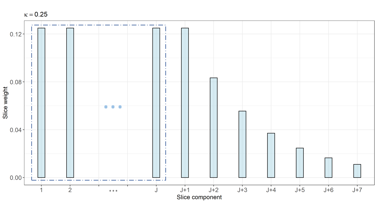
In the definition of a dedicated deterministic sequence , it is crucial to take into account the difference between the manifest and the novel components. Usually, a very common choice is , with . This option allows to compute each analytically, being the smallest integer such that
However, the default choice of a geometrically decreasing -sequence is inappropriate in this context, since we are dealing with a mixture where not all the components are conceptually equivalent. The default -sequence tends to favor components that come first in the mixture specification (in our case, the known ones). To overcome this issue, we propose the following intuitive modification. Given a value for , we equally divide the of the mass into the first elements of the sequence. We then induce a geometric decay in the remaining ones to split the residual fraction . We force the element in position to have the same mass given to the manifest components, to avoid an under-representation of the novelty part. To do so, we define
| (17) |
It is easy to prove that . According to (17), the first elements of the sequence have masses equal to . The truncation threshold changes accordingly, becoming the largest integer such that
| (18) |
Inequality (18) states that the truncation threshold can be only greater or equal to , ensuring that the MCMC always takes into consideration the creation of at least one cluster in the novel distribution. A representation of the modified -sequence is depicted in Figure 2. We report the pseudo-code for the devised Gibbs sampler in the Appendix. The algorithm for the functional extension is not included for conciseness. However, its structure closely follows the one outlined for the multivariate case.
Once the MCMC sample is collected, we first compute the a posteriori probability of being a novelty for every test unit , , that is estimated according to the ergodic mean:
| (19) |
where is the value assumed by the parameter at the -th iteration of the MCMC chain and is the total number of iterations. We remark that the inference on can be conducted directly, since the mixture between the observed components and is not subjected to label switching. In contrast, we need to take this problem into account when dealing with . To perform valid inference, one possibility is to rely on the posterior probability coclustering matrix (PPCM) as indicated in Section 2.3. Each entry of this matrix is estimated as
| (20) |
Once we obtain the PPCM, we employ it to estimate the best partition (BP) in the novelty subset. Indeed, one can recover the BP by minimizing a loss function defined over the space of partitions, which can be computed starting from the PPCM. A famous loss function was proposed by Binder 1978, and investigated in a BNP setting by Lau & Green 2007. However, the so-called Binder loss presents peculiar asymmetries, preferring to split clusters over merging. These asymmetries could result in a number of estimated clusters higher than needed. Therefore, we adopt the Variation of Information (VI - Meilǎ 2007) as loss criterion. The associated loss function, recently proposed by Wade & Ghahramani 2018, is known to provide less fragmented results.
Finally, once the BP for the novelty component has been estimated, we can rely on a heuristic based on the cluster sizes to discriminate anomalies from actual new classes. Let us suppose that the BP consists of novel clusters. Denote the number of instances assigned to cluster with . A cluster is considered to be an agglomerate of outlying points if its cardinality is sufficiently small in comparison to the entire novelty sample size, otherwise it is regarded as a proper novel group.
6 Applications
6.1 Simulation Study
In this section, we present a simulation study aimed at highlighting the capabilities of the new semiparametric Bayesian model in performing novelty detection and we compare it with existing methodologies. We consider different scenarios varying the sample sizes of the hidden classes and the adulteration proportions in the training set. At the same time, we evaluate the importance of the robust information extraction phase and how it affects the learning procedure.
6.1.1 Experimental setup
We consider a training set formed by observed classes, each distributed according to a bivariate Normal density , , with the following parameters:
The class sample sizes are, respectively, equal to , and . The same groups are also present in the test set, together with four previously unobserved classes. We generate the new classes via bivariate Normal densities with parameters:
The test set encompasses a total of components: 3 observed and 4 novelties. Starting from the above-described data generating process, we consider four different scenarios varying:
- •
Data contamination level
- –
No contamination in the training set (Label noise = False)
- –
label noise between classes and (Label noise = True)
- –
- •
Test set sample size
- –
Novelty subset size equal to slightly more than of the test set (Novelty size = Not small)
- –
Novelty subset size equal to of the test set (Novelty size = Small)
- –
Figure 3 exemplifies the experiment structure displaying a realization from the Label noise = True, Novelty size = Not small scenario. As it is evident from the plots, the label noise is strategically included to cause a more difficult identification of the fourth class, should the parameters of the second and third classes be non-robustly learned. Further, notice that the last group presents limited sample size and variability: it could easily be regarded as pointwise contamination (i.e., an anomaly) rather than an actual new component. Nonetheless, following the reasoning outlined in the introduction, we are interested in evaluating the ability of the nonparametric density to capture and discriminate these types of peculiar patterns as well. For each combination of contamination level and test set sample size, we simulate datasets. Results are reported in the following subsection.
6.1.2 Simulation results
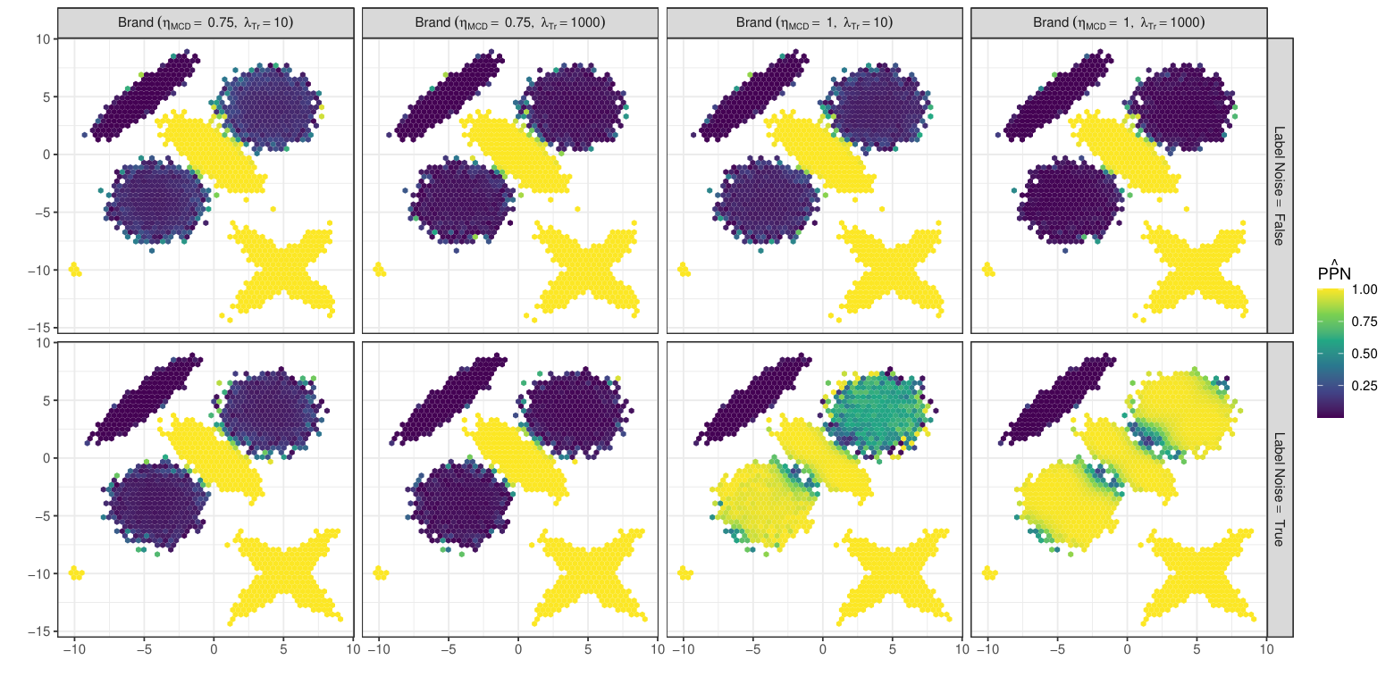
We compare the performance of the Brand model with different hyper-parameters specifications:
- •
the information from the training set is either non-robustly () or robustly () extracted,
- •
the precision parameter associated with the training prior belief is either very high () or moderately low ().
In addition, two model-based adaptive classifiers are considered in the comparison, namely the inductive RAEDDA model (Cappozzo et al. 2020) with labeled and unlabeled trimming levels respectively equal to and , and the inductive AMDA model (Bouveyron 2014). For each replication of the simulated experiment, a set of four metrics is recorded from the test set:
- •
Novelty predictive value (Precision): the proportion of units marked as novelties by a given method truly belonging to classes ,
- •
Accuracy on the observed classes subset: the classification accuracy of a given method within the subset of groups already observed in the training set,
- •
Adjusted Rand Index (ARI, Rand 1971): measuring the similarity between the partition returned by a given method and the underlying true structure,
- •
PPN: a posteriori probability of being a novelty, computed according to Equation (19) (Brand only).
We run MCMC iterations and discard the first as a burn-in phase. Apart from the hyper-parameters for the training components, fairly uninformative priors are employed in the base measure , with and . Lastly, a Gamma DP concentration parameter is considered with prior rate and scale hyper-parameters both equal to .
Figure 4 reports the results for repetitions of the experiment under the different simulated scenarios. A Table containing the values on which this plot is built is deferred to the Supplementary Material. The Novelty predictive value metric highlights the capability of the model to correctly recover and identify the previously unseen patterns. As expected, in the adulteration-free scenarios, all methodologies succeed well enough in separating known and hidden components. The worst performance is exhibited by the RAEDDA model for which, due to the fixed trimming level, a small part of the group-wise most extreme (but still genuine) observations is discarded, thus slightly overestimating the novelties percentage (the same happens for the ARI metric). Different results are displayed in scenarios wherein the label noise complicates the learning process. Robust procedures efficiently cope with the adulteration present in the training set, while the AMDA and the Brand methods when tend to largely overestimate the novelty component. Particularly, the harmful effect caused by the mislabeled units is exacerbated in the Brand model that sets high confidence in the priors , while a partial mitigation, albeit feeble, emerges when is set equal to . This consequence is even more apparent in the hex plots of Figure 5, where we see that the latter model tries to modify its prior belief to accommodate the (outlier-free) test units, while the former, forced to stick close to its prior distribution by the high value of , incorporates the second and third class in the novelty term. The final output, as displayed in the Accuracy on the observed classes subset boxplots, has an overall high misclassification error when it comes to identifying the test units belonging to the previously observed classes. Differently, setting robust informative priors prevents this undesirable behavior, as it is shown by both the high level of accuracy and the associated low posterior probability of being a novelty in the feature space wherein the observed groups lie. On the other hand, the true partition recovery, assessed by the Adjusted Rand Index, does not seem to be influenced by the label noise, with our proposal always outperforming the competing methodologies regardless of which hyper-parameters are selected. As previously mentioned, for and cases the second and third classes are assimilated into the nonparametric component in the Label Noise = True scenario. This is due to the fact that the mislabeled units prevent Brand from correctly learning the true structures of groups two and three in Stage I. As a consequence, no correspondence between these improperly estimated classes in the training is found in the test set, so much so that the DP prior creates them anew within the novelty term. Clearly, this is a sub-optimal behavior as the separation of what is known from what is novel is completely lost, yet it may raise suspicion on dealing with a contaminated learning set, suggesting the need of a robust prior information extraction.
Additional simulated experiments, involving a high-dimensional scenario and novelty detection problem under model misspecification are included in the Supplementary Material.
6.2 X-ray images of wheat kernels
Sophisticated and advanced techniques like X-rays, scanning microscopy and laser technology are increasingly employed for the automatic collection and processing of images. Within the domain of computer vision studies, novelty detection is generally portrayed as a one-class classification problem. There, the aim is to separate the known patterns from the absent, poorly sampled or not well defined remainder (Khan & Madden 2014). Thus, there is strong interest in developing methodologies that not only distinguish the already observed quantities from the new entities, but that also identify specific structures within the novelty component.
The present case study involves the detection of a novel grain type by means of seven geometric parameters, recorded postprocessing X-ray photograms of kernels (Charytanowicz et al. 2010). In more detail, for the samples belonging to the three different wheat varieties, high quality visualization of the internal kernel structure is detected using a soft X-ray technique and, subsequently, the image files are post-processed via a dedicated computer software package (Strumio et al. 1999). The obtained dataset is publicly available in the University of California, Irvine Machine Learning data repository. This experiment involves the random selection of training units from the first two cultivars, and a test set of samples, including grains from the third variety. The resulting learning scenario is displayed in Figure 6. The aim of the analysis is to employ Brand to detect the third unobserved variety, whilst performing classification of the known grain types with high accuracy. Firstly, the MCD estimator with hyper-parameter is adopted for robustly learning the training structure of the two observed wheat varieties. In the second stage, our model is fitted to the test set, discarding iterations for the burn-in phase, and subsequently retaining MCMC samples. As usual, fairly uninformative priors are employed in the base measure , with and , where denotes the 7-dimensional zero vector. For the training components, mean and covariance matrices of the Normal-inverse-Wishart priors are directly determined by the MCD output of the first stage, while and are specified to be respectively equal to and . The latter value indicates that after having robustly extracted information for the two observed classes, high trust is placed in the prior distributions of the known components. Model results are reported in Figure 7, where the posterior probability of being a novelty , , displayed in the plots below the main diagonal, are estimated according to the ergodic mean in (19). The a posteriori classification, computed via majority vote, is depicted in the plots above the main diagonal, where the water-green solid diamonds denote observations belonging to the novel class. The confusion matrix associated with the estimated group assignments is reported in Table 1, where the third group variety is effectively captured by the flexible process modeling the novel component.
| Truth | |||
|---|---|---|---|
| Classification | 1 | 2 | 3 |
| 1 | 30 | 0 | 7 |
| 2 | 2 | 35 | 0 |
| New | 3 | 0 | 28 |
All in all, the promising results obtained with this multivariate dataset may foster the employment of our methodology in automatic image classification procedures that supersede the one-class classification paradigm, allowing for a much more flexible anomaly and novelty detector in computer vision applications.
6.3 Functional novelty detection of meat variety
In recent years, machine learning methodologies have experienced an ever-growing interest in countless fields, including food authentication research (Singh & Domijan 2019). An authenticity study aims to characterize unknown food samples, correctly identifying their type and/or provenance. Clearly, no observation is to be trusted in a context wherein the final purpose is to detect potentially adulterated units, in which, for example, an entire subsample may belong to a previously unseen pattern. Motivated by a dataset of Near Infrared Spectra (NIR) of meat varieties, we employ the functional model introduced in Section 4 to perform classification and novelty detection when having a hidden class and four manually adulterated units in the test set. The considered data report the electromagnetic spectrum for a total of homogenized meat samples, recorded from at intervals of (McElhinney et al. 1999). The units belong to five different meat types, with beef, chicken, lamb, pork, and turkey records. The amount of light absorbed at a given wavelength is recorded for each meat sample: where is the reflectance value. The visible part of the electromagnetic spectrum ( ) accounts for color differences in the meat types, while their chemical composition is recorded further along the spectrum. NIR data can be interpreted as a discrete evaluation of a continuous function in a bounded domain. Therefore, the procedure described in Section 4 is a sensible methodological tool for modeling this type of data objects (Barati et al. 2013). We randomly partition the recorded units into labeled and unlabeled sets. The former includes chicken, lamb, pork, and turkey samples. The latter contains the same proportion of these four meat types with an additional beef units. The last class is not observed in the test set and needs to be discovered. Also, four validation units are manually adulterated and added to the test set as follows:
- •
a shifted version of a pork sample, achieved by removing the first data points and appending the last group-mean absorbance values at the end of the spectrum;
- •
a noisy version of a pork sample, generated by adding Gaussian white noise to the original spectrum;
- •
a modified version of a turkey sample, obtained by abnormally increasing the absorbance value in a single specific wavelength to simulate a spike;
- •
a pork sample with an added slope, produced by multiplying the original spectrum by a positive constant.
These modifications mimic the ones considered in the “Chimiométrie 2005” chemometric contest, where participants were tasked to perform discrimination and outlier detection of mid-infrared spectra of four different starches types (Fern“’andez Pierna & Dardenne 2007). In our context, both the beef subpopulation and the adulterated units are previously unseen patterns that shall be captured by the novelty component.

Firstly, we extract robust prior information from the learning set. Given the spectra non-cyclical nature, we approximate each training unit via a linear combination of B-spline bases, and their associated coefficients are retrieved. Given the high-dimensional nature of the smoothing process, the MRCD is employed to obtain robust group-wise estimates for the splines coefficients. These quantities, which are linearly combined with the B-spline bases, account for the training atoms , specified in Equation (11). We adopt a value of in the first stage, providing functional atoms robust against contamination that may arise in the training set. In this experiment, an inductive approach is considered, for which the training estimates will be kept fixed throughout the subsequent Bayesian learning phase. We further set and , inducing low variability on the noise parameters as much as not to compromise the hierarchical structure between known and novelty components. A more detailed discussion on the hyperparameters choice is deferred to the Supplementary Material, where we evaluate alternative effects for different prior settings within a controlled experiment. Once , are retained, the Bayesian model of Section 4 is applied to the test units running a total of 20,000 iterations and discarding the first 10,000 as warm-up. Figure 8 summarizes the results of the fitted model. Each spectrum is colored according to its a posteriori probability of being a novelty, computed as in (19). The resulting confusion matrix is reported in Table 2, where it is apparent that the previously unseen class, as well as the adulterated units (labeled as “Outliers” in the table), are successfully captured by the novelty component. The obtained classification accuracy is in agreement with the ones produced by state-of-the-art classifiers in a fully-supervised scenario (see, for example, Murphy et al. 2010; Guti“’errez et al. 2014). That is, our proposal is capable of detecting previously unseen classes and outlying units, whilst maintaining competitive predictive power.
| Truth | ||||||
|---|---|---|---|---|---|---|
| Classification | Beef | Chicken | Lamb | Pork | Turkey | Outliers |
| Novelty | 32 | 0 | 0 | 0 | 2 | 4 |
| Chicken | 0 | 21 | 0 | 1 | 12 | 0 |
| Lamb | 0 | 0 | 17 | 0 | 0 | 0 |
| Pork | 0 | 4 | 0 | 20 | 3 | 0 |
| Turkey | 0 | 2 | 0 | 3 | 9 | 0 |
Looking at the classification performance, we observe that Brand can correctly recover the underlying data partition, except for the turkey subgroup. Specifically, the model struggles to separate the turkey units from the chicken ones. Figure 9 provides an explanation for this issue. The left panel shows the robust functional means extracted from the training set. The right panel shows the functional test objects containing the two types of poultry. The overlapping is evident in both cases and it is the main reason why Brand merges the two different sets.
Focusing on the novelty component, the model entirely captures the beef hidden class and the adulterated units, yet two turkey samples are also incorrectly assigned. The obtained classification for the curves identified to be novelties, resulting by VI minimization, is displayed in the left panel of Figure 10, where two distinct clusters are detected. Interestingly, Brand separates the beef samples (blue dashed lines) from the two turkeys (solid red lines) and classifies three of the four manually adulterated units to the outlying cluster. In contrast, the remaining one is assigned to the beef class, because of its peculiar shape, as it is shown in Figure 13 of the Supplementary Material.
Finally, we investigate why two turkey units are incorrectly assigned to the novel component. A closer look at the turkey sub-population, displayed in the right panel of Figure 10, shows how these two samples exhibit a somehow extreme pattern within their group and can, therefore, be legitimately flagged as outlying or anomalous turkeys.
We report two additional figures in the Supplementary Material. The first provides a visual summary of the estimated grouping; the second shows how the turkey test units are partitioned into different clusters.
In this section, we have shown the effectiveness of our methodology in correctly identifying a hidden group in a functional setting, while jointly achieving good classification accuracy and detection of outlying curves. The successful application of the model seems particularly desirable in fields like food authenticity, where generally there is no a priori available information on how many modifications and/or adulteration mechanisms may be present in the samples.
7 Conclusion and discussion
We have introduced a two-stage methodology for robust Bayesian semiparametric novelty detection.
In the first stage, we robustly extract the observed group structure from the training set. In the second stage, we incorporate such prior knowledge in a contaminated mixture, wherein we have employed a nonparametric component to describe the novelty term. The latter could either correspond to anomalies or actual new groups. This distinction is made possible by retrieving the best partition within the novel subset. We have investigated the properties of the random measure underlying the model and its connections with existing methods. Subsequently, the general multivariate methodology has been extended to handle functional data objects, resulting in a novelty detector for functional data analysis. A dedicated slice-efficient sampler, taking into account the difference between unseen and seen components, has been devised for posterior inference. An extensive simulation study and applications on multivariate and functional data have validated the effectiveness of our proposal, fostering its employment in diverse areas from image analysis to chemometrics.
Brand can represent the starting point for many different research avenues. Future research directions aim at providing a Bayesian interpretation of the robust MCD estimator to propose a unified, fully Bayesian model. More versatile specifications can be adopted for the known components, weakening the Gaussianity assumption. These extensions can be obtained by adopting more flexible distributions while keeping the mean and variance of the resulting densities constrained to the findings in the training set, for example, via centered stick-breaking mixtures (Yang et al. 2010).
Similarly, functional Brand can be improved by adopting a more general prior specification via Gaussian Processes (Rasmussen & Williams 2005). Lastly, it is of paramount interest to develop scalable algorithms, as Variational Bayes (Blei et al. 2017) and Expectation-Maximization (Dempster et al. 1977), for inference on massive datasets. Such solutions will offer both increased speed and lower computational cost, which are crucial for assuring the applicability of our proposal in the big data era.
8 Supporting Information
The Supplementary Material referenced throughout the article is available with this paper at the Statistics and Computing website. As supporting information, we report the proofs of the theoretical results showed in Section 3. Moreover, to complement the results presented in Section 6, we showcase the performance obtained by applying Brand to various challenging simulated data, varying the distributional assumptions and dimensionality. We also discuss an application to a higher dimensional real dataset, the popular benchmark Wine dataset from the UCI dataset repository, considering all its 13 features. Lastly, with the help of a controlled experiment, we guide the reader through the choice of hyperparameters and, more broadly, the whole usage of the model in the functional case. Software routines, including the implementation for both methods, the simulation study, and real data analyses of Section 6 are openly available at github.com/AndreaCappozzo/brand-public_repo.
Acknowledgement
The authors want to thank the Editor and the anonymous Reviewers for their suggestions and comments, which significantly improved the scientific value of the manuscript. During the development of this article, F. Denti was funded as a postdoctoral scholar by the NIH grant R01MH115697. Previously, he was also supported as a Ph.D. student by University of Milano - Bicocca, Milan, Italy and Università della Svizzera italiana, Lugano, Switzerland. Andrea Cappozzo and Francesca Greselin’s work was supported by Milano-Bicocca University Fund for Scientific Research, 2019-ATE-0076
Appendix
2. Compute the stochastic truncation term according to (18).
3. Let with . Sample from a conjugate Dirichlet distribution:
5. Compute the SB weights according to (5)
6. Compute the one-line probability weights according to (14).
7. Sample the atoms for the observed classes exploiting conjugacy between the likelihood and the prior for .
8. Sample the atoms for the novel classes exploiting conjugacy between the likelihood and the prior for .
9. Obtain concatenating the updated values of and .
10. Sample each from the following joint discrete distribution:
11. Recover the values for the membership vectors and using (15). Divide the elements in into and . end for
References
- Abraham et al. (2003) C. Abraham, P.. Cornillon, Eric Matzner-Lber and N. Molinari “Unsupervised curve clustering using B-splines” In Scandinavian Journal of Statistics 30.3, 2003, pp. 581–595 DOI: 10.1111/1467-9469.00350
- Aeberhard et al. (1993) Stefan Aeberhard, Danny Coomans and Olivier Vel “Improvements to the classification performance of RDA” In Journal of Chemometrics 7.2, 1993, pp. 99–115 DOI: 10.1002/cem.1180070204
- Akhanli & Hennig (2020) Serhat Akhanli and Christian Hennig “Comparing clusterings and numbers of clusters by aggregation of calibrated clustering validity indexes” In Statistics and Computing 30.5 Springer US, 2020, pp. 1523–1544 DOI: 10.1007/s11222-020-09958-2
- Barati et al. (2013) Zeinab Barati, Issa Zakeri and Kambiz Pourrezaei “Functional data analysis view of functional near infrared spectroscopy data” In Journal of Biomedical Optics 18.11, 2013, pp. 117007 DOI: 10.1117/1.JBO.18.11.117007
- Bigelow & Dunson (2009) Jamie. Bigelow and David. Dunson “Bayesian semiparametric joint models for functional predictors” In Journal of the American Statistical Association 104.485, 2009, pp. 26–36 DOI: 10.1198/jasa.2009.0001
- Binder (1978) D.. Binder “Bayesian Cluster Analysis” In Biometrika 65.1, 1978, pp. 31 DOI: 10.2307/2335273
- Blei et al. (2017) David. Blei, Alp Kucukelbir and Jon. McAuliffe “Variational Inference: A Review for Statisticians” In Journal of the American Statistical Association 112.518 Taylor & Francis, 2017, pp. 859–877 DOI: 10.1080/01621459.2017.1285773
- Boor (2001) Carl de Boor “A Practical Guide to Splines - Revised Edition” In Springer-Verlag, New York, 2001
- Boudt et al. (2020) Kris Boudt, Peter. Rousseeuw, Steven Vanduffel and Tim Verdonck “The minimum regularized covariance determinant estimator” In Statistics and Computing 30.1, 2020, pp. 113–128 DOI: 10.1007/s11222-019-09869-x
- Bouveyron (2014) Charles Bouveyron “Adaptive mixture discriminant analysis for supervised learning with unobserved classes” In Journal of Classification 31.1, 2014, pp. 49–84 DOI: 10.1007/s00357-014-9147-x
- Butler et al. (1993) R.. Butler, P.. Davies and M. Jhun “Asymptotics for the Minimum Covariance Determinant Estimator” In The Annals of Statistics 21.3, 1993, pp. 1385–1400 DOI: 10.1214/aos/1176349264
- Canale et al. (2017) A Canale, A Lijoi, B Nipoti and I Pr“”unster “On the Pitman-Yor process with spike and slab base measure” In Biometrika 104.3, 2017, pp. 681–697 DOI: 10.1093/biomet/asx041
- Cappozzo et al. (2020) Andrea Cappozzo, Francesca Greselin and Thomas Murphy “Anomaly and Novelty detection for robust semi-supervised learning” In Statistics and Computing 30.5, 2020, pp. 1545–1571 DOI: 10.1007/s11222-020-09959-1
- Carpenter et al. (1997) Gail Carpenter, Mark Rubin and William Streilein “ARTMAP-FD: familiarity discrimination applied to radar target recognition” In Proceedings of International Conference on Neural Networks (ICNN’97) 3, 1997, pp. 1459–1464 IEEE
- Cator & Lopuha“”a (2012) Eric. Cator and Hendrik. Lopuha“”a “Central limit theorem and influence function for the MCD estimators at general multivariate distributions” In Bernoulli 18.2, 2012, pp. 520–551 DOI: 10.3150/11-BEJ353
- Charytanowicz et al. (2010) Magorzata Charytanowicz et al. “Complete gradient clustering algorithm for features analysis of X-ray images” In Advances in Intelligent and Soft Computing 69, 2010, pp. 15–24 DOI: 10.1007/978-3-642-13105-9˙2
- Croux & Haesbroeck (1999) Christophe Croux and Gentiane Haesbroeck “Influence Function and Efficiency of the Minimum Covariance Determinant Scatter Matrix Estimator” In Journal of Multivariate Analysis 71.2, 1999, pp. 161–190 DOI: 10.1006/jmva.1999.1839
- De Blasi et al. (2020) Pierpaolo De Blasi, Asael Mart“’inez, Rams“’es. Mena and Igor Pr“”unster “On the inferential implications of decreasing weight structures in mixture models” In Computational Statistics and Data Analysis 147, 2020 DOI: 10.1016/j.csda.2020.106940
- Dempster et al. (1977) A Dempster, N. Laird and D Rubin “Maximum likelihood from incomplete data via the EM algorithm” In Journal of the Royal Statistical Society 39.1, 1977, pp. 1–38 DOI: http://dx.doi.org/10.2307/2984875
- Escobar & West (1995) Michael. Escobar and Mike West “Bayesian Density Estimation and Inference Using Mixtures” In Journal of the American Statistical Association 90.430, 1995, pp. 577–588 DOI: 10.1080/01621459.1995.10476550
- Ferguson (1973) Thomas. Ferguson “A Bayesian Analysis of Some Nonparametric Problems” In The Annals of Statistics 1.2 The Annals of Statistics, 1973, pp. 209–230 DOI: 10.1214/aos/1176342360
- Fern“’andez Pierna & Dardenne (2007) Juan Fern“’andez Pierna and Pierre Dardenne “Chemometric contest at ‘Chimiométrie 2005’: A discrimination study” In Chemometrics and Intelligent Laboratory Systems 86.2, 2007, pp. 219–223 DOI: 10.1016/j.chemolab.2006.06.009
- Fop et al. (2021) Michael Fop, Pierre-Alexandre Mattei, Charles Bouveyron and Thomas Murphy “Unobserved classes and extra variables in high-dimensional discriminant analysis”, 2021 arXiv: http://arxiv.org/abs/2102.01982
- Forina et al. (1986) M Forina, C Armanino, M Castino and M Ubigli “Multivariate data analysis as a discriminating method of the origin of wines” In Vitis 25.3, 1986, pp. 189–201
- Gordaliza (1991) Alfonso Gordaliza “Best approximations to random variables based on trimming procedures” In Journal of Approximation Theory 64.2, 1991, pp. 162–180 DOI: 10.1016/0021-9045(91)90072-I
- Guti“’errez et al. (2014) Luis Guti“’errez, Eduardo Guti“’errez-Pe“˜na and Rams“’es. Mena “Bayesian nonparametric classification for spectroscopy data” In Computational Statistics and Data Analysis 78, 2014, pp. 56–68 DOI: 10.1016/j.csda.2014.04.010
- Hennig (2015) Christian Hennig “What are the true clusters?” In Pattern Recognition Letters 64, 2015, pp. 53–62 DOI: 10.1016/j.patrec.2015.04.009
- Hubert & Debruyne (2010) Mia Hubert and Michiel Debruyne “Minimum covariance determinant” In Wiley interdisciplinary reviews: Computational statistics 2.1 Wiley Online Library, 2010, pp. 36–43
- Hubert et al. (2018) Mia Hubert, Michiel Debruyne and Peter. Rousseeuw “Minimum covariance determinant and extensions” In Wiley Interdisciplinary Reviews: Computational Statistics 10.3, 2018, pp. 1–11 DOI: 10.1002/wics.1421
- Hubert & Van Driessen (2004) Mia Hubert and Katrien Van Driessen “Fast and robust discriminant analysis” In Computational Statistics & Data Analysis 45.2, 2004, pp. 301–320 DOI: 10.1016/S0167-9473(02)00299-2
- Ishwaran & James (2001) Hemant Ishwaran and Lancelot. James “Gibbs Sampling Methods for Stick-Breaking Priors” In Journal of the American Statistical Association 96.453, 2001, pp. 161–173 DOI: 10.1198/016214501750332758
- Kalli et al. (2011) Maria Kalli, Jim Griffin and Stephen Walker “Slice sampling mixture models” In Statistics and Computing 21.1, 2011, pp. 93–105 DOI: 10.1007/s11222-009-9150-y
- Khan & Madden (2014) Shehroz. Khan and Michael. Madden “One-class classification: taxonomy of study and review of techniques” In The Knowledge Engineering Review 29.3, 2014, pp. 345–374 DOI: 10.1017/S026988891300043X
- Lau & Green (2007) John. Lau and Peter. Green “Bayesian model-based clustering procedures” In Journal of Computational and Graphical Statistics 16.3, 2007, pp. 526–558 DOI: 10.1198/106186007X238855
- Lo (1984) Albert. Lo “On a Class of Bayesian Nonparametric Estimates: I. Density Estimates” In The Annals of Statistics 12.1, 1984, pp. 351–357 URL: https://www.jstor.org/stable/pdf/2241054.pdf
- Malsiner-Walli et al. (2016) Gertraud Malsiner-Walli, Sylvia Fr“”uhwirth-Schnatter and Bettina Gr“”un “Model-based clustering based on sparse finite Gaussian mixtures” In Statistics and Computing 26.1-2 Springer US, 2016, pp. 303–324 DOI: 10.1007/s11222-014-9500-2
- Manikopoulos & Papavassiliou (2002) Constantine Manikopoulos and Symeon Papavassiliou “Network intrusion and fault detection: a statistical anomaly approach” In IEEE Communications Magazine 40.10 IEEE, 2002, pp. 76–82
- Maronna & Yohai (2017) Ricardo Maronna and Victor Yohai “Robust and efficient estimation of multivariate scatter and location” In Computational Statistics and Data Analysis 109, 2017, pp. 64–75 DOI: 10.1016/j.csda.2016.11.006
- McElhinney et al. (1999) John McElhinney, Gerard Downey and Tom Fearn “Chemometric processing of visible and near infrared reflectance spectra for species identification in selected raw homogenised meats” In Journal of Near Infrared Spectroscopy 7.3, 1999, pp. 145–154 DOI: 10.1255/jnirs.245
- Meilǎ (2007) Marina Meilǎ “Comparing clusterings-an information based distance” In Journal of Multivariate Analysis 98.5, 2007, pp. 873–895 DOI: 10.1016/j.jmva.2006.11.013
- Miller & Browning (2003) D.J. Miller and John Browning “A mixture model and EM algorithm for robust classification, outlier rejection, and class discovery” In 2003 IEEE International Conference on Acoustics, Speech, and Signal Processing, 2003. Proceedings. (ICASSP ’03). 2.11 IEEE, 2003, pp. II–809–12 DOI: 10.1109/ICASSP.2003.1202490
- Murphy et al. (2010) Thomas Murphy, Nema Dean and Adrian Raftery “Variable selection and updating in model-based discriminant analysis for high dimensional data with food authenticity applications” In The Annals of Applied Statistics 4.1, 2010, pp. 396–421 DOI: 10.1214/09-AOAS279
- Petrone et al. (2009) Sonia Petrone, Michele Guindani and Alan. Gelfand “Hybrid dirichlet mixture models for functional data” In Journal of the Royal Statistical Society. Series B: Statistical Methodology 71.4, 2009, pp. 755–782 DOI: 10.1111/j.1467-9868.2009.00708.x
- Pitman (1995) Jim Pitman “Exchangeable and partially exchangeable random partitions” In Probability Theory and Related Fields 102.2, 1995, pp. 145–158 DOI: 10.1007/BF01213386
- Pitman & Yor (1997) Jim Pitman and Marc Yor “The two-parameter Poisson-Dirichlet distribution derived from a stable subordinator” In Annals of Probability 25.2, 1997, pp. 855–900 DOI: 10.1214/aop/1024404422
- Ramsay, James, Silverman (2005) B. Ramsay, James, Silverman “Functional Data Analysis” In Springer Series in Statistics, Springer Series in Statistics New York: Springer-Verlag, 2005 DOI: 10.1007/b98888
- Rand (1971) William Rand “Objective criteria for the evaluation of clustering methods” In Journal of the American Statistical Association 66.336, 1971, pp. 846 DOI: 10.2307/2284239
- Rasmussen & Williams (2005) Carl Rasmussen and Christopher K.. Williams “Gaussian Processes for Machine Learning (Adaptive Computation and Machine Learning)” The MIT Press, 2005
- Rigon (2019) Tommaso Rigon “An enriched mixture model for functional clustering” In arXiv, 2019 arXiv: http://arxiv.org/abs/1907.02493
- Ritter (2014) Gunter Ritter “Robust Cluster Analysis and Variable Selection” ChapmanHall/CRC, 2014 DOI: 10.1201/b17353
- Rodriguez & Dunson (2014) Abel Rodriguez and David. Dunson “Functional clustering in nested designs: Modeling variability in reproductive epidemiology studies” In Annals of Applied Statistics 8.3, 2014, pp. 1416–1442 DOI: 10.1214/14-AOAS751
- Rousseau & Mengersen (2011) Judith Rousseau and Kerrie Mengersen “Asymptotic behaviour of the posterior distribution in overfitted mixture models” In Journal of the Royal Statistical Society. Series B: Statistical Methodology 73.5, 2011, pp. 689–710 DOI: 10.1111/j.1467-9868.2011.00781.x
- Rousseeuw (1984) Peter Rousseeuw “Least median of squares regression” In Journal of the American statistical association 79.388 Taylor & Francis, 1984, pp. 871–880
- Rousseeuw & Driessen (1999) Peter. Rousseeuw and Katrien Driessen “A fast algorithm for the minimum covariance determinant estimator” In Technometrics 41.3, 1999, pp. 212–223 DOI: 10.1080/00401706.1999.10485670
- Scarpa & Dunson (2009) Bruno Scarpa and David. Dunson “Bayesian hierarchical functional data analysis via contaminated informative priors” In Biometrics 65.3, 2009, pp. 772–780 DOI: 10.1111/j.1541-0420.2008.01163.x
- Sethuraman (1994) Jayaram Sethuraman “A constructive definition of Dirichlet Process prior” In Statistica Sinica 4.2 Institute of Statistical Science, Academia Sinica, 1994, pp. 639–650 URL: http://www.jstor.org/stable/24305538
- Singh & Domijan (2019) Manokamna Singh and Katarina Domijan “Comparison of Machine Learning Models in Food Authentication Studies” In 2019 30th Irish Signals and Systems Conference (ISSC) IEEE, 2019, pp. 1–6 DOI: 10.1109/ISSC.2019.8904924
- Strumio et al. (1999) A. Strumio et al. “Computer system for analysis of x-ray images of wheat grains (a preliminary announcement)” In International Agrophysics 13.1, 1999, pp. 133–140
- Tarassenko et al. (1995) L. Tarassenko, P. Hayton, N. Cerneaz and M. Brady “Novelty detection for the identification of masses in mammograms” In IEE Conference Publication, 1995, pp. 442–447 DOI: 10.1049/cp:19950597
- Tax & Duin (1998) David Tax and Robert Duin “Outlier detection using classifier instability” In Joint IAPR international workshops on statistical techniques in pattern recognition (SPR) and structural and syntactic pattern recognition (SSPR), 1998, pp. 593–601 Springer
- Todorov & Filzmoser (2009) Valentin Todorov and Peter Filzmoser “An Object-Oriented Framework for Robust Multivariate Analysis” In Journal of Statistical Software 32.3, 2009, pp. 1–47 DOI: 10.18637/jss.v032.i03
- Wade & Ghahramani (2018) Sara Wade and Zoubin Ghahramani “Bayesian Cluster Analysis: Point estimation and credible balls (with Discussion)” In Bayesian Analysis 13.2, 2018, pp. 559–626 DOI: 10.1214/17-BA1073
- Yang et al. (2010) Mingan Yang, David. Dunson and Donna Baird “Semiparametric Bayes hierarchical models with mean and variance constraints” In Computational Statistics and Data Analysis 54.9, 2010, pp. 2172–2186 DOI: 10.1016/j.csda.2010.03.025
Supplementary Material In this Supplementary Material, we report proofs for the theoretical results reported in the main paper and some additional numerical experiments, for both the multivariate Brand and its functional extension.
9 Proofs
First, we derive the moments, the variance, and the covariance for the simpler case (A): . Then, we derive the same quantities starting from the discrete random measure that underlies Brand (B): .
9.1 Case A:
9.2 Case B:
Let us represent all the possible values of in one vector
| (21) | ||||
10 Multivariate Brand - Additional experiments
The present section integrates and extends the simulation study reported in Section 6.1 of the manuscript. Particularly, the multivariate Brand is applied to a real -dimensional dataset (Section 10.1), and to two additional simulation studies: the former dealing with non-Gaussian shaped components (Section 10.2) and the latter encompassing higher-dimensional, sparse covariance structures (Section 10.3).
10.1 Wine dataset
The dataset, publicly available in the University of California Irvine Machine Learning repository, comprises chemical measurements from wine samples from the Piedmont region, Italy (Forina et al. 1986). The samples arise from three different cultivars: Barolo, Grignolino, and Barbera. We randomly select samples from the first two varieties to build the training set, whereas the remaining samples, including wines from the third cultivar, defines the test set. The multivariate Brand methodology is fitted to the datasets to detect the third unobserved wine type. The model hyper-parameters are set as follows. First, induces robust priors elicitation for the two observed classes. Fairly uninformative priors are used for the base measure , namely and , where with we denote the -dimensional zero vector. Such priors agree with the ones employed in Section 6.2.1 in the main paper for the seed dataset, underlying their general applicability in scenarios where no initial information is available. After initiating the MCMC with iterations for the burn-in phase, dependent samples are retained from the target posterior distribution. The resulting classification is reported in Table 3: our semi-parametric model almost perfectly recovers the underlying partition, efficiently identifying the novel wine type. The derived accuracy is particularly high, with performance comparable to those obtained in fully-supervised experiments (Aeberhard et al. 1993).
| Truth | |||
|---|---|---|---|
| Classification | Barolo | Grignolino | Barbera |
| Barolo | 29 | 0 | 0 |
| Grignolino | 1 | 32 | 2 |
| New | 0 | 0 | 48 |
10.2 Non-Gaussian shaped classes
In this section, we employ the same hyperparameters configuration considered for the experimental setup in Section 6.1.1 of the main paper to generate samples from elliptical distributions that differ from the Gaussian, with the final aim of validating Brand performance under model misspecification. As discussed, the general structure reported in Equation (1) allows for any distributional kernel specification. However, departures from Gaussianity would induce the loss of the conjugacy properties, worsening the computational cost. Therefore, we now want to test how robust the Gaussian kernel is in capturing symmetric components with heavier tails. To this extent, we repeat the experiment for the Label noise = False and Novelty size = Not small scenario, with resulting sample sizes being equal to
and
for the training and test sets, respectively. In contrast to the simulations reported in the main paper, we generate groups to via a multivariate distribution with degrees of freedom, while classes and are realizations from a multivariate Laplace distribution. The resulting learning framework is displayed in Figure 11.
The simulation results, for the same hyper-parameters specification employed in the main paper, are reported in Figure 12. We immediately notice that different prior settings do not substantially influence the overall model performance, with satisfactorily good results showcased for all the considered metrics. Notwithstanding, when we compare the simulation outcome in Figure 12 with the one displayed in Figure 4 of the main paper, it is apparent that the results are in some measure influenced by model misspecification.
In detail, the novelty term tends to absorb all those units sampled from the (heavy) tails of the known components, as they present very low Gaussian density, particularly when . Consequently, the clustering induced by the DPMM shows many more groups a posteriori in this scenario, with singletons trying to accommodate patterns that the main classes cannot explain.
While clearly accuracy measures for assessing the goodness of a clustering procedure shall be application-dependent (Hennig 2015), we argue here that, in principle, the outcome showcased by our method could still be relevant in contexts that violate the Gaussianity assumption. More specifically, if the sought classes are assumed to be unimodal and elliptical, both stages in the brand methodology concur to achieve this result. Stage I trims the group-wise most outlying values, and Stage II flexibly captures all the unexplained variability with Gaussian-like shapes.
Once this has been accomplished, one can employ the output evaluation in terms of trimmed units and a posteriori assignment to determine which assumptions were not met by the dataset at hand. As an example, the identification of small novel clusters in the vicinity of bigger ones may be an indication that components with heavier tails are needed to properly account for the true underlying partition. For a general overview on the difficult problem of finding groups in data and associated clustering validity measures, the interested reader is refered to Akhanli & Hennig 2020.
10.3 High-dimensional heteroscedastic classes
For this experiment, we consider the same number of classes (known and hidden ones) and sample sizes for training and test sets introduced in the previous section. Each component is distributed according to a multivariate Normal density with mean vectors equal to:
and covariance matrices exhibiting different degrees of sparsity, as illustrated in Figure 13.

We display the resulting learning framework in Figure 14, where the training and test samples are reported in the lower and in the upper diagonal plots, respectively. Notice that the generative mechanism induces a quite challenging novelty detection problem, as the last four dimensions are irrelevant for group separation.

By again monitoring the metrics defined in the main manuscript, we aim at investigating the Brand performance when dealing with a -dimensional dataset with heterogeneous covariance patterns. Given the well-established efficacy of both the MCD and RMCD estimators in high-dimensional settings (Rousseeuw & Driessen 1999; Hubert et al. 2018; Boudt et al. 2020), we focus here on the second stage of the Brand method, studying its sensitivity under different hyper-parameters specifications. In detail, a total of models are fitted to simulated datasets varying:
- •
the concentration parameter of the Dirichlet Process prior, letting it be equal to or ,
- •
the degrees of freedom associated with the novelty components, letting it be equal to or ,
- •
the precision parameter associated with the novelty components, letting it be equal to or .
Simulation results are reported in Figure 15. We immediately notice that the overall performance showcased by our methodology is satisfactorily good, regardless of the hyperparameters specification. Both known and novel patterns are correctly identified as such, with results mirroring the ones obtained in the bi-dimensional experiments reported in Section 6.1.2 of the main paper. In particular, eliciting very flat priors for the base measure (, ) still produces excellent outcomes. The only appreciable difference is in terms of ARI, induced by the DP concentration parameter . Specifically, increasing favors a priori the creation of more clusters. As a result, the model is more prone to accommodate components with a limited sample size, like the seventh group in the present experiment. On the other hand, when the test units arisen by the last density are usually merged within some other components, producing the slight difference in ARI visible in the middle plot of Figure 15.
11 Functional Brand - Controlled experiment
This section investigates how functional Brand behaves according to various prior specifications and different levels of noise in the data. We aim to provide the researchers and practitioners with guidelines for the hyperparameter specification to exploit the flexibility of our model at its fullest. In the next experiments, we will consider the following six functions, evaluated on the interval :
Figure 16 provides a visual representation of the six functions. Each of these functions presents its distinctive peculiarities. Simultaneously, they overlap, especially in the left half of the support, which could make the classification more difficult conditioning on the considered noise level. These six functions constitute the functional means of different groups we are going to study.

We suppose that every function is observed on a discretized collection of 100 time points between and . In all our simulation settings, we fix the number of functions sampled from each group to . We assume that samples from the first three groups are contained in both the training set and in the test set , while samples from the last three groups represent the novelties we want to detect, and therefore they appear only in . We are left with data objects in the training sets and in the test sets. More formally, for each group in the training set ntained in both the training set , we have
For each group in the test set , we have
Finally, we assume three different levels of noise in the data generating process, considering , yielding three simulated cases of training and test sets (), () and ().
Figure 17 shows the three generated test sets, stratified by the increasing noise level.
As already mentioned, a higher level of noise induces a more evident overlap among the functional objects. We expect this overlap to make the classification more challenging.

11.1 The robust estimation of the mean function
We focus on Stage I, and we investigate the robust extraction of prior information in the functional case. In the main paper, we discuss how we smooth the training functions using B-splines bases. Similarly, for this study, we use 100 bases of order 5, which provide accurate results for a reasonable computational cost.
Our functional robust estimation works as follows. We first collect the spline coefficients, and we interpret them as multivariate objects. We then apply the MCD estimator on the spline coefficients. We therefore recover, for each group, the robust mean coefficients that, once convoluted with the bases, will produce our mean functions.
A crucial quantity is the percentage of extreme coefficients to remove in our robust estimation. This percentage significantly affects also the recovery of the training noise . In the following, we demonstrate how the ratio of trimmed values affects Stage I in the functional case.
To showcase the effect of the MCD estimator, we contaminate the known classes in the training sets with time-point specific outliers and label noise. In detail, we add noise sampled from to fifteen randomly selected functions at fifteen random timestamps.
We contaminate five functions from the first group, four in the second, and six in the third. Then, we shuffle of the functions across groups to generate label noise. To illustrate this step, we report in Figure 18 a visual depiction of the contaminated version of the training dataset , stratified by class.

We consider three different specifications of :
- •
no trimming by setting : all the estimated spline coefficients are considered;
- •
mild trimming, : only 5% of the estimated spline coefficients are removed for the estimation of the group centroids and functional noise;
- •
strong trimming. : a fourth of the estimated spline coefficients is removed before computing the group centroids and functional noise.
We report the extracted mean functions and the estimated noise in the panels of Figure 19. Specifically, the group centroids are depicted in red, superimposed onto the observations of every group. We also plot in blue the intervals of variation computed as to give an idea of the estimated noise, for . Each column of the plot shows the evolution of the mean and noise functions when considering different trimming levels, stratified by group. We can observe how employing trimming benefits the estimation of the representative functions in each group.
For example, in the first row of Figure 19, we see how the red line fails to represent the group characteristics. This behavior is exacerbated close to the boundaries in all the groups. It is evident how even a small percentage of trimming yields considerable benefits. In our experience, we obtain very satisfactory results in the functional case when considering a strong trimming. Results in a case of extreme trimming, obtained by setting were explored but not reported, since similar to the case . In conclusion, if enough data are available, we suggest considering strong trimming as the safest option when dealing with the functional case. In this way, we can eradicate the influence of potential outliers on both the mean and the variance. We will use the mean and noise functions recovered with for the subsequent analyses.
11.2 Model performance according to different prior specifications
We can summarise the hyperparameters specific of functional Brand in three main subsets:
- •
Subset 1: hyperparameters controlling the dispersion around the extracted mean functions of the known groups: and ;
- •
Subset 2: hyperparameters controlling the dispersion around the novel spline coefficients, representing the unknown mean functions: , , and ;
- •
Subset 3: hyperparameters controlling the dispersion of the noise around the novel mean functions: and .
We investigate the sensitivity of functional Brand to various hyperparameter specifications while considering the different noise levels in the observed data, as previously discussed. As a first consideration, we point out that setting the hyperparameters controlling the variance around the known classes and/or the novel ones requires the most care. A poorly elicited prior for the error terms could lead to losing Brand hierarchical structure, letting the novelty components take over the known groups in lieu of their flexibility. The opposite issue may also arise, since larger mixture weights are assigned to the known components. In the following, we will provide some considerations regarding the tuning of the hyperparameters listed in Subset 1 and Subset 2. For the sake of brevity, we omit the results obtained tweaking the parameters that belong to Subset 3, which control the noise level in the novelty term . Given the insights collected in several applications, we suggest eliciting an Inverse Gamma prior that favors low noise values, promoting more sensitive estimation of the random functions . Thus, we fix and in the following, as well as in the functional application in the main paper.
Let us first discuss the hyperparameter specification that we adopted in the main text. We are going to assume these values as our default setting. The values are
First, let us describe and justify our choice of hyperparamters.
The parameters in Subset 1 are set to negligible values. In this way, we are implicitly enforcing an inductive learning approach: the information extracted from the training set for the known groups is trustworthy and need not be updated.
We calibrate the parameters in Subset 2 to induce a reasonably tight prior over the novel splines coefficients to help the model identifiability. One can claim that an uninformative specification would also be reasonable to reflect our ignorance about the novel groups. However, as we will show, letting the parameters to vary too freely may negatively affect the results.
Finally, as already discussed, the informative specification of the parameters in Subset 3 bounds the variance of the errors around the novel functions: this will avoid limiting cases where all the information contained in the data is explained by the noise term, helping the identification of the latent mean functions.
In the following, we tweak one subset of parameters at a time to investigate its effect, starting from this prior configuration. In all the subsequent experiments, we run 7,500 MCMC iterations after a burn-in period of the same length.
11.2.1 Tuning hyperparameters: Subset 1
For this first experiment, we consider the three hyperprior configurations devised to increase the uncertainty around the functional means and variance extracted from the training set.
In other words, we want to understand how, ceteris paribus, the concentration of the priors for and , affects the estimation of the mean functions of the known groups.
As already mentioned, a proper elicitation of the prior noises for the known classes is crucial for carrying out sensible inference.
Throughout many simulation studies, we observed that plays a fundamental role in preserving the specific hierarchy that characterizes Brand.
In fact, in scenarios where the prior variance of the measurement errors around the training mean is too wide, the known components lose their “priority” over the novel ones. In other words, the robust estimates extracted from the training set are deemed as less representative of the truth. Simultaneously, the flexibility of the novelty terms leaves the new estimated functions free to adapt to the dataset, ending up absorbing the known classes. In short, if the variances of the known components are not carefully tuned, Brand loses the ability to distinguish between known groups and novelties, hindering the resulting classification.
To provide an idea on how different choices of , and affect the results, we consider:
- HPC 1 -
Inductive setting: ,
- HPC 2 -
Informative specification: ,
- HPC 3 -
“Uninformative” specification: . The variance around the mean function is set to 1.
For each configuration, we estimate functional Brand on the three different test sets , , and . We show the confusion matrices displaying the assignation of the functional objects contained in the test set into known classes or novelties in Table 4.
Moreover, to better exemplify the model’s behavior, we display the functional estimates of the known mean functions for in Figure 20. For each known group, we collect the robustly extracted mean functions (in red), the simulated posterior mean
functions (computed pointwise, in blue) on top of the MCMC iterations (in black).
We can detect a recurring pattern across different datasets.
On the one hand, the first and second prior configurations (HPC 1 and HPC 2) lead to perfect classification of the functional data into known components (Classes 1, 2, and 3 into Cluster 1, 2, and 3, respectively) and novelties (Classes 4, 5, and 6 into Cluster 0) regardless the level of noise in the dataset.
Looking at the different panels of Figure 20, we see how HPC 2 allows more uncertainty in the mean estimates (represented by a wider range of variation of the MCMC simulations) and a difference between the starting robust means (in red) and the MCMC posterior means (in blue). As expected, in the inductive setting, the red and blue lines coincide.
On the other hand, we can see what happens when tight constraints are not placed on the variances by focusing on the last block of columns in Table 4 and the last row of panels in Figure 20.
In all the three cases , , and we see how the novelty component takes over and ruins the classification process. For example, in the bottom row of Figure 20 we see that in the three panels the estimated posterior mean function coincides with the prior since no data have been assigned to those components. In the first two datasets, we see how the higher variances lead Brand to mislead a novel group as a known one and viceversa.
We can conclude that, for the functional setting, care is needed when tuning the discussed hyperprior parameters. Thus, when enough data are available, we suggest either to rely on the inductive learning process or, otherwise, to induce small a priori variations.
| HPC 1 | HPC 2 | HPC 3 | |||||||||||||||||
|---|---|---|---|---|---|---|---|---|---|---|---|---|---|---|---|---|---|---|---|
| Ground Truth | 1 | 2 | 3 | 4 | 5 | 6 | 1 | 2 | 3 | 4 | 5 | 6 | 1 | 2 | 3 | 4 | 5 | 6 | |
| 0 | 0 | 0 | 0 | 50 | 50 | 50 | 0 | 0 | 0 | 50 | 50 | 50 | 50 | 50 | 50 | 0 | 50 | 50 | |
| 1 | 50 | 0 | 0 | 0 | 0 | 0 | 50 | 0 | 0 | 0 | 0 | 0 | 0 | 0 | 0 | 50 | 0 | 0 | |
| 2 | 0 | 50 | 0 | 0 | 0 | 0 | 0 | 50 | 0 | 0 | 0 | 0 | 0 | 0 | 0 | 0 | 0 | 0 | |
| 3 | 0 | 0 | 50 | 0 | 0 | 0 | 0 | 0 | 50 | 0 | 0 | 0 | 0 | 0 | 0 | 0 | 0 | 0 | |
| 0 | 0 | 0 | 0 | 50 | 50 | 50 | 0 | 0 | 0 | 50 | 50 | 50 | 50 | 50 | 50 | 0 | 50 | 50 | |
| 1 | 50 | 0 | 0 | 0 | 0 | 0 | 50 | 0 | 0 | 0 | 0 | 0 | 0 | 0 | 0 | 50 | 0 | 0 | |
| 2 | 0 | 50 | 0 | 0 | 0 | 0 | 0 | 50 | 0 | 0 | 0 | 0 | 0 | 0 | 0 | 0 | 0 | 0 | |
| 3 | 0 | 0 | 50 | 0 | 0 | 0 | 0 | 0 | 50 | 0 | 0 | 0 | 0 | 0 | 0 | 0 | 0 | 0 | |
| 0 | 0 | 0 | 0 | 50 | 50 | 50 | 0 | 0 | 0 | 50 | 50 | 50 | 50 | 50 | 50 | 50 | 50 | 50 | |
| 1 | 50 | 0 | 0 | 0 | 0 | 0 | 50 | 0 | 0 | 0 | 0 | 0 | 0 | 0 | 0 | 0 | 0 | 0 | |
| 2 | 0 | 50 | 0 | 0 | 0 | 0 | 0 | 50 | 0 | 0 | 0 | 0 | 0 | 0 | 0 | 0 | 0 | 0 | |
| 3 | 0 | 0 | 50 | 0 | 0 | 0 | 0 | 0 | 50 | 0 | 0 | 0 | 0 | 0 | 0 | 0 | 0 | 0 | |

11.2.2 Tuning hyperparameters: Subset 2
The discussion for this second set of hyperparameters is structured similarly to the one reported in the previous Subsection. We now investigate Brand’s ability to identify and correctly cluster the novelty terms, while tweaking the variability of the prior distributions of and (and, therefore, of ). We consider the following three hyperparameters configurations:
- HPC 1 -
Adopted specification: , ,
- HPC 2 -
Low variability: , ,
- HPC 3 -
High variability: , , .
We have also investigated a more extreme case, , , , for which we omit the results since this extremely uninformative specification resulted in numerical instabilities and poor classification performance.
The first and second hyperprior specifications lead to perfect clustering for all three datasets. We instead report in Table 5 the results obtained on . A tighter prior for the novelty components leads to the misclassification of only few observations (2/300) and the correct detection of the overall cluster structure. Conversely, a wide prior can overrule the hierarchical structure of the model, absorbing known classes into the novelty term.
| HPC 1 | HPC 2 | HPC 3 | |||||||||||||||||
|---|---|---|---|---|---|---|---|---|---|---|---|---|---|---|---|---|---|---|---|
| Ground Truth | 1 | 2 | 3 | 4 | 5 | 6 | 1 | 2 | 3 | 4 | 5 | 6 | 1 | 2 | 3 | 4 | 5 | 6 | |
| CKC | 1 | 50 | 0 | 0 | 0 | 0 | 0 | 50 | 0 | 0 | 0 | 0 | 0 | 50 | 0 | 0 | 0 | 0 | 0 |
| 2 | 0 | 50 | 0 | 0 | 0 | 0 | 0 | 50 | 0 | 0 | 0 | 0 | 0 | 1 | 0 | 0 | 0 | 0 | |
| 3 | 0 | 0 | 50 | 0 | 0 | 0 | 0 | 0 | 49 | 0 | 0 | 0 | 0 | 47 | 0 | 0 | 0 | 0 | |
| CNC | 4 | 0 | 0 | 0 | 50 | 0 | 0 | 0 | 0 | 1 | 50 | 0 | 0 | 0 | 1 | 0 | 50 | 0 | 0 |
| 5 | 0 | 0 | 0 | 0 | 50 | 0 | 0 | 0 | 0 | 0 | 50 | 0 | 0 | 0 | 50 | 0 | 47 | 0 | |
| 6 | 0 | 0 | 0 | 0 | 0 | 50 | 0 | 0 | 0 | 0 | 0 | 49 | 0 | 0 | 0 | 0 | 0 | 50 | |
| ENC | 7 | 0 | 0 | 0 | 0 | 0 | 0 | 0 | 0 | 0 | 0 | 0 | 1 | 0 | 0 | 0 | 0 | 1 | 0 |
| 8 | 0 | 0 | 0 | 0 | 0 | 0 | 0 | 0 | 0 | 0 | 0 | 0 | 0 | 0 | 0 | 0 | 1 | 0 | |
| 9 | 0 | 0 | 0 | 0 | 0 | 0 | 0 | 0 | 0 | 0 | 0 | 0 | 0 | 1 | 0 | 0 | 1 | 0 | |
Overall, we can conclude that Brand is more robust to different hyperprior settings regarding the specification of the novelty components. Our specification (HPC 1) provides a nice balance between the flexibility required by the novelty term and the stability of the results.
12 Additional Figures
12.1 Meat variety dataset analysis

13 Additional Table for the Simulation Study of Section 6.1
| Label noise = False | Label noise = True | |||||
|---|---|---|---|---|---|---|
| Accuracy | ARI | Precision | Accuracy | ARI | Precision | |
| Novelty Size = Not small | ||||||
| 0.999 | 0.932 | 0.998 | 0.562 | 0.814 | 0.519 | |
| (0.002) | (0.014) | (0.004) | (0.223) | (0.03) | (0.215) | |
| 0.966 | 0.885 | 0.934 | 0.996 | 0.924 | 0.992 | |
| (0.029) | (0.041) | (0.051) | (0.003) | (0.003) | (0.005) | |
| 0.998 | 0.93 | 0.997 | 0.309 | 0.931 | 0.4 | |
| (0.001) | (0.005) | (0.002) | (0.001) | (0.002) | (0.001) | |
| 0.995 | 0.927 | 0.992 | 0.465 | 0.931 | 0.481 | |
| (0.001) | (0.005) | (0.002) | (0.206) | (0.01) | (0.13) | |
| 0.99 | 0.928 | 0.985 | 0.997 | 0.93 | 0.995 | |
| (0.007) | (0.007) | (0.013) | (0.004) | (0.008) | (0.009) | |
| 0.997 | 0.928 | 0.994 | 0.994 | 0.927 | 0.99 | |
| (0.001) | (0.005) | (0.002) | (0.001) | (0.007) | (0.001) | |
| Novelty Size = Small | ||||||
| 0.999 | 0.986 | 0.996 | 0.69 | 0.905 | 0.459 | |
| (0.002) | (0.004) | (0.011) | (0.29) | (0.026) | (0.353) | |
| 0.969 | 0.947 | 0.855 | 0.996 | 0.981 | 0.977 | |
| (0.015) | (0.019) | (0.06) | (0.003) | (0.003) | (0.014) | |
| 0.998 | 0.986 | 0.994 | 0.413 | 0.986 | 0.23 | |
| ( 0.01) | (0.001) | (0.002) | (0.003) | (0.003) | (0.001) | |
| 0.999 | 0.986 | 0.996 | 0.504 | 0.986 | 0.289 | |
| (0.01) | (0.001) | (0.002) | (0.222) | (0.003) | (0.285) | |
| 0.992 | 0.985 | 0.979 | 0.996 | 0.985 | 0.986 | |
| (0.022) | (0.006) | (0.056) | (0.001) | (0.002) | (0.007) | |
| 0.999 | 0.986 | 0.995 | 0.999 | 0.986 | 0.997 | |
| ( 0.01) | ( 0.01) | (0.002) | (0.001) | (0.001) | (0.004) | |