Model-Driven DNN Decoder for Turbo Codes: Design, Simulation and Experimental Results

Denote ${\mathbf{u}=({{u}_{1}},{{u}_{2}},\ldots,{{u}_{K}})}$ as the binary information sequence at the transmitter, which is interleaved into ${\tilde{\mathbf{u}}=({{{\tilde{u}}}_{1}},{{{\tilde{u}}}_{2}},\ldots,{{{\tilde{u}}}_{K}})}$. The sequence, $\mathbf{u}$, is encoded by a turbo encoder that contains two identical recursive systematic convolutional (RSC) encoders denoted as E1 and E2 as in Fig. 1. The generator matrix of E1 is ${[1,~{{{g}_{1}}(D)}/{{{g}_{0}}(D)}]}$, where ${{{g}_{0}}(D)=1+{{D}^{2}}+{{D}^{3}}}$ and ${{{g}_{1}}(D)=1+D+{{D}^{3}}}$ [32]. A block of $K$ information bits, ${{u}_{k}}$ for $k=0,~1,~\ldots,~K-1$, is directly passed to the output of the encoder, as the systematic bit sequence ${{\mathbf{x}}^{\rm s}}=(x_{1}^{\rm s},x_{2}^{\rm s},\ldots,x_{K}^{\rm s})=({{u}_{1}},{{u}_{2}},\ldots,{{u}_{K}})$. E1 generates the parity sequence ${{{\mathbf{x}}^{1\rm p}}=(x_{1}^{1\rm p},x_{2}^{1\rm p},\ldots,x_{K}^{1\rm p})}$ from ${\mathbf{u}}$, and E2 generates the parity sequence ${{{\mathbf{x}}^{2\rm p}}=(x_{1}^{2\rm p},x_{2}^{2\rm p},\ldots,x_{K}^{2\rm p})}$ from $\tilde{\mathbf{u}}$. Denote ${{S}_{\rm R}}=\{0,~1,~\ldots,~7\}$ as the set of all ${{2}^{3}}$ encoder states. ${s\in{S_{\rm R}}}$ is the state of the encoder at time $k$ and ${s^{\prime}\in{S_{\rm R}}}$ is the state of the encoder at time $k-1$. The codeword ${{{\mathbf{x}}^{\rm en}}=(x_{1}^{\rm en},x_{2}^{\rm en},\ldots,x_{K}^{\rm en})}$ consisting of $N=3K$ bits is then modulated and transmitted over channel, where ${x_{i}^{\rm en}=\{x_{i}^{\rm s},x_{i}^{1\rm p},x_{i}^{2\rm p}\}}$.

At the receiver, a soft-output detector computes reliability information in the form of log-likelihood ratios (LLRs) for the transmitted bits, ${{{\mathbf{y}}^{\rm s}}=(y_{1}^{\rm s},y_{2}^{\rm s},\ldots y_{K}^{\rm s})}$, which is the reliability information in the form of LLRs for ${{{\mathbf{x}}^{\rm s}}}$ and indicates the probability of the corresponding bits being 1 or 0. ${{{\mathbf{y}}^{1\rm p}}=(y_{1}^{1\rm p},y_{2}^{1\rm p},\ldots,y_{K}^{1\rm p})}$ and ${{{\mathbf{y}}^{2\rm p}}=(y_{1}^{2\rm p},y_{2}^{2\rm p},\ldots,y_{K}^{2\rm p})}$ are similarly defined for ${{\mathbf{x}}^{1\rm p}}$ and ${{\mathbf{x}}^{2\rm p}}$, respectively. The LLR sequence ${{\mathbf{y}}^{\rm de}=(y_{1}^{\rm de},y_{2}^{\rm de},\ldots,y_{K}^{\rm de})}$, where ${y_{i}^{\rm de}=\{y_{i}^{\rm s},y_{i}^{\rm 1p},y_{i}^{\rm 2p}\}}$. Denote ${\mathbf{y}_{a}^{b}=({{y}_{a}},{{y}_{a+1}},\ldots,{{y}_{b}})}$, where ${{{y}_{i}}=\{y_{i}^{\rm s},y_{i}^{1\rm p}\}}$, and then $\mathbf{y}=\mathbf{y}_{1}^{K}=({{y}_{1}},{{y}_{2}},\ldots,{{y}_{K}})$.

The traditional turbo decoder in [7] contains two soft-input soft-output (SISO) decoders (denoted by D1 and D2) that have the same structure. Therefore, we only introduce D1 in detail as follows. The MAP algorithm is used to compute a posteriori LLRs for information bits and can be expressed as:

where ${{{S}^{1}}=\{({s}^{\prime},s):{{u}_{k}}=1\}}$ is the set of ordered pairs ${({s}^{\prime},s)}$ corresponding to all state transitions ${{s}^{\prime}\to s}$ caused by data input ${{{u}_{k}}=1}$ and ${{{S}^{0}}=\{({s}^{\prime},s):{{u}_{k}}=0\}}$ is the set of ordered pairs ${({s}^{\prime},s)}$ corresponding to all state transitions ${{s}^{\prime}\to s}$ caused by data input ${{{u}_{k}}=0}$. Let ${S={{S}^{1}}\cup{{S}^{0}}}$ denote the set of ordered pairs ${({s}^{\prime},s)}$ corresponding to all state transitions ${{s}^{\prime}\to s}$ whether data input ${{u}_{k}}$ is 1 or 0. A total of 16 possible state transitions in set $S$ and the corresponding parity bit ${x_{k}^{1\rm p}}$ for input bit ${{u}_{k}}$ in E1 are presented in the Table I. A critical step in the turbo decoder is to obtain a posteriori LLRs for information bits. In the following, we will present the max-log-MAP algorithm [36].

Assume that the additive white Gaussian noise (AWGN) channel is memoryless . Then, the sequence received after time $k$ is only related to the state of the encoder at time $k$ regardless of the previous states. On the basis of the Bayes formula, we obtain

where ${{{\alpha}_{k-1}}({{s}^{\prime}})=P({s}^{\prime},\mathbf{y}_{1}^{k-1})}$ and ${{{\beta}_{k}}(s)=P(\mathbf{y}_{k+1}^{K}|s)}$ can be computed through the forward and backward recursions [33]

and

with initial conditions ${{{\alpha}_{0}}(0)=1}$, ${{{\alpha}_{0}}(n)=0}$ for $n\neq 0$, and ${{{\beta}_{K}}(0)=1}$, ${{{\beta}_{K}}(n)=0}$ for $n\neq 0$. (The encoder is expected to end in state 0 after $K$ input bits, implying that the last three input bits, called termination bits, are so selected.) Moreover, ${{\gamma}_{k}}(s^{\prime},s)=P({{y}_{k}},s|s^{\prime})$ is computed as follows [34]:

where $L\left({{u}_{k}}\right)$ is the a priori probability LLR for bit ${{u}_{k}}$. Given that $L(\left.{{u}_{k}}\right|\mathbf{y})$ is the sum of the systematic bit LLR $y_{k}^{\rm s}$, the a priori probability LLR $L({{u}_{k}})$, and the extrinsic LLR ${{L}_{\rm e}}\left({{u}_{k}}\right)$, we obtain

which can be used as the a priori probability LLR input of the subsequent SISO D2 after it is interleaved.

Let ${{\bar{\alpha}}_{k}}\left(s\right)$, ${{\bar{\beta}}_{k}}\left(s\right)$, and ${{\bar{\gamma}}_{k}}\left(s^{\prime},s\right)$ represent the logarithmic values of ${{\alpha}_{k}}\left(s\right)$, ${{\beta}_{k}}\left(s\right)$, and ${{\gamma}_{k}}\left(s^{\prime},s\right)$, respectively. The log-MAP algorithm [35] evaluates ${{{\alpha}_{k-1}}(s^{\prime})}$ and ${{{\beta}_{k}}(s)}$ in logarithmic terms using the Jacobian logarithmic function:

and

where ${{\max}^{*}}(x,y)=\max(x,y)+\log(1+{{e}^{-|x-y|}})$, and initial conditions ${{\bar{{\alpha}}_{0}}(0)=0}$, ${{\bar{{\alpha}}_{0}}(n)=-\infty}$ for $n\neq 0$, and ${{\bar{{\beta}}_{K}}(0)=0}$, ${{\bar{{\beta}}_{K}}(n)=-\infty}$ for $n\neq 0$ (A large negative number, e.g., –128, will be used for programming instead of minus infinity). The a posteriori LLRs for information bits are computed by

The max-log-MAP algorithm [36] omits the logarithmic term in the Jacobian logarithmic function. Hence, equations (7)–(9) can be approximately written as:

and

The input layer of the proposed subnet consists of $3K$ neurons and the input of the neurons constitutes set ${{{N}^{\rm In}}=\{{{I}_{k}}:k=1,~2,~\ldots,~K\}}$, where the triplet ${{{I}_{k}}=\{y_{k}^{\rm s},~y_{k}^{1\rm p},~{{L}^{m-1}}({{u}_{k}})\}}$.

The first hidden layer contains $16K$ neurons and the output of the neurons in this layer constitutes set ${{{N}^{1}}=\{{{{\bar{\gamma}}}_{k}}({s}^{\prime},s):({s}^{\prime},s)\in S,k=1,~2,~\ldots,~K\}}$. The neuron corresponding to ${{{\bar{\gamma}}_{{{k}_{0}}}}({{s}^{\prime}_{0}},{{s}_{0}})\in{{N}^{1}}}$ in the first hidden layer is connected to the neurons that correspond to ${y_{{{k}_{0}}}^{\rm s}}$, ${y_{{{k}_{0}}}^{1\rm p}}$, and ${{{L}^{m-1}}({{u}_{k}})}$ in the input layer, where ${({{s}^{\prime}_{0}},{{s}_{0}})\in S}$ and ${{{k}_{0}}\in\{1,~2,~\ldots,~K\}}$. Fig. 3 shows the connections between the neurons corresponding to the elements in set ${\{{{\gamma}_{{{k}_{0}}}}({s}^{\prime},s):({s}^{\prime},s)\in S\}}$ in hidden layer 1 and the neurons corresponding to ${y_{{{k}_{0}}}^{\rm s}}$, ${y_{{{k}_{0}}}^{1\rm p}}$, and ${{{L}^{m-1}}({{u}_{k}})}$ in the input layer. Notably, not all neurons in the first hidden layer need to be connected to the input neurons. For example, Table I shows that if ${{{s}^{\prime}_{0}}=2}$ and ${{{u}_{{{k}_{0}}}}=x_{{{k}_{0}}}^{\rm s}=0}$, then ${x_{{{k}_{0}}}^{1\rm p}=1}$, and we obtain

which means that the neuron corresponding to ${{{\bar{\gamma}}_{{{k}_{0}}}}(2,5)}$ in hidden layer 1 is only connected to the neuron corresponding to ${y_{{{k}_{0}}}^{1\rm p}}$ in the input layer. Similarly, we can obtain

and

Identity (15) shows that the neuron corresponding ${{{\bar{\gamma}}_{{{k}_{0}}}}(0,0)}$ is not connected to any neuron in the input layer and can be considered a constant output value of 0. Accordingly, we can obtain a partially connected structure as shown in Fig. 3.

We assign weights to the edges between the neurons in the input layer and hidden layer 1 shown in Fig. 3. The neuron corresponding to ${{\bar{\gamma}}_{{{k}_{0}}}}({{s}^{\prime}_{0}},{{s}_{0}})$ calculates the output as follows:

Each layer of the following $K-1$ hidden layers contains ${2\times|{{S}_{\rm R}}|=16}$ neurons. For the $z$th hidden layer, the output of all neurons constitutes the set ${{N}^{z}}=N_{\rm odd}^{z}\cup N_{\rm even}^{z}$, where ${N_{\rm odd}^{z}=\{{{{\bar{\alpha}}}_{k}}(s):k=z-1,s\in{{S}_{\rm R}}\}}$ is the set of neuron outputs for all odd positions in the $z$th hidden layer, ${N_{\rm even}^{z}=\{{{{\bar{\beta}}}_{k-1}}({s}^{\prime}):k=K-z+2,{s}^{\prime}\in{{S}_{\rm R}}\}}$ is the set of neuron outputs for all even positions in the $z$th hidden layer, for $z=2,~3,~\ldots,~K$. The hidden layers 2 to $K$ calculate ${{{{\bar{\alpha}}}_{k}}(s)}$ and ${{{{\bar{\beta}}}_{k-1}}({s}^{\prime})}$ according to (10) and (11), and details are elaborated as follows:

Hidden layer $K+1$, which is the last hidden layer, consists of $K$ neurons, and the output of all neurons constitutes set ${{{N}^{K+1}}=\{L_{1}^{m}({{u}_{k}}|\mathbf{y}):k=1,~2,~\ldots,~K\}}$. The neuron corresponding to ${L_{1}^{m}({{u}_{{{k}_{0}}}}|\mathbf{y})\in{{N}^{K+1}}}$ in the last hidden layer is connected to all neurons corresponding to the elements in set ${\{{{{\bar{\alpha}}}_{{{k}_{0}}-1}}({{s}^{\prime}}):{s}^{\prime}\in{{S}_{\rm R}}\}}$, ${\{{{{\bar{\gamma}}}_{{{k}_{0}}}}({s}^{\prime},s):({s}^{\prime},s)\in S\}}$, and ${\{{{{\bar{\beta}}}_{{{k}_{0}}}}(s):s\in{{S}_{\rm R}}\}}$, where ${{{k}_{0}}\in\{1,~2,~\ldots,~K\}}$. Fig. 5 illustrates the connections between the neuron corresponding to ${L_{1}^{m}({{u}_{{{k}_{0}}}}|\mathbf{y})}$ in the last hidden layer and the neurons in the previous hidden layers (i.e., hidden layer 1, hidden layer ${{k}_{0}}$, and hidden layer ${K-{{k}_{0}+1}}$).

We assign weights to the edges in Fig. 5. The neuron corresponding to ${L_{1}^{m}({{u}_{{{k}_{0}}}}|\mathbf{y})}$ calculates the output as follows:

The output layer contains $K$ neurons, and the output of all neurons in this layer constitutes set ${{{N}^{{\rm Out}}}=\{L_{{\rm e}1}^{m}({{u}_{k}}):k=1,~2,~\ldots,~K\}}$. The neuron corresponding to ${L_{{\rm e}1}^{m}({{u}_{{{k}_{0}}}})\in{{N}^{{\rm Out}}}}$ is connected to the neuron corresponding to ${L_{1}^{m}({{u}_{{{k}_{0}}}}|\mathbf{y})}$ in hidden layer $K+1$ and the neurons corresponding to ${y_{{{k}_{0}}}^{\rm s}}$, ${{{L}^{m-1}}({{u}_{{{k}_{0}}}})}$ in the input layer.

We assign weights to the edges connected to the neuron corresponding to ${L_{{\rm e}1}^{m}({{u}_{{{k}_{0}}}})}$ in the output layer and this neuron calculates the output as follows:

The complete structure of the subnet is shown in Fig. 6. Given that the output of the Mth DNN decoding unit is ${{{L}^{M}}({{u}_{k}}|\mathbf{y})}$, the sigmoid function ${\sigma(x)\equiv{{(1+{{e}^{-x}})}^{-1}}}$ is added, such that the final network output ${{{o}_{k}}=\sigma({{L}^{M}}({{u}_{k}}|\mathbf{y}))}$ is in the range of $[0,~1]$. Generally, the mean-squared error and binary cross-entropy can be used to calculate the network loss with ${{o}_{k}}$ and ${{u}_{k}}$. Nevertheless, the magnitude of the a posteriori LLR calculated by the traditional max-log-MAP algorithm is usually greater than 10, whereas the sigmoid function is nearly close to 1 and 0 when $|x|>10$. Therefore, gradient vanishing is likely to occur if the loss is calculated with ${{o}_{k}}$. This situation will seriously affect the performance of the network and even prevent the network from converging. To overcome this problem, a redefined loss function computed as (21) is used to evaluate the loss of TurboNet

where ${{L}^{M}}({{u}_{k}}|\mathbf{y})$ represents the a posteriori LLR obtained by the TurboNet consisting of M decoding units and ${{{L}_{\rm log-MAP}^{T}}({{u}_{k}}|\mathbf{y})}$ represents the a posteriori LLR calculated by the traditional log-MAP algorithm with T iterations. Notably, the iteration number T of the target LLR ${{{L}_{\rm log-MAP}^{T}}({{u}_{k}}|\mathbf{y})}$ can exceed the number of decoding units in the TurboNet and this feature can further help improve error-correction capabilities.

The aforementioned weights will be trained using the stochastic gradient descent (SGD) algorithm. The goal is to achieve minimal loss of the network by optimizing the trainable parameters ${\{w_{\bar{\gamma},({s}^{\prime},s),k}^{i},w_{{s}^{\prime},k}^{j},w_{({s}^{\prime},s),k}^{j+1},w_{s,k}^{j+2},w_{{\rm e},k}^{l}\}}$, where $i=1,~2,~3$, $j=1,~4$, and $l=1,~2,~3$. The final decoding results can be obtained by a hard decision shown below:

If setting all weights to 1, the results of (16), (19), and (20) will be the same as the original max-log-MAP algorithm. Hence, the performance of the TurboNet will not be inferior to the max-log-MAP algorithm and can improve significantly through training the network parameters. Moreover, the complexity of the TurboNet is similar to that of the turbo decoder using the max-log-MAP algorithm, especially when the code length is not long.

The following conventions are employed to concisely distinguish different weights in TurboNet:

1. $\bullet$

   GW: gamma weights defined in (16)

2. $\bullet$

   PLW: posterior LLR weights defined in (19)

3. $\bullet$

   ELW: extrinsic LLR weights defined in (20)

Fig. 7 shows the weights histogram of the DNN decoding unit 1 of the trained TurboNet for (40, 92) turbo code¹¹ 1 The code rate is ${1/2}$, and 12 bits are used to terminate the trellis. Each column in the figure indicates the probability of the corresponding weights value. As shown in Fig. 7, the weights assigned to (16), (19), and (20) in the trained TurboNet are close to normal distribution. The trained TurboNet produces GW in the range from 0.8 to 0.92 while the max-log-MAP algorithm only has weights of size 1. The difference between the learned GW and initial values is obvious and the distribution is relatively uniform. Similarly, the ELW are distributed between 0.82 and 0.9 and mainly concentrate at 0.86. Compared with the GW, the distribution of the learned ELW is more concentrated. Different from the GW and the ELW, the PLW vary substantially between 1 and 1.1 and are mainly concentrated around 1.06. Thus, compared with the GW and the ELW, the difference between the PLW and initial values is not so significant. That is, the contribution of the PLW to the TurboNet is relatively small. The irregular activation function in (19) may also have an unknown effect on the process of gradient descent. Therefore, discarding the PLW is rational.

In addition, we perform simulation to confirm this finding in four scenarios, i.e., (i) only retaining the GW, (ii) only retaining the ELW, (iii) retaining both the GW and the ELW, and (iv) using the GW, the PLW, and the ELW. The number of training samples is ${60,000}$ and the batch size is 500 for all scenarios. The numbers of training epochs for the scenarios (i), (ii), (iii), and (iv) are 10, 4, 5, and 50, respectively. The numerical results shown in Fig. 8 further prove the significance of the ELW.

As depicted in Fig. 8, the TurboNet has achieved a certain gain compared with the max-log-MAP algorithm in all scenarios. The TurboNet discarding the PLW has obtained a similar gain compared with the one including the PLW at low SNRs. Moreover, the former shows better BER performance at high SNRs. Specifically, the TurboNet without the PLW achieves a gain of approximately 0.4 dB compared with the log-map-MAP algorithm with the same number of iterations, but achieves only approximately 0.3 dB with the PLW. Nevertheless, if we further abandon the ELW (i.e., only retain the GW), the improvement acquired by the TurboNet is not as obvious as before (only approximately 0.1 dB), regardless whether the SNR is low or high. Thus, the existing parameters are not sufficient to achieve satisfactory gains to compensate for the gap. Interestingly, if we further abandon the GW (i.e., only retain the ELW), the TurboNet cannot only acquire similar performance as the case retaining all parameters but can also obtain higher error-correction ability in certain cases. This improvement is most likely because the appropriate reduction in parameters makes the network easier to train. Overall, discarding the GW does not degrade the performance of the TurboNet, or alternatively, the ELW play a crucial role in performance improvement.

The above result coincides with [38], where extrinsic information scaling is used to improve the decoding performance. From [38], a scaling factor for the extrinsic LLRs, which is exchanged between the constituent SISO decoders, can improve the decoding quality. The reason for this improvement lies in the over-optimistic extrinsic LLR calculation of the max-log-MAP algorithm due to the omission of the logarithmic term. In addition to the above advantages in the BER performance, the numbers of training epochs for different scenarios indicate that the convergence rate of the pruned network is significantly improved, thereby reducing the training overhead by an order of magnitude.

In summary, the above results demonstrate that the BER performance and convergence rate can be further improved by discarding the GW and the PLW. Therefore, we obtain an improved structure of the TurboNet called TurboNet+, which only retains the ELW. The subsequent discussions in this section are all for the TurboNet+ architecture.

The SNR for training data affects the performance of the TurboNet+. One might use the same SNR for testing and training. But the accurate SNR is usually unavailable in reality. To balance the performance and robustness, the SNR for training data usually varies within a certain range when training the network. However, this method suffers high complexity in actual implementation. As such, we should find low-complexity and sub-optimal SNR strategy with strong generalization. As in [22], the normalized validation error (NVE) can be used to determine the near optimal training SNR, defined as:

where ${{\rho}_{{\rm test},l}}$ represents the ${l\text{th}}$ SNR in a set of ${L}$ different validation data, ${{\rm BER}_{{\rm DNN}}({{\rho}_{\rm train}},{{\rho}_{{\rm test},l}})}$ denotes the BER obtained by a DNN trained at ${{\rho}_{\rm train}}$ on the data with ${{\rho}_{{\rm test},l}}$, and ${{\rm BER}_{{\rm MAP}}({{\rho}_{{\rm test},l}})}$ is the BER of MAP algorithm at ${{\rho}_{{\rm test},l}}$. As indicated in [22], the NVE measures how good a DNN, trained at a particular SNR, is relative to the MAP algorithm over a range of different SNRs. However, the limitation of NVE is also clear, that is, we need extensive simulation to determine the SNR value.

It has been founded in [24] that the training SNR obtaining the best BER for a target testing SNR also depends on the code rate. Furthermore, an experimental equation for the training of the neural decoders with binary phase shift keying (BPSK) has been obtained in [24], which can be expressed as

where ${R}$ denotes the code rate. Unfortunately, equation (24) is no longer applicable to higher order modulation, e.g., M-ary quadrature amplitude modulation (QAM). Therefore, the code rate is not the only factor to determine the optimal training SNR. Modulation orders, perhaps other factors, also affect it. Next, we study the influence of the training SNR and present an effective training strategy for the TurboNet+.

We train the TurboNet+ for (64, 140) turbo code on randomly generated training data obtained over an AWGN channel, and ${{\rho}_{\rm train}}$ ranges from –2 dB to 4 dB. The TurboNet+ consists of three DNN decoding units that correspond to three full iterations, and the loss function in (21) is used with the target LLR ${{{L}_{\rm log-MAP}^{T}}({{u}_{k}}|\mathbf{y})}$ being the log-MAP algorithm with $T=6$ iterations. The number of training data is ${{6}\times{{10}^{4}}}$ and the batch size is 500. The TurboNet+ is trained on 5 epochs with a learning rate of ${{8}\times{{10}^{-4}}}$ and the learning curves for the TurboNet+ with ${{{\rho}_{\rm test}}=3~\text{dB}}$ are shown in Fig. 9. The figure indicates that when ${{\rho}_{\rm train}=-2~\text{dB}}$, the TurboNet+ has not been well trained. Even though the TurboNet+’s convergence rate is relatively slow when ${{\rho}_{\rm train}}$ increases to $-1$ dB, it still converges to a near optimal performance. When ${{{\rho}_{\rm train}}=0~\text{dB}}$, the TurboNet+ can quickly converge to the optimal value and remain stable. The result obtained when ${{{\rho}_{\rm train}}=1~\text{dB}}$ is similar to the case when ${{{\rho}_{\rm train}}=0~\text{dB}}$. Notably, when ${{\rho}_{\rm train}=2,~3,~\text{and}~4~\text{dB}}$, the TurboNet+ still converges to the optimal value quickly, but overfits soon. Consequently, we use early stopping to address the overfitting issue as follows:

1. 1.

   Split the training data into a training set and a validation set, e.g. in a 3-to-1 proportion.

2. 2.

   Train only on the training set and evaluate the BER performance on the validation set once in a while, e.g. after each epoch, and store the parameters if the performance is improved.

3. 3.

   Stop training as soon as the BER on the validation set increases or the predefined maximum number of epochs is met.

4. 4.

   Use the latest stored parameters of the TurboNet+ as the result of the training.

The results obtained according to the aforementioned training strategy are shown in Fig. 10. The figure reveals that when ${{{\rho}_{\rm train}}=-2~\text{dB}}$, the improvement of the TurboNet+ is insignificant and when ${{{\rho}_{\rm train}}\geq-1~\text{dB}}$, the TurboNet+ has been well trained. Notably, when ${{\rho}_{\rm train}}$ ranges from 0 dB to 4 dB, the TurboNet+ obtains a similar performance.

Although the influence of the ${{\rho}_{\rm train}}$ on the convergence of the TurboNet+ can be ignored with the help of the proposed training strategy, we suggest that ${{\rho}_{\rm train}}$ should neither be too low nor too high. If ${{\rho}_{\rm train}}$ is too low, the TurboNet+ suffers poor performance because the network is very likely to be misled by the wrong information when the training data contain too many error samples. Conversely, if ${{\rho}_{\rm train}}$ is too high and the training does not stop in time, the overfitting issue may be extremely serious. We infer that those training samples that can be correctly decoded by the log-MAP algorithm with $T$ iterations but cannot by the max-log-MAP algorithm with $M$ iterations may be beneficial for improving the performance of the TurboNet+ because we use (21) as the loss function under supervised learning. If ${{\rho}_{\rm train}}$ is too high, most samples can be correctly decoded by both the max-log-MAP algorithm with $M$ iterations and the log-MAP algorithm with $T$ iterations. Consequently, the number of the training samples that meet the aforementioned requirement in the training set is negligible. We infer that this may cause the TurboNet+ easier to overfit when the training SNR is too high. Therefore, we can choose a moderate ${{\rho}_{\rm train}}$ and use early stopping to stop training before overfitting.

The TurboNet and the TurboNet+ are constructed on top of the TensorFlow framework and an NVIDIA GeForce GTX 1080 Ti GPU is used for accelerated training. We train the TurboNet and the TurboNet+ for (40, 132) turbo code on randomly generated training data obtained over an AWGN channel at $0$ dB SNR with BPSK modulation. The TurboNet and the TurboNET+ consist of three DNN decoding units, corresponding to three full iterations. The loss function in (21) is used and we set $T=6$ to obtain the target LLR ${{{L}_{\rm log-MAP}^{T}}({{u}_{k}}|\mathbf{y})}$. We train the TurboNet and the TurboNet+ with SGD and the ADAM optimizer [37] with a batch size of 500. The learning rates of the TurboNet and the TurboNet+ are ${1\times{10}^{-5}}$ and ${8\times{10}^{-4}}$, respectively.

We also perform simulation on turbo codes with different code lengths at a higher code rate, i.e., ${R=1/2}$, and the training SNR for code lengths of 40 and 120 is 0.5 dB. In addition, we also verify the performance of the TurboNet and the TurboNet+ under higher-order modulation mode, i.e., 16-QAM, and the training SNR for code lengths of 40 and 120 is 6 dB.

The BER performance curves for the (40, 132) turbo code using different decoding algorithms are shown in Fig. 11. From the figure, the MAP algorithm with 18 iterations obtains the best BER performance among all turbo decoding algorithms, which outperforms the max-log-MAP algorithm with three iterations by approximately 0.6 dB. The log-MAP algorithm with six iterations achieves the sub-optimal performance. Next are the TurboNet+ with three decoding units and the TurboNet with three decoding units, which are both supervised by the log-MAP algorithm with six iterations. The TurboNet+ with three decoding units outperforms the max-log-MAP algorithm with the same number of iterations at all SNR ranges and approximates the log-MAP algorithm with six iterations. In addition, Fig. 11 shows that the gap between the TurboNet+ decoder and the traditional max-log-MAP algorithm will gradually increase with the SNR, that is, reaching 0.25 dB at low SNRs and 0.4 dB at high SNRs. The result also indicates that the TurboNet+ could reduce the complexity of the TurboNet without sacrificing the BER performance, which is consistent with the conclusion obtained in Section IV.

Fig. 12 compares the BER performance of the DL-based turbo decoders and the traditional max-log-MAP algorithm under different code lengths and modulation modes, where the code rate ${R=1/2}$ and the MAP algorithm with 18 iterations is plotted as the benchmark. The TurboNet+ continues to achieve the best BER performance compared with the TurboNet decoder and the traditional max-log-MAP algorithm with the same number of iterations, and such outcome is similar to the situation when the code rate $R=1/3$. Fig. 12 suggests that even though the TurboNet+ with three decoding units is trained at a single SNR, it can outperform the max-log-MAP algorithm and the TurboNet with the same number of iterations in a wide SNR range. As the code length increases, the advantages of the TurboNet+ over the TurboNet in BER performance are also more obvious. Specifically, as the information bit length, $K$, increases, the improvement achieved by the TurboNet+ will be more significant, i.e., 0.4 dB for $K=40$ and 0.5 dB for $K=120$. We speculate that this result arises because the error-correction capability of the max-log-MAP algorithm itself is limited when the information bit length is short and the improvement is not substantial. As the information bit length increases, the error-correction capability of the max-log-MAP algorithm is enhanced, and the improvement of the TurboNet+ is more obvious. Fig. 12 also reveals that when the modulation order increases, the improvement of the TurboNet+ at low SNRs is not as significant as that of BPSK. However, at high SNRs, the TurboNet+ can still achieve distinct gains compared with the max-log-MAP algorithm and reaches 0.5 dB for $K=120$. Similarly, the TurboNet+’s gain becomes more pronounced as the information bit length increases.

Fig. 13 compares the BER performance of the model-driven turbo decoders and the data-driven turbo decoders, where the block length is 100 and the code rate is $1/3$. The SISO decoders in the neuralBCJR [24] and DeepTurbo [26] decoders are two bidirectional long short-term memory (LSTM) layers, and the number of hidden units in each LSTM layer is 800. The result suggests that the performance of different DL-based turbo decoders is relatively close in low SNRs. The neuralBCJR algorithm with six iterations obtains the best BER performance and the TurboNet+ decoder with three decoding units has achieved the sub-optimal performance. With the increase of the SNR, the advantages of the model-driven turbo decoder over the data-driven turbo decoders becomes apparent gradually. Notably, the TurboNet+ with three decoding units outperforms the optimal data-driven decoder by approximately 1.5 dB at high SNRs. In general, the gap between the model-driven and data-driven approaches is significant, which benefits from the reasonable integration of the TurboNet+ with the max-log-MAP algorithm and DL tools.

For the SN1 in the TurboNet, the number of weights introduced in the hidden layer 1, hidden layer $K+1$, and output layer is $24K$, $48K$, and $3K$, respectively. Therefore, a subnet in the TurboNet contains a total of $75K$ weights, and the TurboNet with $M$ decoding units contains $2M\times 75K=150MK$ weights (a decoding unit contains two subnets). In addition, the pruned TurboNet, i.e., TurboNet+, contains $3K$ weights per subnet. We can obtain that the TurboNet+ with $M$ decoding units contains a total of $2M\times 3K=6MK$ weights. Consequently, TurboNet+ has a small number of weights, which indicates that we can store some weights for different block lengths in advance to meet practical requirements.

In Table II, we compare the complexities of different turbo decoders in terms of the overall time consumption required to complete a single-forward pass of one codeword. Time comparison is made on a computer with OSX 10.12, i5-6360U 2.9GHz dual-core CPU and 8 GB RAM. We set $K=100$ and $R=1/3$. As shown in Table II, the computational complexity is increased due to TurboNet’s blind introduction of parameters and this feature may become more distinct when $K$ increases, although the TurboNet can improve the BER performance of the max-log-MAP algorithm. However, the TurboNet+ significantly improves the BER performance of the max-log-MAP algorithm and the introduced computational complexity is negligible. Specifically, the TurboNet+ with three decoding units can approximate the BER performance of the log-MAP algorithm with six iterations, but perform nearly 20 times faster than the log-MAP algorithm with six iterations. Thus, the TurboNet+ can reduce decoding latency significantly, which is of great significance for low-latency communications. Notably, the TurboNet+ benefits from the fact that its parameters are negligible and has a much lower computational cost compared with the data-driven neuralBCJR decoder [24] and DeepTurbo [26]. Given that the TurboNet+ has achieved the best BER performance with low computational overhead in all simulation scenarios, this structure will be used in the subsequent OTA test.

As shown in Fig. 14, the real testing system contains a transmitter and a receiver, which offers transmission and reception of radio frames composed of OFDM symbols. We employ two SDR nodes of the universal software radio peripheral reconfigurable I/O (USRP-RIO) series manufactured by National Instruments. Each SDR node includes one RF transceiver of 40 MHz bandwidth and a programmable FPGA responsible for distributed signal processing, such as the reciprocity calibration or OFDM (de)modulation [40]. We perform the OTA indoor test. The details of the test scenarios are discussed in next subsection.

Fig. 15 illustrates the radio frame structure at the transmitter. One radio frame contains 20 time slots and a frame head. Each time slot corresponds to one OFDM symbol and its corresponding cyclic prefix (CP) and the frame head is added for synchronization. The lengths of each OFDM symbol and CP are 256 and 64, respectively. Each OFDM symbol is obtained by performing 256-point inverse fast Fourier transform (IFFT) on the OFDM symbol in the frequency domain. In the frequency domain, each OFDM symbol contains 256 subcarriers, among which 150 subcarriers are effective for transmitting pilot symbols and data symbols, 105 subcarriers are employed as the guard band, and one subcarrier is the direct current (DC) offset. The 150 effective subcarriers consist of 25 pilot symbols and 125 data symbols. Comb type pilots are used to insert pilot symbols and each pilot symbol is followed by 5 data symbols.

Since one radio frame contains 20 time slots, each with 125 data symbols, we can transmit $20\times 125=2,500$ data symbols in each radio frame. For simplicity, the modulation mode of the quadrature-phase-shift keying (QPSK) is applied in the real testing system. Thus, a total of $2\times 2,500=5,000$ bits, called transmission bits, are transmitted per radio frame. Those transmission bits consist of two frame number blocks, 40 data blocks, and one zero block. We denote 16 bits as a frame number so that the receiver knows which frame is received. Two 16-bit frame numbers and 8 bits of 0 constitute 40-bit information bits, which are passed through a turbo encoder with a code rate of $1/2$ to obtain a 92-bit codeword. A frame number block with a length of 100 bits is obtained by zero padding to the codeword. Each data block of 100 bits is similarly obtained from randomly generated information bits. Specifically, we generate information bits of length 40 randomly and the information bits are passed through a turbo encoder with a code rate of $1/2$ to obtain a 92-bit codeword. A data block with a length of 100 bits is obtained by zero padding to the codeword similarly. The zero block contains 800 bits of 0 for noise estimation.

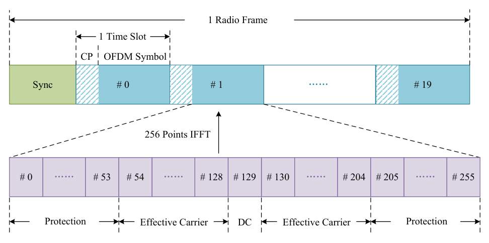
At the transmitter side, the transmitting bits are QPSK-modulated and IFFT-based OFDM modulated to obtain OFDM symbols in the time domain. After the CP is added to the corresponding OFDM symbol, the radio frame is transmitted by an USRP-RIO through a RF antenna whose center frequency is set to 2 GHz. At the receiver side, wireless signals are received by an USRP-RIO through a RF antenna. The receiver first conducts frame detection. After CP removal and FFT-based OFDM demodulation, the USRP-RIO performs least-square channel estimation. Finally, the results are stored into .csv files for future use.

The entire OTA test is divided into two phases. The first phase obtains samples in different scenarios with the help of the RaPro system shown in Fig. 14. The second phase employs the network trained under different training sets to verify the robustness of the TurboNet+ in real channels. We chose four different scenarios to evaluate our TurboNet+ in real environments.

1. $\bullet$

   Scenario 1: fixed indoor scenario. The receiver is 4 meters away from the transmitter in a room with windows, walls, and corridor around;

2. $\bullet$

   Scenario 2: an indoor scenario. Unlike Scenario 1, the antennas are 5 meters apart and are not facing each other;

3. $\bullet$

   Scenario 3: a changing indoor scenario. Unlike Scenario 2, pedestrians keep walking between the antennas;

4. $\bullet$

   Scenario 4: a changing indoor scenario. The only difference from Scenario 3 is that the antennas are 6 meters apart.

The measured BER is shown in Table III. From the Table III, the models trained in matched scenarios always achieve the best performance, thereby reflecting the TurboNet+’s strong ability to learn new scenarios. Moreover, the training samples obtained at a single transmitting power can help the TurboNet+ to achieve significant improvement over a wide range of transmitting power, a feature that is consistent with the simulation results. Table III shows that the model trained in Scenario 1 can achieve similar performance in new scenarios compared with the retrained model and this outcome indicates the TurboNet+’s strong robustness. Note that the model trained with samples generated by simulation under an AWGN channel can also achieve decent results in the real scenarios. Although the gain obtained cannot meet the above two models, a considerable improvement is achieved compared with the traditional max-log-MAP algorithm. In general, the TurboNet+ exhibits strong learning ability and robustness under real channels.

References

- [1] D. J. Costello and G. D. Forney, “Channel coding: The road to channel capacity,” Proc. of the IEEE, vol. 95, no. 6, pp. 1150–1177, Jul. 2007.
- [2] R. W. Hamming, “Error detecting and error correcting codes,” Bell Syst. Tech. J., vol. 29, pp. 147–160, Apr. 1950.
- [3] D. E. Muller, “Application of Boolean algebra to switching circuit design and to error detection,” IRE Trans. Electron. Comput., vol. EC–3, pp. 6–12, Sep. 1954.
- [4] R. C. Bose and D. K. Ray-Chaudhuri, “On a class of error-correcting binary group codes,” Inform. Contr., vol. 3, pp. 68–79, Mar. 1960.
- [5] I. S. Reed and G. Solomon, “Polynomial codes over certain finite fields,” J. SIAM, vol. 8, pp. 300–304, Jun. 1960.
- [6] P. Elias, “Coding for noisy channels,” IRE Conv. Rec., pt. 4, pp. 37–46, Mar. 1955.
- [7] C. Berrou, A. Glavieux, and P. Thitimajshima, “Near Shannon limit error-correcting coding and decoding: Turbo-codes,” in Proc. IEEE ICC, Geneva, Switzerland, May 1993, pp. 1064–1070.
- [8] R. G. Gallager, “Low-density parity-check codes,” IEEE Trans. Inf. Theory, vol. 8, no. 1, pp.21–28, Jan. 1962.
- [9] E. Arikan, “Channel polarization: A method for constructing capacity-achieving codes for symmetric binary-input memoryless channels,” IEEE Trans. Inf. Theory, vol. 55, no. 7, pp. 3051–3073, Jul. 2009.
- [10] T. J. O’ Shea and J. Hoydis, “An introduction to deep learning for the physical layer,” IEEE Trans. Cogn. Commun. Netw., vol. 3, no. 4, pp. 563–575, Dec. 2017.
- [11] T. Wang, C.-K. Wen, H. Wang, F. Gao, T. Jiang and S. Jin, “Deep learning for wireless physical layer: Opportunities and challenges,” China Commun., vol. 14, no. 11, pp. 92–111, Nov. 2017.
- [12] Z.-J. Qin, H. Ye, G. Y. Li, and B.-H. Juang, “Deep learning in physical layer communications,” IEEE Wireless Commun., vol. 26, no. 2, pp. 93–99, Apr. 2019.
- [13] T. J. O’ Shea, T. Roy, and T. C. Clancy, “Over-the-air deep learning based radio signal classification,” IEEE J. Sel. Top. Sign. Proces., vol. 12, no. 1, pp. 168–179, Jan. 2018.
- [14] H. He, C.-K. Wen, S. Jin, and G. Y. Li, “Model-driven deep learning for MIMO detection,” in IEEE. Trans. Signal Process., vol. 68, pp. 1702–1715, Feb. 2020, .
- [15] H. Ye, G. Y. Li, and B. H. Juang, “Power of deep learning for channel estimation and signal detection in OFDM systems,” IEEE Wireless Commun. Lett., vol. 7, no. 1, pp. 114–117, Feb. 2018.
- [16] X. Gao, S. Jin, C.-K. Wen, and G. Y. Li, “ComNet: Combination of deep learning and expert knowledge in OFDM receivers,” IEEE Commun. Lett., pp. 2627–2630, Dec. 2018.
- [17] J. Zhang, C.-K. Wen, S. Jin and G. Y. Li, “Artificial intelligence-aided receiver for a CP-free OFDM system: Design, simulation, and experimental test,” IEEE Access, vol. 7, pp. 58901–58914, May 2019.
- [18] C.-K. Wen, W. Shih, and S. Jin, “Deep learning for massive MIMO CSI feedback,” IEEE Wireless Commun. Lett., vol. 7, no. 5, pp. 748–751, Oct. 2018.
- [19] T. Wang, C.-K. Wen, S. Jin, and G. Y. Li, “Deep learning-based CSI feedback approach for time-varying massive MIMO channels,” IEEE Wireless Commun. Lett., vol. Early Access, pp. 1–10, Oct. 2018.
- [20] S. Dörner, S. Cammerer, J. Hoydis, and S. t. Brink, “Deep learning-based communication over the air,” IEEE J. Sel. Topics Signal Process., vol. 12, no. 1, pp. 132–143, Feb. 2018.
- [21] H. Ye, L. Liang, G. Y. Li, and B.-H. Juang, “Deep learning-based end-to-end wireless communication systems with conditional GANs as unknown channels,” in IEEE Trans. Wireless Commun., vol 19, no. 5, pp. 3133–3143, May 2020.
- [22] T. Gruber, S. Cammerer, J. Hoydis, and S. ten Brink, “On deep learning-based channel decoding,” in Proc. IEEE 51st ACISS., Mar. 2017, pp. 1–6.
- [23] X.-A. Wang and S. B. Wicker, “An artificial neural net Viterbi decoder,” IEEE Trans. Commun., vol. 44, no. 2, pp. 165–171, Feb. 1996.
- [24] H. Kim, Y. Jiang, R. B. Rana, S. Kannan, S. Oh, and P. Viswanath, “Communication algorithms via deep learning,” in ICLR 2018, Vancouver, Canada, Apr. 2018, pp. 1-17.
- [25] Z. Cao, H. Zhu, Y. Zhao, and D. Li, “Learning to denoise and decode: A novel residual neural network decoder for polar codes,” preprint, 2019. [Online]. Available: http://arxiv.org/abs/1908.00460.
- [26] Y. Jiang, S. Kannan, H. Kim, S. Oh, H. Asnani, and P. Viswanath, “Deepturbo: Deep turbo decoder,” in SPAWC 2019, Cannes, France, Jul. 2019, pp. 1-5.
- [27] E. Nachmani, Y. Be’ery, and D. Burshtein, “Learning to decode linear codes using deep learning,” in Proc. IEEE Annu. Allerton Conf. Commun., Control, and Computing, 2016, pp. 341–346.
- [28] L. Lugosch and W. J. Gross, “Neural offset min-sum decoding,” in Proc. 2017 IEEE ISIT, Jun. 2017, pp. 1361–1365.
- [29] E. Nachmani, E. Marciano, L. Lugosch, W. J. Gross, D. Burshtein, and Y. Be’ery, “Deep learning methods for improved decoding of linear codes,” IEEE J. Sel. Topics Signal Process., vol. 12, no. 1, pp. 119–131, Feb. 2018.
- [30] I. Be’ery, N. Raviv, T. Raviv, and Y. Be’ery, “Active learning decoding of linear codes,” preprint, 2019. [Online]. Available: http://arxiv.org/abs/1906.02778.
- [31] Y. He, J. Zhang, C.-K. Wen, and S. Jin, “A model-driven DNN decoder based on max-log-MAP algorithm for turbo code,” in Proc. IEEE APWCS, Singapore, Singapore, Aug. 2019, pp. 1–5.
- [32] 3rd Generation Partnership Project; Technical Specification; Evolved Universal Terrestrial Radio Access (E-UTRA); Multiplexing and Channel Coding (Release 9) 3GPP Organizational Partners TS 36.212, Rev. 8.3.0, May 2008.
- [33] L. Bahl, J. Cocke, F. Jelinek, and J. Raviv, “Optimal decoding of linear codes for minimizing symbol error rate,” IEEE Trans. Inf. Theory, vol. IT-20, no. 2, pp. 284–287, Mar. 1974.
- [34] S. Talakoub, L. Sabeti, B. Shahrrava, and M. Ahmadi, “An improved Max-Log-MAP algorithm for turbo decoding and turbo equalization,” IEEE Trans. Instrum. Meas., vol. 56, no. 3, pp. 1058–1063, Jun. 2007.
- [35] P. Robertson, P. Hoeher, and E. Villebrun, “Optimal and sub-optimal maximum a posteriori algorithms suitable for turbo decoding,” Eur. Trans. Telecommun., vol. 8, no. 2, pp. 119–125, Mar.–Apr. 1997.
- [36] J. A. Erfanian, S. Pasupathy, and G. Gulak, “Reduced complexity symbol detectors with parallel structures for ISI channels,” IEEE Trans. Commun., vol. 42, no. 2–4, pp. 1661–1671, Feb.–Apr. 1994.
- [37] D. P. Kingma and J. Ba, “Adam: A method for stochastic optimization,” preprint, 2014. [Online]. Available: http://arxiv.org/abs/1412.6980.
- [38] J. Vogt and A. Finger, “Improving the max-log-MAP turbo decoder,” Electron. Lett., vol. 36, no. 23, pp. 1937–1939, Nov. 2000.
- [39] P. Jiang, T. Wang, B. Han, X. Gao, J. Zhang, C.-K. Wen, S. Jin, and G. Y. Li, “Artificial intelligence-aided OFDM receiver: Design and experimental results,” preprint, 2018. [Online]. Available: http://arxiv.org/abs/1812.06638.
- [40] X. Yang, Z. Huang, B. Han, S. Zhang, C.-K. Wen, F. Gao, and S. Jin, “RaPro: A novel 5G rapid prototyping system architecture,” IEEE Wireless Commun. Lett., vol. 6, no. 3, pp. 362–365, Apr. 2017.