Subgradient method with feasible inexact projections for constrained convex optimization problems

A. A. Aguiar Thanks: Instituto de Matemática e Estatística, Universidade Federal de Goiás, CEP 74001-970 - Goiânia, GO, Brazil, E-mails: ademiraguia@gmail.com, orizon@ufg.br, lfprudente@ufg.br. The authors was supported in part by CNPq grants 305158/2014-7 and 302473/2017-3, FAPEG/PRONEM- 201710267000532 and CAPES. O. P. Ferreira ¹¹footnotemark: 1 L. F. Prudente ¹¹footnotemark: 1

Abstract

In this paper, we propose a new inexact version of the projected subgradient method to solve nondifferentiable constrained convex optimization problems. The method combine $\epsilon$ -subgradient method with a procedure to obtain a feasible inexact projection onto the constraint set. Asymptotic convergence results and iteration-complexity bounds for the sequence generated by the method employing the well known exogenous stepsizes, Polyak’s stepsizes, and dynamic stepsizes are stablished.

Keywords: Subgradient method, feasible inexact projection, constrained convex optimization.

AMS subject classification: 49J52, 49M15, 65H10, 90C30.

1 Introduction

The Subgradient method is one of the most interesting iterative method for solving nondifferentiable convex optimization problems, which has its origin and development in the 60’s, see [12, 33]. Since then, the subgradient method has attracted the attention of the scientific community working on optimization. One of the factors that explains this interest is its simplicity and ease of implementation. In particular, allowing a low cost of storage and ready exploitation of separability and sparsity. For these reasons, several variants of this method have emerged and properties of it have been discovered throughout the years, resulting in a wide literature on the subject; see, for exemple [1, 3, 4, 16, 20, 26] and the references therein.

The aim of this paper is to present an inexact version of the projected subgradient method, which consists in using an inexact projection instead of the exact one, for minimizing a convex function $f:\mathbb{R}^{n}\to\mathbb{R}$ onto a closed and convex subset $C$ of $\mathbb{R}^{n}$ . The proposed method, that we call Subgradient-InexP method, generates a sequence $\{x_{k}\}$ where each iteration consists of two stages. The first stage performs a step from the current iterate $x_{k}$ in the opposite direction of a $\epsilon$ -subgradient of $f$ at $x_{k}$ and the second inexactly projects the resulting vector onto the feasible set $C$ . From the theoretical point of view, considering methods that use inexact projections are particularly interesting for the following reasons. Even when the projection onto a convex set is an easy problem, iterative methods provide only approximated solutions with small errors, due to round-off errors in floating-point arithmetics. Therefore, the study of inexact methods gives theoretical support for real computational implementations of exact schemes. On the other hand, in general, one drawback of methods that use exact projections is having to solve a quadratic problem at each stage, which may substantially increasing the cost per iteration if the number of unknowns is large. In fact, it may not be justified to compute exact projection when the current iterate $x_{k}$ is far from the solution of the problem in consideration. Moreover, a procedure for computing a feasible inexact projection may present a low computation cost per iteration in comparison with one that computes the exact projection. Thus, it seems reasonable to consider versions of projected subgradient method that compute the projection only approximately. In order to present formally and analyze the Subgradient-InexP method, we use the concept of feasible inexact projection with relative error, which was appeared in [35] (see also[10]). It is worth noting that the concept of feasible inexact projection also accepts an exact projection when it is easy to obtain. For instance, the exact projections onto a box or a second order cone is very easy to obtain; see, respectively, [29, p. 520] and [14, Proposition 3.3]. A feasible inexact projection onto a polyhedral closed convex set can be obtained using quadratic programming methods that generate feasible iterates, such as feasible active set methods and interior point methods; see, for example, [17, 29, 34]. It is worth mentioning that, if the exact projection is used, then Subgradient-InexP method becomes the projected subgradient method considered in [1]. Several methods similar to the projected subgradient method have been studied in different papers, see [16, 23]. However, as far as we know, none of them use the concept of feasible inexact projection.

The main tool used in our analysis of Subgradient-InexP method is a version of the inequality obtained in [9, Lemma 1.1]; see also a variant of it in [25, Lemma 2.1]. By using this inequality, we establish asymptotic convergence results and iteration-complexity bounds for the sequence generated by our method employing the well known exogenous stepsizes, Polyak’s stepsizes, and dynamic stepsizes. We point out that these stepsizes have been discussed extensively in the related literature, including [1, 16, 24, 25, 26, 36], where many of our results were inspired. Let us describe the results in the present and their relationship with the literature on the subject. With respect to the exogenous stepsize we establish convergence results without any compactness assumption, existence of a solution, and the iteration-complexity bound, which are similar to the well known bound presented in [1, 25]. In particular, for $C=\mathbb{R}^{n}$ , the convergence results merge into the ones presented in [9] and the iteration-complexity bound into [27, Theorem 3.2.2]. The asymptotic convergence result and the iteration-complexity bound obtained using Polyak’s stepsizes are similar to the corespondent ones in [25, 28, 30] and [28], respectively. Regarding to the dynamic stepsize, we establish global convergence in objective values as address, for example, in [16, 25]. In [24, Proposition 2.15], the authors presented the rate of convergence for another variant of subgradient method, known as incremental subgradient algorithms. This study allowed us to estimate an iteraction-complexity bound for the dynamic stepsize.

The organization of the paper is as follows. In Section 2, we present some notation and basic results used in our presentation. In Section 3 we describe the Subgradient-InexP method with different choices for the stepsize. The main results of the present paper, including the converge theorems and iteration-complexity, are presented in Section 4. Some numerical experiments are provided in Section 5. We conclude the paper with some remarks in Section 6.

2 Notation and definitions

In this section, we present some notations, definitions, and results used throughout the paper. We are interested in

\min\{f(x):~x\in C\},

(1)

where $C$ is a closed and convex subset of $\mathbb{R}^{n}$ , $f:\mathbb{R}^{n}\to\mathbb{R}$ is a convex function. We denote by

f^{*}:=\inf_{x\in C}f(x),

(2)

its infimal value (possibly $-\infty$ ) and by $\Omega^{*}$ its solution set (possibly $\Omega^{*}=\varnothing$ ). The next concept will be useful in the analysis of the sequence generated by the subgradient method to solve (1).

Definition 1.

A sequence $\{y_{k}\}\subset\mathbb{R}^{n}$ is said to be quasi-Fejér convergent to a nonempty set $W\subset\mathbb{R}^{n}$ if, for every $w\in W$ , there exists a sequence $\{\delta_{k}\}\subset\mathbb{R}$ such that $\delta_{k}\geq 0$ , $\sum_{k=1}^{\infty}\delta_{k}<+\infty$ , and

\|y_{k+1}-w\|^{2}\leq\|y_{k}-w\|^{2}+\delta_{k},\qquad\forall~k=0,1,\ldots.

When, $\delta_{k}=0$ , for all $k=0,1,\ldots.$ , $\{y_{k}\}$ is called Fejér convergent to a set $W$ .

The main property of the quasi-Fejér convergent sequence is stated in the next result, and its proof can be found in [8].

Theorem 1.

Let $\{y_{k}\}$ be a sequence in $\mathbb{R}^{n}$ . If $\{y_{k}\}$ is quasi-Fejér convergent to a nomempty set $W\subset\mathbb{R}^{n}$ , then $\{y_{k}\}$ is bounded. If furthermore, a cluster point $y$ of $\{y_{k}\}$ belongs to $W$ , then $\lim_{k\rightarrow\infty}y_{k}=y$ .

To describe the method for solving the problem (1) we need to define, for each $\epsilon\geq 0$ , the $\epsilon$ -subdifferential $\partial_{\epsilon}f(x)$ of a convex function $f$ at $x\in{\mathbb{R}}^{n}$ ,

\partial_{\epsilon}f(x):=\{s\in{\mathbb{R}}^{n}:~f(y)\geq f(x)+\langle s,y-x\rangle-\epsilon,~\forall y\in{\mathbb{R}}^{n}\}.

(3)

We end this section by presenting important properties of the set $\epsilon$ -subdifferential of a convex function, which proofs follow by combining [5, Proposition 4.3.1(a)] and [18, Proposition 4.1.1, Proposition 4.1.2].

Proposition 2.

Let $f:\mathbb{R}^{n}\to\mathbb{R}$ be a convex function and $\epsilon\geq 0$ . The set $\partial_{\epsilon}f(x)$ is nonempty, convex, and compact. Moreover, if $B\subset\mathbb{R}^{n}$ is a bounded set, then there exists a real number $L>0$ such that $\|s\|<L$ , for all $s\in\cup_{x\in B}\partial_{\epsilon}f(x)$ . In addition, if $\{\epsilon_{k}\}$ is a bounded sequence of nonnegative real numbers, the sequence $\{x_{k}\}$ converges to $x\in\mathbb{R}^{n}$ , and $s_{k}\in\partial_{\epsilon_{k}}f(x_{k})$ for all $k$ , then the sequence $\{s_{k}\}$ is bounded.

3 Subgradient-InexP method

Next, we present the subgradient method with a feasible inexact projections, which will be called Subgradient-InexP method. We begin by presenting the concept of relative feasible inexact projection, which is a variation of those presented in [10, 35].

Definition 2.

Let $C\subset{\mathbb{R}}^{n}$ be a closed convex set and $\varphi_{\gamma,\theta,\lambda}:{\mathbb{R}}^{n}\times{\mathbb{R}}^{n}\times{\mathbb{R}}^{n}\to{\mathbb{R}}_{+}$ be a relative error tolerance function such that

\varphi_{\gamma,\theta,\lambda}(u,v,w)\leq\gamma\|v-u\|^{2}+\theta\|w-v\|^{2}+\lambda\|w-u\|^{2},\qquad\forall~u,v,w\in\mathbb{R}^{n},

(4)

where $\gamma,\theta,\lambda\geq 0$ are given forcing parameters. The feasible inexact projection mapping relative to $u\in C$ with relative error tolerance function $\varphi_{\gamma,\theta,\lambda}$ , denoted by ${\cal P}_{C}(\varphi_{\gamma,\theta,\lambda},u,\cdot):{\mathbb{R}}^{n}\rightrightarrows C$ is the set-valued mapping defined as follows

{\cal P}_{C}(\varphi_{\gamma,\theta,\lambda},u,v):=\left\{w\in C:~\left\langle v-w,z-w\right\rangle\leq\varphi_{\gamma,\theta,\lambda}(u,v,w),\quad\forall~z\in C\right\}.

(5)

Each point $w\in{\cal P}_{C}(\varphi_{\gamma,\theta,\lambda},u,v)$ is called a feasible inexact projection of $v$ onto $C$ relative to $u$ and with relative error tolerance function $\varphi_{\gamma,\theta,\lambda}$ .

In the following, we present some remarks about the definition of the feasible inexact projection mapping onto the convex set $C$ .

Remark 1.

Let $C\subset{\mathbb{R}}^{n}$ , $u\in C$ and $\varphi_{\gamma,\theta,\lambda}$ be as in Definition 2. Therefore, for all $v\in{\mathbb{R}}^{n}$ , it follows from (5) that ${\cal P}_{C}(0,u,v)$ is the exact projection of $u$ onto $C$ ; see [4, Proposition 2.1.3, p. 201]. Moreover, ${\cal P}_{C}(0,u,v)\in{\cal P}_{C}(\varphi_{\gamma,\theta,\lambda},u,v)$ concluding that ${\cal P}_{C}(\varphi_{\gamma,\theta,\lambda},u,v)\neq\varnothing$ , for all $u\in C$ and $v\in{\mathbb{R}}^{n}$ . Consequently, the set-valued mapping ${\cal P}_{C}(\varphi_{\gamma,\theta,\lambda},u,\cdot)$ is well-defined.

Next lemma is a variation of [11, Lemma 6]. It will play an important role in the remainder of this paper.

Lemma 3.

Let $v\in{\mathbb{R}}^{n}$ , $u\in C$ , $\gamma,\theta,\lambda\geq 0$ and $w\in{\cal P}_{C}(\varphi_{\gamma,\theta,\lambda},u,v)$ . Then, there holds

\|w-x\|^{2}\leq\|v-x\|^{2}+\frac{2\gamma+2\lambda}{1-2\lambda}\|v-u\|^{2},\qquad\forall~x\in C,

for all $\lambda,\theta\in[0,1/2)$ .

Proof.

Let $x\in C$ . First note that $\|w-x\|^{2}=\|v-x\|^{2}-\|w-v\|^{2}+2\langle v-w,x-w\rangle$ . Since $w\in{\cal P}_{C}(\varphi_{\gamma,\theta,\lambda},u,v)$ and $0\leq\theta<1/2$ , combining the last equality with (4) and (5) we obtain

	$\displaystyle\\|w-x\\|^{2}$	$\displaystyle\leq\\|v-x\\|^{2}-(1-2\theta)\\|v-w\\|^{2}+2\gamma\\|v-u\\|^{2}+2\lambda\\|w-u\\|^{2}$
		$\displaystyle\leq\\|v-x\\|^{2}+2\gamma\\|v-u\\|^{2}+2\lambda\\|w-u\\|^{2}.$		(6)

On the other hand, we also have

	$\displaystyle\\|w-u\\|^{2}$	$\displaystyle=\\|v-u\\|^{2}+\\|w-v\\|^{2}+2\langle v-w,u-v\rangle$
		$\displaystyle=\\|v-u\\|^{2}+\\|w-v\\|^{2}+2\langle v-w,u-w\rangle-2\\|w-v\\|^{2}$
		$\displaystyle=\\|v-u\\|^{2}-\\|w-v\\|^{2}+2\langle v-w,u-w\rangle.$

Thus, due to $w\in{\cal P}_{C}(\varphi_{\gamma,\theta,\lambda},u,v)$ and $u\in C$ , using (4), (5), $0\leq\theta<1/2$ and $0\leq\lambda<1/2$ , we have

\|w-u\|^{2}\leq\frac{1+2\gamma}{1-2\lambda}\|v-u\|^{2}-\frac{1-2\theta}{1-2\lambda}\|w-v\|^{2}\leq\frac{1+2\gamma}{1-2\lambda}\|v-u\|^{2}.

Therefore, combining the last inequality with (6), we obtain the desired inequality. ∎

The conceptual subgradient method with feasible inexact projections for solving the Problem (1) is formally defined as follows:

Step 0.

Let $\{\epsilon_{k}\}$ , $\{\theta_{k}\}$ , and $\{\lambda_{k}\}$ be sequences of nonnegative real numbers. Let $x_{0}\in C$ and set $k=0$ .

Step 1.

If $0\in\partial f(x_{k})$ , then stop. Otherwise, choose a non-null element $s_{k}\in\partial_{\epsilon_{k}}f(x_{k})$ , compute a stepsize $t_{k}>0$ , (to be specified later), and take the next iterate as any point such that

x_{k+1}\in{\cal P}_{C}\left(\varphi_{\gamma_{k},\theta_{k},\lambda_{k}},x_{k},x_{k}-t_{k}s_{k}\right).

Step 2.

Set $k\leftarrow k+1$ , and go to Step 1.

Algorithm 1 Subgradient-InexP method

Let us describe the main features of the subgradient-InexP method. Firstly, we check if the current iterate $x_{k}$ is a solution of Problem (1). If $x_{k}$ is not a a solution, then we choose a non-null element $s_{k}\in\partial_{\epsilon_{k}}f(x_{k})$ , compute a stepsize $t_{k}>0$ , and take the next iterate $x_{k+1}\in C$ as any feasible inexact projection of $x_{k}-t_{k}s_{k}$ onto $C$ relative to $x_{k}$ with error tolerance given by $\varphi_{\gamma_{k},\theta_{k},\lambda_{k}}(x_{k},x_{k}-t_{k}s_{k},x_{k+1})$ , i.e., $x_{k+1}\in{\cal P}_{C}\left(\varphi_{\gamma_{k},\theta_{k},\lambda_{k}},x_{k},x_{k}-t_{k}s_{k}\right)$ . We remark that if $\varphi_{\gamma_{k},\theta_{k},\lambda_{k}}\equiv~0$ , then ${\cal P}_{C}\left(0,x_{k},x_{k}-t_{k}s_{k}\right)$ is the exact projection of $x_{k}-t_{k}s_{k}$ onto $C$ , and Algorithm 1 amounts to the projected subgradient method studied in [1]. Among the several possible choices that appeared in literature on subject, see for example [4, 25, 33], we studied three well known strategies, beginning with exogenous stepsize.

Rule 1 (Exogenous stepsize).

Let $\mu\geq 0$ . Take exogenous sequences $\{\alpha_{k}\}$ and $\{\epsilon_{k}\}$ of nonnegative real numbers satisfying the following conditions: the sequence $\{\epsilon_{k}\}$ is nonincreasing and

\sum_{k=0}^{\infty}\alpha_{k}=+\infty,\qquad\qquad\sum_{k=0}^{\infty}\alpha_{k}^{2}<+\infty,\qquad\qquad\epsilon_{k}\leq\mu\alpha_{k},\qquad\qquad~k=0,1,\ldots.

(7)

Given $s_{k}\in\partial_{\epsilon_{k}}f(x_{k})$ , define the stepsize $t_{k}$ as the following nonnegative real number

t_{k}:=\frac{\alpha_{k}}{\eta_{k}},\qquad\qquad\eta_{k}:=\max\left\{1,\|s_{k}\|\right\},\qquad\qquad~k=0,1,\ldots.

(8)

The stepsize in Rule 1 is one the most popular. It have been used in several paper for analyzing subgradient method; see for example, [1, 9, 24, 25, 36].

From now on we assume that there exist $0\leq\bar{\theta}<1/2$ and $0\leq\bar{\lambda}<1/2$ , such that $\{\theta_{k}\}\subset[0,{\bar{\theta}})$ , $\{\gamma_{k}\}\subset[0,{\bar{\gamma}})$ and $\{\lambda_{k}\}\subset[0,{\bar{\lambda}})$ . For future references define

\nu:=\frac{1+2{\bar{\gamma}}}{1-2{\bar{\lambda}}}>0.

(9)

To define the next stepsize, we need to known the optimum value $f^{*}$ given in (2). In [31, p.142], is present some examples of problems for which the optimum value are known. The statement of the Polyak’s stepsize is as follows.

Rule 2 (Polyak’s stepsize).

Assume that $\Omega^{*}\neq\varnothing$ and the optimal value $f^{*}>-\infty$ is known. Let $\mu\geq 0$ , $\underline{\beta}>0$ , ${\bar{\beta}}>0$ and take exogenous sequences $\{\beta_{k}\}$ and $\{\epsilon_{k}\}$ of real numbers satisfying the following conditions: the sequence $\{\epsilon_{k}\}$ is nonincreasing and

0<\underline{\beta}\leq\beta_{k}\leq\bar{\beta}<\frac{1}{2\mu+\nu},\qquad\qquad 0<\epsilon_{k}\leq\mu\beta_{k}[f(x_{k})-f^{*}],\quad\qquad~k=0,1,\ldots.

(10)

Given $s_{k}\in\partial_{\epsilon_{k}}f(x_{k})$ , $s_{k}\neq 0$ , define the stepsize $t_{k}$ as the following nonnegative real number

t_{k}=\beta_{k}\frac{f(x_{k})-f^{*}}{\left\|s_{k}\right\|^{2}},\qquad\qquad~k=0,1,\ldots.

(11)

The stepsize in Rule 2 was introduced in [30] and has been used in several papers, including the ones [24, 25, 36]. In general, in practical problems the optimum value (2) is not known. In this case, we may modify the stepsize (11) by replacing the optimum value (2) with a suitable estimate in each iteration. This leads to the dynamic stepsize rule as follows.

Rule 3 (Dynamic stepsize).

Let $\mu\geq 0$ , $\underline{\beta}>0$ , ${\bar{\beta}}>0$ , and take exogenous sequences $\{\beta_{k}\}$ and $\{\epsilon_{k}\}$ of real numbers satisfying the following conditions: the sequence $\{\epsilon_{k}\}$ is nonincreasing and

0<\underline{\beta}\leq\beta_{k}\leq\bar{\beta}<\frac{2}{2\mu+\nu},\qquad\qquad 0<\epsilon_{k}\leq\mu\beta_{k}[f(x_{k})-f_{k}^{lev}],\quad\qquad~k=0,1,\ldots,

(12)

where $f_{k}^{lev}$ will be specified later (see Section 4.3). Given $s_{k}\in\partial_{\epsilon_{k}}f(x_{k})$ such that $s_{k}\neq 0$ , define the stepsize $t_{k}$ as the following nonnegative real number

t_{k}=\frac{\tilde{t}_{k}}{\left\|s_{k}\right\|},\qquad\qquad\tilde{t}_{k}=\beta_{k}\frac{f(x_{k})-f_{k}^{lev}}{\left\|s_{k}\right\|},\qquad\qquad~k=0,1,\ldots.

(13)

The dynamic stepsize in Rule 3 is based on the ideas of [7]; see also [16]. This rule has been used in several papers, see for example [25, 26, 36].

From now on we assume that the sequence $\{x_{k}\}$ is generated by Algorithm 1, with one of the three above strategies for choosing the stepsize, is infinite.

4 Analysis of the subgradient-InexP method

In the following, we state and prove our first result to analyze the sequence $\{x_{k}\}$ generated by Algorithm 1. The obtained inequality in next lemma is its counterpart for unconstrained optimization provided in [9, Lemma 1.1)]. As we shall see, this inequality will be the main tool in our asymptotic convergence analysis, as well as in the iteration-complexity analysis.

Lemma 4.

Let $\nu>0$ be as defined (9). For all $x\in C$ , the following inequality holds

\|x_{k+1}-x\|^{2}\leq\|x_{k}-x\|^{2}+\nu t_{k}^{2}\|s_{k}\|^{2}-2t_{k}\left[f(x_{k})-f(x)-\epsilon_{k}\right],\qquad k=0,1,\ldots.

(14)

Proof.

Let $x\in C$ . To simply the notations we set $z_{k}:=x_{k}-t_{k}s_{k}$ . Due to $x_{k+1}\in{\cal P}_{C}\left(\varphi_{\gamma_{k},\theta_{k},\lambda_{k}},x_{k},z_{k}\right)$ and $x_{k}\in C$ , we apply Lemma 3 with $w=x_{k+1}$ , $v=z_{k}$ , $u=x_{k}$ , and $\varphi_{\gamma,\theta,\lambda}=\varphi_{\gamma_{k},\theta_{k},\lambda_{k}}$ to conclude

\|x_{k+1}-x\|^{2}\leq\|z_{k}-x\|^{2}+\frac{2\gamma_{k}+2\lambda_{k}}{1-2\lambda_{k}}t_{k}^{2}\|s_{k}\|^{2}.

(15)

On the other hand, due to $z_{k}=x_{k}-t_{k}s_{k}$ , after some algebraic manipulations, we obtain

\|z_{k}-x\|^{2}=\|x_{k}-x\|^{2}+t_{k}^{2}\|s_{k}\|^{2}+2t_{k}\langle s_{k},x-x_{k}\rangle.

Since $s_{k}\in\partial_{\epsilon_{k}}f(x_{k})$ , the definition (3) implies that $\langle s_{k},z-x_{k}\rangle\leq f(z)-f(x_{k})+\epsilon_{k}$ . Thus,

\|z_{k}-x\|^{2}\leq\|x_{k}-x\|^{2}+t_{k}^{2}\|s_{k}\|^{2}+2t_{k}\left[f(x)-f(x_{k})+\epsilon_{k}\right].

Therefore, combining last inequality with (15) we conclude that

	$\displaystyle\\|x_{k+1}-x\\|^{2}$	$\displaystyle\leq\\|x_{k}-x\\|^{2}+t_{k}^{2}\\|s_{k}\\|^{2}+2t_{k}\left[f(x)-f(x_{k})+\epsilon_{k}\right]+\frac{2\gamma_{k}+2\lambda_{k}}{1-2\lambda_{k}}t_{k}^{2}\\|s_{k}\\|^{2}$
		$\displaystyle=\\|x_{k}-x\\|^{2}+\frac{1+2\gamma_{k}}{1-2\lambda_{k}}t_{k}^{2}\\|s_{k}\\|^{2}-2t_{k}\left[f(x_{k})-f(x)-\epsilon_{k}\right].$

Considering that $0\leq\lambda_{k}<\bar{\lambda}<1/2$ and $0\leq\gamma_{k}<\bar{\gamma}$ , and using (9), we obtain (14). ∎

4.1 Analysis of the subgradient-InexP method with exogenous stepsize

In this section we will analyze the subgradient-InexP method with stepsizes satisfying Rule 1. For that, throughout this section we assume also that $\{x_{k}\}$ is a sequence generated by Algorithm 1 with the stepsize given by Rule 1 and, define

\rho:=\nu+2\mu>0.

(16)

First of all, note that under the above assumptions, Lemma 4 becomes as follows.

Lemma 5.

Let $\rho>0$ be as in (16). For all $x\in C$ , the following inequality holds

\|x_{k+1}-x\|^{2}\leq\|x_{k}-x\|^{2}+\rho\alpha_{k}^{2}-2\frac{\alpha_{k}}{\eta_{k}}\left[f(x_{k})-f(x)\right],\qquad k=0,1,\ldots.

Proof.

The definition of $t_{k}$ in (8) implies $t_{k}\leq\alpha_{k}$ , which combined with the last inequality in (7) yields $2t_{k}\epsilon_{k}\leq 2\mu\alpha_{k}^{2}$ . Moreover, (8) also implies that $t_{k}^{2}\|s_{k}\|^{2}\leq\alpha_{k}^{2}$ . Therefore, using (16), the desired inequality follows directly from (14). ∎

To proceed with the analysis of Algorithm 1, we also need the following auxiliary set

\Omega:=\left\{x\in C:~f(x)\leq\inf_{k}f(x_{k})\right\}.

(17)

It is worth mentioning that, in principle, set $\Omega$ can be empty and, in such case, $f^{*}=-\infty$ . In the next lemma we analyze the behavior of the sequence $\{x_{k}\}$ under the hypothesis that $\Omega\neq\varnothing$ .

Lemma 6.

If $\Omega\neq\varnothing$ , then $\{x_{k}\}$ is quasi-Féjer convergent to $\Omega$ . Consequently, $\{x_{k}\}$ is bounded.

Proof.

Since $\Omega\neq\varnothing$ , take $x\in\Omega$ . Thus, by using the definition of $\Omega$ in (17) and Lemma 5, we conclude that $\|x_{k+1}-x\|^{2}\leq\|x_{k}-x\|^{2}+\rho\alpha_{k}^{2}$ , for all $k=0,1,\ldots$ . Hence, using the first inequality in (7), the first statement of the lemma follows from Definition 1. The second statement of the lemma follows from the first part of Theorem 1. ∎

Now, we are ready to prove the main result of this section, which refers to the asymptotic convergence of $\{x_{k}\}$ . We remark that in the first part of the next theorem we do not assume neither $\Omega^{*}\neq\varnothing$ nor that $f^{*}$ is finite.

Theorem 7.

The following equality holds

\liminf_{k}f(x_{k})=f^{*}.

(18)

In addition, if $\Omega^{*}\neq\varnothing$ then the sequence $\{x_{k}\}$ converges to a point $x_{*}\in\Omega^{*}$ .

Proof.

Assume by contradiction that $\liminf_{k}f(x_{k})>f^{*}$ . In this case, we have $\Omega\neq\varnothing$ . Consequently by Lemma 6, we conclude that $\{x_{k}\}$ is bounded. Letting $x\in\Omega$ , there exist $\tau>0$ and $k_{0}\in\mathbb{N}$ such that $f(x)<f(x_{k})-\tau,$ for all $k\geq k_{0}$ . Hence, using Lemma 5, we have

\|x_{k+1}-x\|^{2}\leq\|x_{k}-x\|^{2}+\rho\alpha_{k}^{2}-2\frac{\alpha_{k}}{\eta_{k}}\tau,\qquad k=k_{0},k_{0}+1,\dots.

(19)

On the other hand, it follows from (7) that the sequence $\left\{\epsilon_{k}\right\}$ is bounded. Thus, considering that $\{x_{k}\}$ is bounded, Proposition 2 implies that $\{s_{k}\}$ is also bounded. Let $c>0$ be such that $\|s_{k}\|\leq c$ , for all $k\geq 0$ . Hence, using second equality in (8), we have $\eta_{k}=\max\left\{1,\|s_{k}\|\right\}\leq\max\left\{1,c\right\}=:\varGamma$ . Thus, letting $\ell\in\mathbb{N}$ and using (19), we conclude that

\frac{2\tau}{\varGamma}\sum_{j=k_{0}}^{\ell+k_{0}}\alpha_{j}\leq\|x_{k_{0}}-x\|^{2}-\|x_{k_{0}+\ell+1}-x\|+\rho\sum_{j=k_{0}}^{\ell+k_{0}}\alpha^{2}_{j}\leq\|x_{k_{0}}-x\|^{2}+\rho\sum_{j=k_{0}}^{\ell+k_{0}}\alpha^{2}_{j}.

Since the last inequality holds for all $\ell\in\mathbb{N}$ then, by using the first two conditions on $\{\alpha_{k}\}$ in (7), we have a contraction. Therefore, (18) holds. For proving the last statement, let us assume that $\Omega^{*}\neq\varnothing$ . In this case, we also have $\Omega\neq\varnothing$ and, from Lemma 6, the sequence $\{x_{k}\}$ is bounded and quasi-Féjer convergent to $\Omega$ . The equality (18) implies that $\{f(x_{k})\}$ has a decreasing monotonous subsequence $\{f(x_{k_{j}})\}$ such that $\lim_{j\rightarrow\infty}f(x_{k_{j}})=f^{*}.$ Without lose of generality, we can assume that $\{f(x_{k})\}$ is decreasing, is monotonous, and converges to $f^{*}$ . Being bounded, the sequence $\{x_{k}\}$ has a convergent subsequence $\{x_{k_{\ell}}\}$ . Let us say that $\lim_{\ell\rightarrow\infty}x_{k_{\ell}}=x_{*},$ which by the continuity of $f$ implies $f(x_{*})=\lim_{\ell\rightarrow\infty}f(x_{k_{\ell}})=f^{*},$ and then $x_{*}\in\Omega^{*}$ . Hence, $\{x_{k}\}$ has an cluster point $x_{*}\in\Omega$ , and due to $\{x_{k}\}$ be quasi-Féjer convergent to $\Omega$ , Theorem 1 implies that $\{x_{k}\}$ converges to $x_{*}$ . ∎

Next theorem presents an iteration-complexity bound; similar bound can be found in [27, Theorem 3.2.2].

Theorem 8.

Assume that the sequence $\{x_{k}\}$ converges to a point $x_{*}\in\Omega^{*}$ . Then, for every $N\in\mathbb{N}$ , the following inequality holds

\min\{f(x_{k})-f^{*}:~\,k=0,1,\ldots,N\}\leq\varGamma\frac{\|x_{0}-x_{*}\|^{2}+\rho\sum_{k=0}^{N}\alpha_{k}^{2}}{2\sum_{k=0}^{N}\alpha_{k}}.

Proof.

Since $\left\{\epsilon_{k}\right\}$ and $\left\{x_{k}\right\}$ are bounded sequences, then using Proposition 2, it follows that $\left\{s_{k}\right\}$ is also bounded, i.e. there exists $c>0$ such that $\|s_{k}\|\leq c$ , for all $k\geq 0$ . Therefore, using the definition of $\eta_{k}$ in (8), we have $\eta_{k}=\max\left\{1,\|s_{k}\|\right\}\leq\max\left\{1,c\right\}=:\varGamma$ . Now, applying Lemma 5 with $x=x_{*}$ and due to $f^{*}=f(x_{*})$ , we obtain

\frac{2\alpha_{k}}{\varGamma}[f(x_{k})-f^{*}]\leq\|x_{k}-x_{*}\|^{2}-\|x_{k+1}-x_{*}\|^{2}+\rho\alpha_{k}^{2},\qquad k=0,1,\ldots.

Hence, performing the sum of the above inequality for $k=0,1,\ldots,N,$ we have

\frac{2}{\varGamma}\sum_{k=0}^{N}\alpha_{k}[f(x_{k})-f^{*}]\leq\|x_{0}-x_{*}\|^{2}-\|x_{N+1}-x_{*}\|^{2}+\rho\sum_{k=0}^{N}\alpha_{k}^{2}.

Therefore,

\frac{2}{\varGamma}\,\min\left\{f(x_{k})-f^{*}:~\,k=0,1,\ldots,N\right\}\sum_{k=0}^{N}\alpha_{k}\leq\|x_{0}-x_{*}\|^{2}+\rho\sum_{k=0}^{N}\alpha_{k}^{2},

which is equivalent to the desired inequality. ∎

4.2 Analysis of the subgradient-InexP method with Polyak’s stepsize rule

In this section we will analyze the subgradient-InexP method with Polyak’s step sizes. Throughout this section, we assume also that $\Omega^{*}\neq\varnothing$ and $\{x_{k}\}$ is a sequence generated by Algorithm 1 with the stepsize given by Rule 2.

Lemma 9.

Let $x\in\Omega^{*}$ . Then, the following inequality holds

\|x_{k+1}-x\|^{2}\leq\|x_{k}-x\|^{2}-\underline{\beta}\frac{\left[f(x_{k})-f^{*}\right]^{2}}{\|s_{k}\|^{2}},\qquad\qquad k=0,1,\ldots.

(20)

Proof.

Considering that $x\in\Omega^{*}$ we have $f^{*}=f(x)$ . The combination of (10) with (11) implies $2t_{k}\epsilon_{k}\leq 2\mu\beta_{k}^{2}[f(x_{k})-f^{*}]^{2}/\|s_{k}\|^{2}$ . Moreover, (11) also implies that $t_{k}^{2}\|s_{k}\|^{2}=\beta_{k}^{2}[f(x_{k})-f^{*}]^{2}/\|s_{k}\|^{2}$ . Thus, we conclude form (14) that

\|x_{k+1}-x\|^{2}\leq\|x_{k}-x\|^{2}-\left(2-\nu\beta_{k}-2\mu\beta_{k}\right)\beta_{k}\frac{\left[f(x_{k})-f^{*}\right]^{2}}{\|s_{k}\|^{2}},\qquad k=0,1,\ldots.

(21)

On the other hand, (10) gives us $\beta_{k}<1/(2\mu+\nu)$ , which is equivalent to $2-\nu\beta_{k}-2\mu\beta_{k}>1$ . Therefore, since (10) also gives $\underline{\beta}\leq\beta_{k}$ , we conclude that (21) implies (20). ∎

In the following theorem we present our main result about the asymptotic convergence of $\{x_{k}\}$ . It has as correspondent result in [30, Theorem 1]; see also [25].

Theorem 10.

The sequence $\{x_{k}\}$ converges to a point $x_{*}\in\Omega^{*}$ .

Proof.

Let $x\in\Omega^{*}$ . Then, Lemma 9 implies $\|x_{k+1}-x\|^{2}\leq\|x_{k}-x\|^{2}$ , for all $k=0,1,\ldots$ . Thus, $\{x_{k}\}$ is Fejér convergent to $\Omega^{*}$ . Since $\Omega^{*}\neq\varnothing$ , Theorem 1 implies that $\{x_{k}\}$ is bounded. By using Proposition 2, we conclude that there exists $c>0$ such that $\left\|s_{k}\right\|\leq c$ , for $k=0,1,\ldots$ . Then, from (20), after some algebra, we have

\left[f(x_{k})-f^{*}\right]^{2}\leq\frac{c^{2}}{\underline{\beta}}\left(\|x_{k}-x\|^{2}-\|x_{k+1}-x\|^{2}\right),\qquad\qquad k=0,1,\ldots.

Thus, performing the sum of the this inequality for $j=0,1,\ldots,\ell$ , we obtain

\sum_{j=0}^{\ell}\left[f(x_{j})-f^{*}\right]^{2}\leq\frac{c^{2}}{\underline{\beta}}\left(\|x_{0}-x\|^{2}-\|x_{\ell+1}-x\|^{2}\right)\leq\frac{c^{2}}{\underline{\beta}}\|x_{0}-x\|^{2}.

Considering that this inequality holds for all $\ell\in\mathbb{N}$ , we conclude that $\lim_{k\to+\infty}f(x_{k})=f^{*}$ . Let $x_{*}$ be a cluster point of $\{x_{k}\}$ and $\{x_{k_{j}}\}$ a subsequence of $\{x_{k}\}$ such that $\lim_{j\to+\infty}x_{k_{j}}=x_{*}$ . Since $f$ is continuous, we have $f(x_{*})=\lim_{j\to+\infty}f(x_{k_{j}})=f^{*}$ . Therefore, $x_{*}\in\Omega^{*}$ . Since $\{x_{k}\}$ is quasi-Fejér convergent to a set $\Omega^{*}$ , it follows from Theorem 1 that $\{x_{k}\}$ converges $x_{*}$ . ∎

The next result presents an iteration-complexity bound, which is a version of [28, Theorem 1].

Theorem 11.

Assume that the sequence $\{x_{k}\}$ converges to a point $x_{*}\in\Omega^{*}$ . Then, for every $N\in\mathbb{N}$ , the following inequality holds

\min\{f(x_{k})-f^{*}:~\,k=0,1,\ldots,N\}\leq\frac{c}{\sqrt{\underline{\beta}(N+1)}}\|x_{0}-x_{*}\|,

where $c\geq\max\{\|s_{k}\|:~k=0,1,\ldots\}$ .

Proof.

Applying Lemma 9 with $x=x_{*}$ , where $f^{*}=f(x_{*})$ , we obtain

\underline{\beta}\frac{\left[f(x_{k})-f^{*}\right]^{2}}{\|s_{k}\|^{2}}\leq\|x_{k}-x_{*}\|^{2}-\|x_{k+1}-x_{*}\|^{2},\qquad\qquad k=0,1,\ldots.

Performing the sum of the above inequality for $k=0,1,\ldots,N,$ we conclude that

\sum_{k=0}^{N}\frac{\left[f(x_{k})-f^{*}\right]^{2}}{\|s_{k}\|^{2}}\leq\frac{1}{\underline{\beta}}\|x_{0}-x_{*}\|^{2}.

Since $\{x_{k}\}$ is bounded, by using Proposition 2, we conclude that there exists $c>0$ such that $\left\|s_{k}\right\|\leq c$ , for $k=0,1,\ldots$ . Thus, we have

\sum_{k=0}^{N}\left[f(x_{k})-f^{*}\right]^{2}\leq\frac{c^{2}}{\underline{\beta}}\|x_{0}-x_{*}\|^{2}.

Therefore,

(N+1)\min\{\left[f(x_{k})-f^{*}\right]^{2}:~\,k=0,1,\ldots,N\}\leq\frac{c^{2}}{\underline{\beta}}\|x_{0}-x_{*}\|^{2},

which is equivalent to the desired inequality. ∎

4.3 Analysis of the subgradient-InexP method with dynamic stepsize

Next we consider the Subgradient-InexP method employing the dynamic stepsize Rule 3, which guarantees that $\{f_{k}^{lev}\}$ converges to the optimum value $f^{*}$ . In the following we present formally the algorithm which compute $f_{k}^{lev}$ . This scheme was introduced in [7]; see also [16].

Step 0.: Select $x_{0}\in C,\delta_{0}>0$ , and $R>0$ . Set $k=0,\sigma_{0}=0,f_{-1}^{rec}=\infty,\ell=0,k(\ell)=0$ .
Step 1.: If $f(x_{k})<f_{k-1}^{rec},$ set $f_{k}^{rec}=f(x_{k})$ and $x_{k}^{rec}=x_{k},$ else set $f_{k}^{rec}=f_{k-1}^{rec}$ and $x_{k}^{rec}=x_{k-1}^{rec}$
Step 2.: If $0\in\partial f(x_{k})$ , then stop.
Step 3.: If $f(x_{k})\leq f_{k(\ell)}^{rec}-\frac{1}{2}\delta_{\ell}$ , set $k(\ell+1)=k,\sigma_{k}=0,\delta_{\ell+1}=\delta_{\ell}$ , replace $\ell$ by $\ell+1,$ and go to Step 5.
Step 4.: If $\sigma_{k}>R$ , set $k(\ell+1)=k,\sigma_{k}=0,\delta_{\ell+1}=\frac{1}{2}\delta_{\ell}$ , $x_{k}=x_{k}^{rec}$ , and $\ell\leftarrow\ell+1$ .
Step 5.: Set $f_{k}^{lev}:=f_{k(\ell)}^{rec}-\delta_{\ell}$ . Select $\beta_{k}\in[\underline{\beta},\bar{\beta}]$ and calculate $x_{k+1}$ via Algorithm 1 with the stepsize given by Rule 3.
Step 6.: Set $\sigma_{k+1}:=\sigma_{k}+\tilde{t}_{k}$ , $k\leftarrow k+1$ , and go to Step 1.

Algorithm 2 Subgradient-InexP employing the dynamic stepsize rule (SInexPD)

Following [16, 24, 25, 36], we describe the main features of the Subgradient-InexP method.

Remark 2.

Note that in Step 1, $f_{k}^{rec}$ keeps the record of the smallest functional value attained by the iterates generated so far, i.e., $f_{k}^{rec}:=\min\{f(x_{j}):~j=0,\ldots,k\}$ . Splitting the iterations into groups

K_{\ell}:=\{k(\ell),k(\ell)+1,\ldots,k(\ell+1)-1\},\quad\ell=0,1,\dots,

Algorithm 2 uses the same target level $f_{k}^{lev}=f_{k(\ell)}^{rec}-\delta_{\ell}$ , for $k\in K_{\ell}$ . Also, note that the target level is update only if sufficient descent or oscillation is detected (Step 3 or Step 4, respectively). Whenever $\sigma_{k}$ exceeds the upper bound $R$ , the parameter $\delta_{\ell}$ is decreased, which increases the target level $f_{k}^{lev}$ .

From now on, we assume that Algorithm 2 generates an infinite sequence. In the next theorem we present the result about the asymptotic convergence of the sequence $\{x_{k}\}$ . It is the versions of [16, Theorem 1] and [25, Proposition 2.7] by using inexact projections.

Theorem 12.

There holds $\inf_{k\geq 0}f(x_{k})=f^{*}$ .

Proof.

Since $x_{k}\in C$ and $x_{k+1}\in{\cal P}_{C}\left(\varphi_{\gamma_{k},\theta_{k},\lambda_{k}},x_{k},x_{k}-t_{k}s_{k}\right)$ , by the first equality in (13) and applying Lemma 3 with $w=x_{k+1}$ , $v=x_{k}-t_{k}s_{k}$ , $x=x_{k}$ , $u=x_{k}$ , and $\varphi_{\gamma,\theta,\lambda}=\varphi_{\gamma_{k},\theta_{k},\lambda_{k}}$ , we conclude that

\|x_{k+1}-x_{k}\|\leq\sqrt{\frac{1+2\bar{\gamma}}{1-2\bar{\lambda}}}\,\,t_{k}\|s_{k}\|\leq\sqrt{\frac{1+2\bar{\gamma}}{1-2\bar{\lambda}}}\,\,\tilde{t}_{k},\qquad k=0,1,\ldots.

We claim that the index $\ell$ goes to $+\infty$ and either $\inf_{k\geq 0}f(x_{k})=-\infty$ or $\lim_{l\to\infty}\delta_{\ell}=0$ . Indeed, assume that $\ell$ takes only a finite number of values, i.e., $\ell<\infty$ . Since $\sigma_{k}+\tilde{t}_{k}=\sigma_{k+1}\leq R$ , for all $k\geq k(\ell)$ , then we conclude that

\|x_{k}-x_{k(\ell)}\|\leq\sum_{j=k(\ell)}^{k}\|x_{j+1}-x_{j}\|\leq\sqrt{\frac{1+2\bar{\gamma}}{1-2\bar{\lambda}}}\sum_{j=k(\ell)}^{k}\tilde{t}_{j}=\sqrt{\frac{1+2\bar{\gamma}}{1-2\bar{\lambda}}}\,\,\sigma_{k+1}\leq\sqrt{\frac{1+2\bar{\gamma}}{1-2\bar{\lambda}}}\,\,R.

(22)

Hence, $\{x_{k}\}$ is bounded. Besides, from the last condition in (12), the sequence $\{\epsilon_{k}\}$ is bounded and, by using Proposition 2, $\{s_{k}\}$ is also bounded. Moreover, by (22) we also conclude $\sum_{j=k(\ell)}^{+\infty}\tilde{t}_{j}<+\infty$ , which implies $\lim_{k\to\infty}\tilde{t}_{k}=0$ . Thus, due to $\beta_{k}\in[\underline{\beta},\bar{\beta}]$ , it follows from second equality in (13) that

\lim_{k\to\infty}[f(x_{k})-f_{k}^{lev}]=0.

(23)

On the other hand, Steps 3 and 5 of Algorithm 2 yield

f(x_{k})>f_{k(\ell)}^{rec}-\frac{1}{2}\delta_{\ell}=f_{k}^{lev}+\delta_{\ell}-\frac{1}{2}\delta_{\ell}=f_{k}^{lev}+\frac{1}{2}\delta_{\ell}\qquad\quad k=k(\ell),k(\ell)+1,\ldots,

contradicting (23). Therefore, $\ell$ goes to $+\infty$ . Now, suppose that $\lim_{\ell\to\infty}\delta_{\ell}=\delta>0$ . Then, from Steps 3 and 4 of Algorithm 2, it follows that for all $\ell$ large enough, we have $\delta_{\ell}=\delta$ and $f_{k(\ell+1)}^{rec}\leq f_{k(\ell)}^{rec}-\frac{1}{2}\delta,$ implying that $\displaystyle\inf_{k\geq 0}f(x_{k})=-\infty$ , which concludes the claim. If $\lim_{\ell\to\infty}\delta_{\ell}>0$ then, according to above claim, we have $\inf_{k\geq 0}f(x_{k})=-\infty$ , obtain the desired result. Now, we assume by contradiction that $\lim_{\ell\to\infty}\delta_{\ell}=0$ and $\inf_{k\geq 0}f(x_{k})>f^{*}$ . Thus, it follows from Remark 2 that $\inf_{k\geq 0}f_{k}^{rec}=\inf_{k\geq 0}f(x_{k})$ . Hence, we conclude that $\inf_{k\geq 0}f_{k}^{rec}>f^{*}$ . In this case, by using the definition of $\{f_{k}^{lev}\}$ in Step 5 and taking into account that $\lim_{\ell\to\infty}\delta_{\ell}=0$ , we conclude that

\displaystyle\inf_{k\geq 0}f_{k}^{lev}=\displaystyle\inf_{\ell\geq 0}(f_{k(\ell)}^{rec}-\delta_{\ell})=\displaystyle\inf_{\ell\geq 0}f_{k(\ell)}^{rec}>f^{*}.

Therefore, there exist $\bar{\delta}>0$ , ${\bar{x}}\in C$ and $\bar{k}\in\mathbb{N}$ such that

f_{k}^{lev}-f({\bar{x}})\geq\bar{\delta},\qquad k=\bar{k},\bar{k}+1,\ldots.

(24)

Hence, by using the definition of $\tilde{t}_{k}$ in (13), it follows from (24) that

\tilde{t}_{k}=\beta_{k}\frac{f(x_{k})-f_{k}^{lev}}{\left\|s_{k}\right\|}<\bar{\beta}\frac{f(x_{k})-f({\bar{x}})-\bar{\delta}}{\left\|s_{k}\right\|},\qquad k=\bar{k},\bar{k}+1,\ldots.

(25)

Now, applying Lemma 4 with $x={\bar{x}}$ and then using (11) and (13), we obtain

\|x_{k+1}-{\bar{x}}\|^{2}\leq\|x_{k}-{\bar{x}}\|^{2}+\tilde{t}_{k}\left(\nu\tilde{t}_{k}-\frac{2}{\|s_{k}\|}\left[f(x_{k})-f({\bar{x}})-\epsilon_{k}\right]\right),\qquad k=\bar{k},\bar{k}+1,\ldots.

Thus, the combination of the last inequality with (24), (25), and the last inequality in (12) yields

\|x_{k+1}-{\bar{x}}\|^{2}\leq\|x_{k}-{\bar{x}}\|^{2}+\frac{\tilde{t}_{k}}{\|s_{k}\|}\bigg(\left[(2\mu+\nu)\bar{\beta}-2\right]\left[f(x_{k})-f({\bar{x}})\right]-\left(2\mu+\nu\right)\bar{\beta}\bar{\delta}\bigg),\qquad k=\bar{k},\bar{k}+1,\ldots.

It follows from (12) that $\bar{\beta}<2/(2\mu+\nu)$ , which implies that $(2\mu+\nu)\bar{\beta}-2<0$ . Thus, by using that $f(x_{k})\geq f_{k}^{lev}$ for all $k=0,1,\ldots$ , the last inequality implies

\|x_{k+1}-{\bar{x}}\|^{2}\leq\|x_{k}-{\bar{x}}\|^{2}-\frac{\tilde{t}_{k}}{\|s_{k}\|}\left(2\mu+\nu\right)\bar{\beta}\bar{\delta},\qquad k=\bar{k},\bar{k}+1,\ldots.

(26)

Hence, $\|x_{k+1}-{\bar{x}}\|\leq\|x_{\bar{k}}-{\bar{x}}\|$ , for all $k\geq\bar{k}$ , which implies that $\{x_{k}\}$ is bounded. Besides, by using (23), it follows from the last condition in (12) that the sequence $\left\{\epsilon_{k}\right\}$ is also bounded. Thus, using Proposition 2, we conclude that there exists $c>0$ such that $\left\|s_{k}\right\|\leq c$ , for all $k\geq 0$ , which together (26), yield

\frac{{\bar{\beta}}\bar{\delta}}{c}\left(2\mu+\nu\right)\displaystyle\sum_{k=\bar{k}}^{\infty}\tilde{t}_{k}\leq\|x_{\bar{k}}-\bar{x}\|^{2}<+\infty.

Since $\sigma_{k}=\sum_{j={k(\ell)}}^{{k(\ell+1)}-1}\tilde{t}_{j}$ , the last inequality implies that there exists $\ell_{0}\in\mathbb{N}$ such that

\sigma_{{k(\ell+1)}}\leq\displaystyle\sum_{k={k(\ell)}}^{\infty}\tilde{t}_{k}<R,\qquad\quad~\ell=\ell_{0},\ell_{0}+1\ldots.

Hence, Step 4 in Algorithm 2 cannot occur infinitely to decrease $\delta_{\ell}$ , contradicting the fact that $\displaystyle\lim_{\ell\to\infty}\delta_{\ell}=0$ . Therefore, the result follows and the proof is concluded. ∎

The next result presents an iteration-complexity bound for the subgradient-InexP method with the stepsize given by Rule 3, which is a version of [24, Proposition 2.15] for our algorithm.

Theorem 13.

Assume that the sequence $\{x_{k}\}$ converges to a point $x_{*}\in\Omega^{*}$ . Let $\delta_{0}>0$ be given in Algorithm 2 and $c\geq\max\{\|s_{k}\|:~k=0,1,\ldots\}$ . Then,

\min\{f(x_{k})-f^{*}:~\,k=0,1,\ldots,N\}\leq\delta_{0},

(27)

where $N$ is the largest positive integer such that

\sum_{k=0}^{N-1}\left(\beta_{k}\left[2-(2\mu+\nu)\beta_{k}\right]\delta_{k}^{2}\right)\leq\left(c\|x_{0}-x_{*}\|\right)^{2}.

(28)

Proof.

Assume by contradiction that (27) does not holds. Thus, for all $k$ with $0\leq k\leq N$ we have $f(x_{k})>f^{*}+\delta_{0}.$ Hence, considering that $\delta_{\ell}\leq\delta_{0}$ for all $\ell$ , we have

f_{k}^{lev}=f_{k(\ell)}^{rec}-\delta_{\ell}>f^{*}+\delta_{0}-\delta_{\ell}\geq f^{*},\quad\qquad k=0,\ldots,N.

(29)

The combination of the last inequality in (12) with (13) gives $2t_{k}\epsilon_{k}\leq 2\mu\beta_{k}^{2}\left[f(x_{k})-f_{k}^{lev}\right]^{2}/\|s_{k}\|^{2}$ . Moreover, (13) implies that $t_{k}^{2}\|s_{k}\|^{2}=\beta_{k}^{2}\left[f(x_{k})-f_{k}^{lev}\right]^{2}/\|s_{k}\|^{2}$ . Now, using (29), Lemma 4 with $x=x_{*}\in\Omega^{*}$ , and since $\beta_{k}\in[\underline{\beta},\bar{\beta}]$ , we obtain

\|x_{k+1}-x_{*}\|^{2}\leq\|x_{k}-x_{*}\|^{2}-\beta_{k}\left[2-(2\mu+\nu)\beta_{k}\right]\frac{\left[f(x_{k})-f_{k}^{lev}\right]^{2}}{\|s_{k}\|^{2}}.

(30)

Since $\{x_{k}\}$ converges to $x_{*}\in\Omega^{*}$ , Proposition 2 implies that there exists $c>0$ such that $\left\|s_{k}\right\|\leq c$ , for $k=0,1,\ldots$ . Furthermore, using the fact $f(x_{k})-f_{k}^{lev}\geq\delta_{k}$ , $0\leq k\leq N$ , (30) yields

\ \|x_{k+1}-x_{*}\|^{2}\leq\|x_{k}-x_{*}\|^{2}-\beta_{k}\left[2-(2\mu+\nu)\beta_{k}\right]\frac{\delta_{k}^{2}}{c^{2}}.

Performing the sum of the above inequality for $k=0,1,\ldots,N,$ we conclude that

\sum_{k=0}^{N}\left(\beta_{k}\left[2-(2\mu+\nu)\beta_{k}\right]\frac{\delta_{k}^{2}}{c^{2}}\right)\leq\|x_{0}-x_{*}\|^{2},

which contradicts (28). ∎

5 Numerical results

Our intention in this section is to report some numerical results in order to illustrate the practical behavior of SInexPD Algorithm when $C$ is a compact convex set. We implemented SInexPD Algorithm in Fortran 90 considering set $C$ in the general form $C=\left\{x\in\mathbb{R}^{n}:~h(x)=0,g(x)\leq 0\right\}$ , where $h:\mathbb{R}^{n}\to\mathbb{R}^{m}$ and $g:\mathbb{R}^{n}\to\mathbb{R}^{p}$ are smooth functions. At each iteration $k$ , the Frank-Wolfe algorithm is used to compute a feasible inexact projection as explained below. The algorithm codes are freely available at https://orizon.ime.ufg.br/.

5.1 Frank-Wolfe algorithm to find an approximated projection

In this section we use the Frank-Wolfe algorithm also known conditional gradient method to find an inexact projection onto a compact convex set $C\subset\mathbb{R}^{n}$ ; papers dealing with this method include [2, 13, 19, 21, 22, 32]. The exact projection of $v\in\mathbb{R}^{n}$ onto $C$ is the solution of the following convex quadratic optimization problem

{\min}_{w\in C}\psi(w):=\frac{1}{2}\|w-v\|^{2}.

(31)

Assume that $v\notin C$ . Let us describe the subroutine, which we nominate FW-Procedure, for finding an approximated solution of (31) relative to a point $u\in C$ , i.e., a point belonging to the set ${\cal P}_{C}(\varphi_{\gamma,\theta,\lambda},u,v)$ , where the error tolerance mapping $\varphi_{\gamma,\theta,\lambda}$ and the set valued mapping ${\cal P}_{C}(\varphi_{\gamma,\theta,\lambda},u,.)$ are given in Definition 2.

Step 0.

Set $w_{1}=u$ and $k=1$ .

Step 1.

Call the linear optimization oracle (or simply LO oracle) to compute

z_{k}:=\arg\min_{z\in C}\langle w_{k}-v,z-w_{k}\rangle,\qquad g_{k}^{*}:=\langle w_{k}-v,z_{k}-w_{k}\rangle.

(32)

Step 2.

If $g^{*}_{k}\geq-\varphi_{\gamma,\theta,\lambda}(u,v,w_{k})$ , set $w_{+}:=w_{k}$ and stop; otherwise, compute

\tau_{k}:=\min\left\{1,\frac{-g^{*}_{k}}{\|z_{k}-w_{k}\|^{2}}\right\},\qquad w_{k+1}:=w_{k}+\tau_{k}(z_{k}-w_{k}).

(33)

Step 3.

Set $k\leftarrow k+1$ , and go to Step 1.

Algorithm 3 FW-Procedure to compute

w_{+}\in{\cal P}_{C}(\varphi_{\gamma,\theta,\lambda},u,v)

Since $\psi$ is strictly convex, we conclude from (32) that $\psi(z)>\psi(w_{k})+g_{k}^{*}$ , for all $z\in C$ such that $z\neq w_{k}$ . Setting $\psi^{*}:=\min_{w\in C}\psi(w)$ we have $\psi(w_{k})\geq\psi^{*}\geq\psi(w_{k})+g_{k}^{*}$ , which implies $g_{k}^{*}<0.$ Thus, the stepsize $\tau_{k}$ given by (33) is computed using exact minimization, i.e., $0<\tau_{k}:=\arg\min_{\tau\in[0,1]}\psi(w_{k}+\tau(z_{k}-w_{k}))$ . Since $C$ is convex and $z_{k}$ , $w_{k}\in C$ , we have from (33) that $w_{k+1}\in C$ , which implies that all points generated by FW-Procedure are in $C$ . Moreover, (32) implies that $g_{k}^{*}=\langle w_{k}-v,z_{k}-w_{k}\rangle\leq\langle w_{k}-v,z-w_{k}\rangle$ , for all $z\in C$ . Hence, if the stopping criteria $g_{k}^{*}=\langle w_{k}-v,z_{k}-w_{k}\rangle\geq-\varphi_{\gamma,\theta,\lambda}(u,v,w_{k})$ in Step 2 of FW-Procedure is satisfied, then $\langle v-w_{k},z-w_{k}\rangle\leq\varphi_{\gamma,\theta,\lambda}(u,v,w_{k})$ , for all $z\in C$ . Therefore, from Definition 2, we conclude that $w_{+}=w_{k}\in{\cal P}_{C}(\varphi_{\gamma,\theta,\lambda},u,v)$ , i.e., the output of FW-Procedure, is a feasible inexact projection of $v\in\mathbb{R}^{n}$ relative to $u\in C$ . Finally, [2, Proposition A.2] implies that $\lim_{k\to+\infty}g_{k}^{*}=0$ . Thus, the stopping criteria $g_{k}^{*}\geq-\varphi_{\gamma,\theta,\lambda}(u,v,w_{k})$ in Step 2 of FW-Procedure is satisfied in a finite number of iterations if and only if $\varphi_{\gamma,\theta,\lambda}(u,v,w_{k})\neq 0$ , for all $k=0,1,\ldots$ .

The following theorem is an import result about the convergence rate of the conditional gradient method applied to problem (31), which its proof can be found in [15]. For stating the theorem, we first note that

\psi(w)-\psi(w^{*})\leq\frac{1}{2}\|w-w^{*}\|,\qquad\forall z\in C;

(34)

Theorem 14.

Let $d_{C}:=\max_{z,w\in C}\|z-w\|$ be the diameter of C. For $k\geq 1$ , the iterate $w_{k}$ of FW-Procedure satisfies $\psi(w_{k})-\psi(w_{*})\leq 8d_{C}^{2}/k$ . Consequently, using (34), we have $\|w_{k}-w_{*}\|\leq 4d_{C}/\sqrt{k}$ , for all $k\geq 1$ .

5.2 Examples

Consider the problem

\min_{x\in C}\,f(x):=\|x\|_{1},

(35)

where $C:=\left\{x\in\mathbb{R}^{n}\colon x\geq 0\mbox{ and }(x-\bar{x})^{T}Q(x-\bar{x})\leq 1\right\}$ for a given vector $\bar{x}\in\mathbb{R}^{n}$ and a symmetric positive definite matrix $Q\in\mathbb{R}^{n\times n}$ . Since the $\ell_{1}$ norm tends to promote sparse solutions, we formulated instances of Problem (35) where there are vectors in $C$ with only one non-null component. Thus we can verify the ability of SInexPD Algorithm to recover sparsity. Let us describe the main characteristics of the considered instances. Consider the spectral decomposition of $Q$ given by

Q=\sum_{i=1}^{n}\lambda_{i}v^{i}(v^{i})^{T},

where $\lambda_{1}\geq\ldots\geq\lambda_{n-1}>\lambda_{n}>0$ are the eigenvalues of $Q$ and $\{v_{1},v_{2},\dots,v_{n}\}$ is an orthonormal system of corresponding eigenvectors. We assume that there exists $u\in\mathbb{R}^{n}_{++}$ such that

v_{n}=u/\|u\|,\quad\lambda_{n}<1/\|u\|^{2},\qquad\mbox{and}\qquad\bar{x}=u+\xi e_{n},

(36)

where $\xi\geq 1/\sqrt{\lambda_{n}}$ and $e_{n}\in\mathbb{R}^{n}$ is such that $e_{n}=[0,\ldots,0,1]^{T}$ . We claim that $\tilde{x}:=\xi e_{n}\in C$ and $0\notin C$ . Indeed, using (36) we have $\tilde{x}-\bar{x}=-\|u\|v_{n}$ , which implies

(\tilde{x}-\bar{x})^{T}Q(\tilde{x}-\bar{x})=\|u\|^{2}v_{n}^{T}Qv_{n}=\|u\|^{2}\lambda_{n}<1,

concluding that $\tilde{x}\in C$ . Now note that $0\in C$ if and only if $\bar{x}^{T}Q\bar{x}\leq 1$ . Since

\xi\geq\frac{1}{\sqrt{\lambda_{n}}}>-\langle u,e_{n}\rangle+\frac{1}{\sqrt{\lambda_{n}}}>\left(-\langle u,e_{n}\rangle+\sqrt{\langle u,e_{n}\rangle^{2}-(\|u\|^{2}-1/\lambda_{n})}\right)>0

and $\|u+\xi e_{n}\|^{2}=\xi^{2}+2\langle u,e_{n}\rangle\xi+\|u\|^{2}$ , we have

\bar{x}^{T}Q\bar{x}\geq\lambda_{n}\|\bar{x}\|^{2}=\lambda_{n}\|u+\xi e_{n}\|^{2}>1,

implying that $0\notin C$ .

For Problem (35), given $x\in\mathbb{R}^{n}$ we can get $s\in\partial f(x)$ by taking

[s]_{i}:=\left\{\begin{array}[]{rl}-1,&\mbox{ if }[x]_{i}<0\\ 0,&\mbox{ if }[x]_{i}=0\\ 1,&\mbox{ if }[x]_{i}>0,\\ \end{array}\right.

where $[\cdot]_{i}$ stands for the $i$ -th component of the corresponding vector. For computing the optimal solution $z_{k}$ at Step 1 of the FW-Procedure, we use the software Algencan [6], an augmented Lagrangian code for general nonlinear optimization programming. We set $R=\|x_{1}-x_{0}\|$ and $\delta_{0}=\|s_{0}\|/2$ as suggested in [25] and [16], respectively. Our implementation uses the stopping criterion

\delta_{\ell}\leq 10^{-3}(1+|f_{k}^{rec}|),

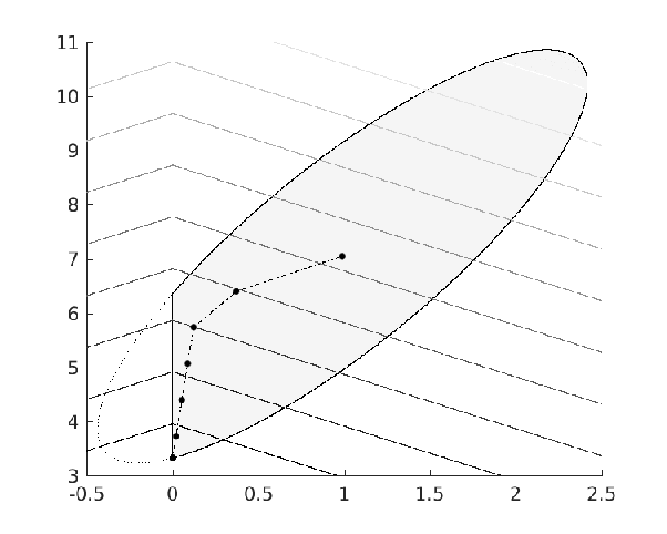
also suggested in [16]. Thus, in Algorithm 1, we have $\epsilon_{k}=0$ for all $k$ . In our tests, we set $x_{0}=\bar{x}$ and, for all $k$ , $\theta_{k}=0.25$ , $\lambda_{k}=0.025$ , $\gamma_{k}=0.025$ , and defined $\beta_{k}:=2(1-2\lambda_{k})/(1+2\gamma_{k})-10^{-6}$ satisfying (12). Figure 1 shows the behavior of SInexPD Algorithm on a two-dimensional instance of Problem (35). The hatched region represents set $C$ and only the iterates for which the target level was updated are plotted. As can be seen, the algorithm successfully found the solution for $\ell=6$ iterations. We point out that the algorithm performed a total of $\ell=14$ ( $k=189$ ) iterations until it met the stopping criterion. The highlight of the figure is that, before finding the solution, the iterates belong to the interior of set $C$ . This is mostly due to the fact that SInexPD Algorithm performs inexact projections.

Refer to caption — Figure 1: Behavior of SInexPD Algorithm on a two-dimensional instance of Problem (35).

Finally, we considered six instances of Problem (35) varying the dimension $n$ . Without attempting to go into details, we mention that the problems were randomly generated such that $\lambda_{n}\in(10^{-2},10^{-6})$ , $\lambda_{i}\in(10,10^{3})$ for $i=1,\ldots,n-1$ , vector $u\in\mathbb{R}^{n}_{++}$ in (36) is such that $\|u\|\in(0.8/\sqrt{\lambda_{n}},1/\sqrt{\lambda_{n}})$ , and $\xi=1\sqrt{\lambda_{n}}$ . These imply that, with respect to the ellipsoid that makes up set $C$ , the axis corresponding to the eigenvector $v_{n}$ is much larger than the others ones. Moreover, the vectors of $C$ that have only one non-null component are far from the center $\bar{x}$ . These characteristics make problems more challenging for the algorithm. Table 1 shows the performance of SInexPD Algorithm. In the table, column “ $n$ ” informs the considered dimension, “ $k$ ” and “ $\ell$ ” are the number of iterations according to SInexPD Algorithm, “ $\|x_{k}^{rec}\|_{0}$ ” is the number of non-null elements at the final iterate, and “ $f_{k}^{rec}$ ” and “ $\delta_{\ell}$ ” are their corresponding values at the final iterate.

$n$	$k$	$\ell$	$\\|x_{k}^{rec}\\|_{0}$	$f_{k}^{rec}$	$\delta_{\ell}$
10	91	19	1	1.12D+01	6.18D-03
100	85	21	1	1.07D+01	9.77D-03
200	63	36	1	2.11D+01	1.38D-02
500	58	22	1	1.01D+01	1.09D-02
800	575	26	1	1.20D+01	6.91D-03
1000	669	24	1	1.15D+01	7.72D-03

Table 1: Performance of SInexPD Algorithm on six instances of Problem (35) varying the dimension.

As showed in Table 1, the algorithm found vectors with only one non-null component in all instances, showing its ability to recover sparsity in this class of problems.

Remembering that the table data corresponds to the values when the stop criterion was met, we reported that the final iterates were found with $\ell=10,16,27,12,15$ and $12$ iterations, respectively. We point out that, due to the inexact projections and mimicking the behavior of SInexPD Algorithm in the two-dimensional case, in each instance the iterates remained in the interior of $C$ before the corresponding solution was found.

6 Conclusions

It is well known that the application of the subgradient method is only suitable for certain specific classes of non-differentiable convex optimization problems. However, this method is basic in the sense that it is the first step towards designing more efficient methods for solving that problems. Indeed, it is intrinsically related to cutting-plane and bundle methods; see [18]. These considerations lead us to conclude that the knowledge of new properties of the subgradient method has great theoretical value. In particular, our inexact version of the projected subgradient method will be useful in this theoretical context. Finally, one issue we believe deserves attention is the construction of inexact projected versions of cutting-plane and bundle methods.

References

[1] Y. I. Alber, A. N. Iusem, and M. V. Solodov. On the projected subgradient method for nonsmooth convex optimization in a Hilbert space. Math. Programming, 81(1, Ser. A):23–35, 1998.
[2] A. Beck and M. Teboulle. A conditional gradient method with linear rate of convergence for solving convex linear systems. Math. Methods Oper. Res., 59(2):235–247, 2004.
[3] J. Y. Bello Cruz. A subgradient method for vector optimization problems. SIAM J. Optim., 23(4):2169–2182, 2013.
[4] D. P. Bertsekas. Nonlinear programming. Athena Scientific Optimization and Computation Series. Athena Scientific, Belmont, MA, second edition, 1999.
[5] D. P. Bertsekas, A. Nedic, and A. E. Ozdaglar. Convex Analysis and Optimization. Athena Scientific Optimization and Computation Series. Athena Scientific, Belmont, MA, 2003.
[6] E. G. Birgin and J. M. Martínez. Practical augmented Lagrangian methods for constrained optimization. SIAM, 2014.
[7] U. Brannlund. On relaxation methods for nonsmooth convex optimization. ProQuest LLC, Ann Arbor, MI, 1993. Thesis (Takn.dr)–Kungliga Tekniska Hogskolan (Sweden).
[8] R. Burachik, L. M. G. Drummond, A. N. Iusem, and B. F. Svaiter. Full convergence of the steepest descent method with inexact line searches. Optimization, 32(2):137–146, 1995.
[9] R. Correa and C. Lemaréchal. Convergence of some algorithms for convex minimization. Math. Programming, 62(2, Ser. B):261–275, 1993.
[10] F. R. de Oliveira, O. P. Ferreira, and G. N. Silva. Newton’s method with feasible inexact projections for solving constrained generalized equations. Comput. Optim. Appl., 72(1):159–177, 2019.
[11] R. Díaz Millán, O. P. Ferreira, and L. F. Prudente. Alternating conditional gradient method for convex feasibility problems. arXiv e-prints, page arXiv:1912.04247, Dec 2019, 1912.04247.
[12] Y. M. Ermol’ev. Methods of solution of nonlinear extremal problems. Cybernetics, 2(4):1–14, 1966.
[13] M. Frank and P. Wolfe. An algorithm for quadratic programming. Naval Res. Logist. Quart., 3:95–110, 1956.
[14] M. Fukushima, Z.-Q. Luo, and P. Tseng. Smoothing functions for second-order-cone complementarity problems. SIAM J. Optim., 12(2):436–460, 2001/02.
[15] D. Garber and E. Hazan. Faster rates for the frank-wolfe method over strongly-convex sets. Proceedings of the 32Nd International Conference on International Conference on Machine Learning - Volume 37, pages 541–549, 2015.
[16] J.-L. Goffin and K. C. Kiwiel. Convergence of a simple subgradient level method. Math. Program., 85(1, Ser. A):207–211, 1999.
[17] N. I. M. Gould and P. L. Toint. Numerical methods for large-scale non-convex quadratic programming. In Trends in industrial and applied mathematics (Amritsar, 2001), volume 72 of Appl. Optim., pages 149–179. Kluwer Acad. Publ., Dordrecht, 2002.
[18] J.-B. Hiriart-Urruty and C. Lemaréchal. Convex analysis and minimization algorithms. II, volume 306 of Grundlehren der Mathematischen Wissenschaften [Fundamental Principles of Mathematical Sciences]. Springer-Verlag, Berlin, 1993. Advanced theory and bundle methods.
[19] M. Jaggi. Revisiting frank-wolfe: Projection-free sparse convex optimization. Proceedings of the 30th International Conference on Machine Learning, 28(1):427–435, 2013.
[20] K. C. Kiwiel. Methods of descent for nondifferentiable optimization, volume 1133 of Lecture Notes in Mathematics. Springer-Verlag, Berlin, 1985.
[21] I. V. Konnov. Simplified versions of the conditional gradient method. Optimization, 67(12):2275–2290, 2018.
[22] G. Lan and Y. Zhou. Conditional gradient sliding for convex optimization. SIAM J. Optim., 26(2):1379–1409, 2016.
[23] P.-E. Maingé. Strong convergence of projected subgradient methods for nonsmooth and nonstrictly convex minimization. Set-Valued Anal., 16(7-8):899–912, 2008.
[24] A. Nedić and D. Bertsekas. Convergence rate of incremental subgradient algorithms. In Stochastic optimization: algorithms and applications (Gainesville, FL, 2000), volume 54 of Appl. Optim., pages 223–264. Kluwer Acad. Publ., Dordrecht, 2001.
[25] A. Nedić and D. P. Bertsekas. Incremental subgradient methods for nondifferentiable optimization. SIAM J. Optim., 12(1):109–138, 2001.
[26] A. Nedić and D. P. Bertsekas. The effect of deterministic noise in subgradient methods. Math. Program., 125(1, Ser. A):75–99, 2010.
[27] Y. Nesterov. Introductory lectures on convex optimization, volume 87 of Applied Optimization. Kluwer Academic Publishers, Boston, MA, 2004. A basic course.
[28] Y. Nesterov. Subgradient methods for huge-scale optimization problems. Math. Program., 146(1-2, Ser. A):275–297, 2014.
[29] J. Nocedal and S. J. Wright. Numerical optimization. Springer Series in Operations Research and Financial Engineering. Springer, New York, second edition, 2006.
[30] B. T. Polyak. Minimization of nonsmooth functionals. Ž. Vyčisl. Mat. i Mat. Fiz., 9:509–521, 1969.
[31] B. T. Polyak. Introduction to optimization. Translations Series in Mathematics and Engineering. Optimization Software, Inc., Publications Division, New York, 1987. Translated from the Russian, With a foreword by Dimitri P. Bertsekas.
[32] S. N. Ravi, M. D. Collins, and V. Singh. A deterministic nonsmooth frank wolfe algorithm with coreset guarantees. INFORMS Journal on Optimization, 1(2):120–142, 2019, https://doi.org/10.1287/ijoo.2019.0014.
[33] N. Z. Shor. Minimization methods for nondifferentiable functions, volume 3 of Springer Series in Computational Mathematics. Springer-Verlag, Berlin, 1985. Translated from the Russian by K. C. Kiwiel and A. Ruszczyński.
[34] R. J. Vanderbei. Linear programming: foundations and extensions, volume 4 of International Series in Operations Research & Management Science. Kluwer Academic Publishers, Boston, MA, 1996.
[35] S. Villa, S. Salzo, L. Baldassarre, and A. Verri. Accelerated and inexact forward-backward algorithms. SIAM J. Optim., 23(3):1607–1633, 2013.
[36] X. M. Wang. Subgradient algorithms on Riemannian manifolds of lower bounded curvatures. Optimization, 67(1):179–194, 2018.

	$\displaystyle\\|w-x\\|^{2}$	$\displaystyle\leq\\|v-x\\|^{2}-(1-2\theta)\\|v-w\\|^{2}+2\gamma\\|v-u\\|^{2}+2\lambda\\|w-u\\|^{2}$
		$\displaystyle\leq\\|v-x\\|^{2}+2\gamma\\|v-u\\|^{2}+2\lambda\\|w-u\\|^{2}.$		(6)

	$\displaystyle\\|w-u\\|^{2}$	$\displaystyle=\\|v-u\\|^{2}+\\|w-v\\|^{2}+2\langle v-w,u-v\rangle$
		$\displaystyle=\\|v-u\\|^{2}+\\|w-v\\|^{2}+2\langle v-w,u-w\rangle-2\\|w-v\\|^{2}$
		$\displaystyle=\\|v-u\\|^{2}-\\|w-v\\|^{2}+2\langle v-w,u-w\rangle.$