跳到论文正文
W Papers独立论文阅读器 arXiv:2006.08737 论文正文 计算阅读时间 · 0%
引用这篇论文根据当前论文元数据生成,正式投稿前建议核对。


License: arXiv.org perpetual non-exclusive license
arXiv:2006.08737v1 [cs.LG] 15 Jun 2020

Distributed Newton Can Communicate Less and Resist Byzantine Workers

Avishek Ghosh Affiliation: Department of EECS, UC Berkeley Affiliation: Berkeley, CA 94720 Email: avishek_ghosh@berkeley.edu    Raj Kumar Maity Affiliation: College of Information and Computer Sciences Affiliation: UMass Amherst, MA-01002 Email: rajkmaity@cs.umass.edu    Arya Mazumdar Affiliation: College of Information and Computer Sciences Affiliation: UMass Amherst, MA-01002 Email: arya@cs.umass.edu
Abstract

We develop a distributed second order optimization algorithm that is communication-efficient as well as robust against Byzantine failures of the worker machines. We propose COMRADE (COMunication-efficient and Robust Approximate Distributed nEwton), an iterative second order algorithm, where the worker machines communicate only once per iteration with the center machine. This is in sharp contrast with the state-of-the-art distributed second order algorithms like GIANT [34] and DINGO[7], where the worker machines send (functions of) local gradient and Hessian sequentially; thus ending up communicating twice with the center machine per iteration. Moreover, we show that the worker machines can further compress the local information before sending it to the center. In addition, we employ a simple norm based thresholding rule to filter-out the Byzantine worker machines. We establish the linear-quadratic rate of convergence of COMRADE and establish that the communication savings and Byzantine resilience result in only a small statistical error rate for arbitrary convex loss functions. To the best of our knowledge, this is the first work that addresses the issue of Byzantine resilience in second order distributed optimization. Furthermore, we validate our theoretical results with extensive experiments on synthetic and benchmark LIBSVM [5] data-sets and demonstrate convergence guarantees.

1 Introduction

In modern data-intensive applications like image recognition, conversational AI and recommendation systems, the size of training datasets has grown in such proportions that distributed computing have become an integral part of machine learning. To this end, a fairly common distributed learning framework, namely data parallelism, distributes the (huge) data-sets over multiple worker machines to exploit the power of parallel computing. In many applications, such as Federated Learning [20], data is stored in users’ personal devices and judicious exploitation of the on-device machine intelligence can speed up computation. Usually, in a distributed learning framework, computation (such as processing, training) happens in the worker machines and the local results are communicated to a center machine (ex., a parameter server). The center machine updates the model parameters by properly aggregating the local results.

Such distributed frameworks face the following two fundamental challenges: First, the parallelism gains are often bottle-necked by the heavy communication overheads between worker and the center machines. This issue is further exacerbated where large clusters of worker machines are used for modern deep learning applications using models with millions of parameters (NLP models, such as BERT [10], may have well over 100 million parameters). Furthermore, in Federated Learning, this uplink cost is tied to the user’s upload bandwidth. Second, the worker machines might be susceptible to errors owing to data crashes, software or hardware bugs, stalled computation or even malicious and co-ordinated attacks. This inherent unpredictable (and potentially adversarial) nature of worker machines is typically modeled as Byzantine failures. As shown in [21], Byzantine behavior a single worker machine can be fatal to the learning algorithm.

Both these challenges, communication efficiency and Byzantine-robustness, have been addressed in a significant number of recent works, albeit mostly separately. For communication efficiency, several recent works [32, 30, 2, 14, 1, 35, 19] use quantization or sparsification schemes to compress the message sent by the worker machines to the center machine. An alternative, and perhaps more natural way to reduce the communication cost (via reducing the number of iterations) is to use second order optimization algorithms; which are known to converge much faster than their first order counterparts. Indeed, a handful of algorithms has been developed using this philosophy, such as DANE [27], DISCO [38], GIANT [34] , DINGO [7], Newton-MR [26], INEXACT DANE and AIDE [25]. In a recent work [17], second order optimization and compression schemes are used simultaneously for communication efficiency. On the other hand, the problem of developing Byzantine-robust distributed algorithms has also been considered recently (see [29, 13, 6, 36, 37, 15, 4] ). However, all of these papers analyze different variations of the gradient descent, the standard first order optimization algorithm.

In this work, we propose COMRADE, a distributed approximate Newton-type algorithm that communicates less and is resilient to Byzantine workers. Specifically, we consider a distributed setup with mm worker machines and one center machine. The goal is to minimize a regularized convex loss f:ℝd→ℝf:\mathbb{R}^{d}\to\mathbb{R}, which is additive over the available data points. Furthermore, we assume that α\alpha fraction of the worker machines are Byzantine, where α∈[0,1/2)\alpha\in[0,1/2). We assume that Byzantine workers can send any arbitrary values to the center machine. In addition, they may completely know the learning algorithm and are allowed to collude with each other. To the best of our knowledge, this is the first paper that addresses the problem of Byzantine resilience in second order optimization.

In our proposed algorithm, the worker machines communicate only once per iteration with the center machine. This is in sharp contrast with the state-of-the-art distributed second order algorithms (like GIANT [34], DINGO [7], Determinantal Averaging [9]), which sequentially estimates functions of local gradients and Hessians and communicate them with the center machine. In this way, they end up communicating twice per iteration with the center machine. We show that this sequential estimation is redundant. Instead, in COMRADE, the worker machines only send a dd dimensional vector, the product of the inverse of local Hessian and the local gradient. Via sketching arguments, we show that the empirical mean of the product of local Hessian inverse and local gradient is close to the global Hessian inverse and gradient product, and thus just sending the above-mentioned product is sufficient to ensure convergence. Hence, in this way, we save 𝒪⁡(d)\mathcal{O}(d) bits of communication per iteration. Furthermore, in Section 5, we argue that, in order to cut down further communication, the worker machines can even compress the local Hessian inverse and gradient product. Specifically, we use a (generic) ρ\rho-approximate compressor ([19]) for this, that encompasses sign-based compressors like QSGD [1] and topk sparsification [28].

For Byzantine resilience, COMRADE employs a simple thresholding policy on the norms of the local Hessian inverse and local gradient product. Note that norm-based thresholding is computationally much simpler in comparison to existing co-ordinate wise median or trimmed mean ([36]) algorithms. Since the norm of the Hessian-inverse and gradient product determines the amount of movement for Newton-type algorithms, this norm corresponds to a natural metric for identifying and filtering out Byzantine workers.

Our Contributions:

We propose a communication efficient Newton-type algorithm that is robust to Byzantine worker machines. Our proposed algorithm, COMRADE takes as input the local Hessian inverse and gradient product (or a compressed version of it) from the worker machines, and performs a simple thresholding operation on the norm of the said vector to discard β>α\beta>\alpha fraction of workers having largest norm values. We prove the linear-quadratic rate of convergence of our proposed algorithm for strongly convex loss functions. In particular, suppose there are mm worker machines, each containing ss data points; and let 𝚫t=𝐰t−𝐰∗\mathbf{\Delta}_{t}=\mathbf{w}_{t}-\mathbf{w}^{*}, where 𝐰t\mathbf{w}_{t} is the tt-th iterate of COMRADE, and 𝐰∗\mathbf{w}^{*} is the optimal model we want to estimate. In Theorem 2, we show that

‖𝚫t+1‖≤max⁡{Ψt(1)​‖𝚫t‖,Ψt(2)​‖𝚫t‖2}+(Ψt(3)+α)​1s,\displaystyle\|\mathbf{\Delta}_{t+1}\|\leq\max\{\Psi^{(1)}_{t}\|\mathbf{\Delta}_{t}\|,\Psi^{(2)}_{t}\|\mathbf{\Delta}_{t}\|^{2}\}+(\Psi^{(3)}_{t}+\alpha)\sqrt{\frac{1}{s}},

where {Ψt(i)}i=13\{\Psi^{(i)}_{t}\}_{i=1}^{3} are quantities dependent on several problem parameters. Notice that the above implies a quadratic rate of convergence when ‖𝚫t‖≥Ψt(1)/Ψt(2)\|\mathbf{\Delta}_{t}\|\geq\Psi^{(1)}_{t}/\Psi^{(2)}_{t}. Subsequently, when ‖𝚫t‖\|\mathbf{\Delta}_{t}\| becomes sufficiently small, the above condition is violated and the convergence slows down to a linear rate. The error-floor, which is 𝒪⁡(1/s)\mathcal{O}(1/\sqrt{s}) comes from the Byzantine resilience subroutine in conjunction with the simultaneous estimation of Hessian and gradient. Furthermore, in Section 5, we consider worker machines compressing the local Hessian inverse and gradient product via a ρ\rho-approximate compressor [19], and show that the (order-wise) rate of convergence remain unchanged, and the compression factor, ρ\rho affects the constants only.

We experimentally validate our proposed algorithm, COMRADE, with several benchmark data-sets. We consider several types of Byzantine attacks and observe that COMRADE is robust against Byzantine worker machines, yielding better classification accuracy compared to the existing state-of-the-art second order algorithms.

A major technical challenge of this paper is to approximate local gradient and Hessian simultaneously in the presence of Byzantine workers. We use sketching, similar to [34], along with the norm based Byzantine resilience technique. Using incoherence (defined shortly) of the local Hessian along with concentration results originating from uniform sampling, we obtain the simultaneous gradient and Hessian approximation. Furthermore, ensuring at least one non-Byzantine machine gets trimmed at every iteration of COMRADE, we control the influence of Byzantine workers.

Related Work:

Second order Optimization: Second order optimization has received a lot of attention in the recent years in the distributed setting owing to its attractive convergence speed. The fundamentals of second order optimization is laid out in [27], and an extension with better convergence rates is presented in [25]. Recently, in GIANT [34] algorithm, each worker machine computes an approximate Newton direction in each iteration and the center machine averages them to obtain a globally improved approximate Newton direction. Furthermore, DINGO [7] generalizes second order optimization beyond convex functions by extending the Newton-MR [26] algorithm in a distributed setting. Very recently, [9] proposes Determinantal averaging to correct the inversion bias of the second order optimization. A slightly different line of work ([33], [18], [24]) uses Hessian sketching to solve a large-scale distributed learning problems.

Byzantine Robust Optimization: In the seminal work of [13], a generic framework of one shot median based robust learning has been proposed and analyzed in the distributed setting. The issue of Byzantine failure is tackled by grouping the servers in batches and computing the median of batched servers in [6] (the median of means algorithm). Later in [36, 37], co-ordinate wise median, trimmed mean and iterative filtering based algorithm have been proposed and optimal statistical error rate is obtained. Also, [23, 8] consider adversaries may steer convergence to bad local minimizers for non-convex optimization problems. Byzantine resilience with gradient quantization has been addressed in the recent works of [3, 16].

Organization:

In Section 3, we first analyze COMRADE with one round of communication per iteration. We assume α=0\alpha=0, and focus on the communication efficiency aspect only. Subsequently, in Section 4, we make α≠0\alpha\neq 0, thereby addressing communication efficiency and Byzantine resilience simultaneously. Further, in Section 5 we augment a compression scheme along with the setting of Section 4. Finally, in Section 6, we validate our theoretical findings with experiments. Proofs of all theoretical results can be found in the supplementary material.

Notation:

For a positive integer rr, [r][r] denotes the set {1,2,…,r}\{1,2,\ldots,r\}. For a vector vv, we use ‖v‖\|v\| to denote the ℓ2\ell_{2} norm unless otherwise specified. For a matrix XX, we denote ‖X‖2\|X\|_{2} denotes the operator norm, σm​a​x​(X)\sigma_{max}(X) and σm​i​n​(X)\sigma_{min}(X) denote the maximum and minimum singular value. Throughout the paper, we use C,C1,c,c1C,C_{1},c,c_{1} to denote positive universal constants, whose value changes with instances.

2 Problem Formulation

We begin with the standard statistical learning framework for empirical risk minimization, where the objective is to minimize the following loss function:

f⁡(𝐰)=1n​∑j=1nℓj​(𝐰T​𝐱j)+λ2​‖𝐰‖2,\displaystyle f(\mathbf{w})=\frac{1}{n}\sum_{j=1}^{n}\ell_{j}(\mathbf{w}^{T}\mathbf{x}_{j})+\frac{\lambda}{2}\|\mathbf{w}\|^{2}, (1)

where, the loss functions ℓj:ℝ→ℝ\ell_{j}:\mathbb{R}\rightarrow\mathbb{R}, j∈[n]j\in[n] are convex, twice differentiable and smooth. Moreover, 𝐱1,𝐱2,…,𝐱n∈ℝd\mathbf{x}_{1},\mathbf{x}_{2},\ldots,\mathbf{x}_{n}\,\in\mathbb{R}^{d} denote the input feature vectors and y1,y2,…,yn∈y_{1},y_{2},\ldots,y_{n}\in\real denote the corresponding responses. Furthermore, we assume that the function ff is strongly convex, implying the existence of a unique minimizer of (1). We denote this minimizer by 𝐰∗\mathbf{w}^{*}. Note that the response {yj}j=1n\{y_{j}\}_{j=1}^{n} is captured by the corresponding loss function {ℓj}j=1n\{\ell_{j}\}_{j=1}^{n}. Some examples of ℓj\ell_{j} are

logistic loss: ℓj(zj)=log(1−exp(−zjyj)),squared loss: ℓj(zj)=12(zj−yj)2\displaystyle\text{logistic loss: }\,\,\ell_{j}(z_{j})=\log(1-\exp(-z_{j}y_{j})),\quad\text{squared loss: }\,\,\ell_{j}(z_{j})=\frac{1}{2}(z_{j}-y_{j})^{2}

We consider the framework of distributed optimization with mm worker machines, where the feature vectors and the loss functions (𝐱1,ℓ1),…,(𝐱n,ℓn)(\mathbf{x}_{1},\ell_{1}),\ldots,(\mathbf{x}_{n},\ell_{n}) are partitioned homogeneously among them. Furthermore, we assume that α\alpha fraction of the worker machines are Byzantine for some α<12\alpha<\frac{1}{2}. The Byzantine machines, by nature, may send any arbitrary values to the center machine. Moreover, they can even collude with each other and plan malicious attacks with complete information of the learning algorithm.

3 COMRADE Can Communicate Less

We first present the Newton-type learning algorithm, namely COMRADE without any Byzantine workers, i.e., α=0\alpha=0. It is formally given in Algorithm 1 (with β=0\beta=0). In each iteration of our algorithm, every worker machine computes the local Hessian and local gradient and sends the local second order update (which is the product of the inverse of the local Hessian and local gradient) to the center machine. The center machine aggregates the updates from the worker machines by averaging them and updates the model parameter 𝐰\mathbf{w}. Later the center machine broadcast the parameter 𝐰\mathbf{w} to all the worker machines.

In any iteration tt, a standard Newton algorithm requires the computation of exact Hessian (𝐇t)(\mathbf{H}_{t}) and gradient (𝐠t)(\mathbf{g}_{t}) of the loss function which can be written as

𝐠t=1n∑i=1nℓj′(𝐰t⊤𝐱i)𝐱i+λ𝐰t,𝐇t=1n∑i=1nℓj′′(𝐰t⊤𝐱i)𝐱i𝐱i⊤+λ𝐈.\displaystyle\mathbf{g}_{t}=\frac{1}{n}\sum_{i=1}^{n}\ell_{j}^{\prime}(\mathbf{w}_{t}^{\top}\mathbf{x}_{i})\mathbf{x}_{i}+\lambda\mathbf{w}_{t},\,\,\mathbf{H}_{t}=\frac{1}{n}\sum_{i=1}^{n}\ell_{j}^{{}^{\prime\prime}}(\mathbf{w}_{t}^{\top}\mathbf{x}_{i})\mathbf{x}_{i}\mathbf{x}_{i}^{\top}+\lambda\mathbf{I}.\vskip-5.69054pt (2)

In a distributed set up, the exact Hessian (𝐇t)(\mathbf{H}_{t}) and gradient (𝐠t)(\mathbf{g}_{t}) can be computed in parallel in the following manner. In each iteration, the center machine ‘broadcasts’ the model parameter 𝐰t\mathbf{w}_{t} to the worker machines and each worker machine computes its own local gradient and Hessian. Then the center machine can compute the exact gradient and exact Hessian by averaging the the local gradient vectors and local Hessian matrices. But for each worker machine the per iteration communication complexity is 𝒪⁡(d)\mathcal{O}(d) for the gradient computation and 𝒪⁡(d2CLOSE\mathcal{O}(d^{2}) for the Hessian computation. Using Algorithm 1, we reduce the communication cost to only 𝒪⁡(d)\mathcal{O}(d) per iteration, which is the same as the first order methods.

Each worker machine possess ss samples drawn uniformly from {(𝐱1,ℓ1),(𝐱2,ℓ2),…,(𝐱n,ℓn)}\{(\mathbf{x}_{1},\ell_{1}),(\mathbf{x}_{2},\ell_{2}),\ldots,(\mathbf{x}_{n},\ell_{n})\}. By SiS_{i}, we denote the indices of the samples held by worker machine ii. At any iteration tt, the worker machine computes the local Hessian 𝐇i,t\mathbf{H}_{i,t} and local gradient 𝐠i,t\mathbf{g}_{i,t} as

𝐠i,t=1s∑i∈Siℓj′(𝐰t⊤𝐱i)𝐱i+λ𝐰t,𝐇i,t=1s∑i∈Siℓj′′(𝐰t⊤𝐱i)𝐱i𝐱i⊤+λ𝐈.\displaystyle\mathbf{g}_{i,t}=\frac{1}{s}\sum_{i\in S_{i}}\ell_{j}^{\prime}(\mathbf{w}_{t}^{\top}\mathbf{x}_{i})\mathbf{x}_{i}+\lambda\mathbf{w}_{t},\quad\mathbf{H}_{i,t}=\frac{1}{s}\sum_{i\in S_{i}}\ell_{j}^{{}^{\prime\prime}}(\mathbf{w}_{t}^{\top}\mathbf{x}_{i})\mathbf{x}_{i}\mathbf{x}_{i}^{\top}+\lambda\mathbf{I}. (3)

It is evident from the uniform sampling that 𝔼⁡[𝐠i,t]=𝐠t\mathbb{E}[\mathbf{g}_{i,t}]=\mathbf{g}_{t} and 𝔼⁡[𝐇i,t]=𝐇t\mathbb{E}[\mathbf{H}_{i,t}]=\mathbf{H}_{t}. The update direction from the worker machine is defined as 𝐩^i,t=(𝐇i,t)−1​𝐠i,t\hat{\mathbf{p}}_{i,t}=(\mathbf{H}_{i,t})^{-1}\mathbf{g}_{i,t}. Each worker machine requires O⁡(s​d2)O(sd^{2}) operations to compute the Hessian matrix 𝐇i,t\mathbf{H}_{i,t} and O⁡(d3)O(d^{3}) operations to invert the matrix. In practice, the computational cost can be reduced by employing conjugate gradient method. The center machine computes the parameter update direction 𝐩^t=1m​∑i=1m𝐩^i,t\hat{\mathbf{p}}_{t}=\frac{1}{m}\sum_{i=1}^{m}\hat{\mathbf{p}}_{i,t}.

We show that given large enough sample in each worker machine (ss is large) and with incoherent data points (the information is spread out and not concentrated to a small number of sample data points), the local Hessian 𝐇i,t\mathbf{H}_{i,t} is close to the global Hessian 𝐇t\mathbf{H}_{t} in spectral norm, and the local gradient 𝐠i,t\mathbf{g}_{i,t} is close to the global gradient 𝐠t\mathbf{g}_{t}. Subsequently, we prove that the empirical average of the local updates acts as a good proxy for the global Newton update and achieves good convergence guarantee.

Algorithm 1 COMmunication-efficient and Robust Approximate Distributed nEwton (COMRADE)
1:  Input: Step size γ\gamma, parameter β≥0\beta\geq 0
2:  Initialize: Initial iterate w0∈ℝdw_{0}\in\mathbb{R}^{d}
3:  for t=0,1,…,T−1t=0,1,\ldots,T-1 do
4:   Central machine: broadcasts wtw_{t} for i∈[m]i\in[m] do in parallel
5:   ii-th worker machine:
  • •

    Non-Byzantine: Computes local gradient 𝐠i,t\mathbf{g}_{i,t} and local Hessian 𝐇i,t\mathbf{H}_{i,t}; sends 𝐩^i,t=(𝐇i,t)−1​𝐠i,t\hat{\mathbf{p}}_{i,t}=(\mathbf{H}_{i,t})^{-1}\mathbf{g}_{i,t} to the central machine,

  • •

    Byzantine: Generates ⋆\star (arbitrary), and sends it to the center machine

end for
6:   Center Machine:
  • •

    Sort the worker machines in a non decreasing order according to norm of updates {𝐩^i,t}i=1m\{\hat{\mathbf{p}}_{i,t}\}_{i=1}^{m} from the local machines

  • •

    Return the indices of the first 1−β1-\beta fraction of machines as 𝒰t\mathcal{U}_{t},

  • •

    Approximate Newton Update direction : 𝐩^t=1|𝒰t|​∑i∈𝒰t𝐩^i,t\hat{\mathbf{p}}_{t}=\frac{1}{|\mathcal{U}_{t}|}\sum_{i\in\mathcal{U}_{t}}\hat{\mathbf{p}}_{i,t}

  • •

    Update model parameter: wt+1=wt−γ​𝐩^tw_{t+1}=w_{t}-\gamma\hat{\mathbf{p}}_{t}.

7:  end for

3.1 Theoretical Guarantee

We define the matrix 𝐀t⊤=[𝐚1⊤,…,𝐚n⊤]∈ℝd×n\mathbf{A}_{t}^{\top}=[\mathbf{a}_{1}^{\top},\ldots,\mathbf{a}_{n}^{\top}]\in\mathbb{R}^{d\times n} where 𝐚j=ℓj′′​(𝐰⊤​𝐱j)​𝐱j\mathbf{a}_{j}=\sqrt{\ell^{\prime\prime}_{j}(\mathbf{w}^{\top}\mathbf{x}_{j})}\,\mathbf{x}_{j}. So the exact Hessian in equation (2) is 𝐇t=1n​𝐀t⊤​𝐀t+λ​𝐈\mathbf{H}_{t}=\frac{1}{n}\mathbf{A}_{t}^{\top}\mathbf{A}_{t}+\lambda\mathbf{I}. Also we define 𝐁t=[𝐛1,…,𝐛n]∈ℝd×n\mathbf{B}_{t}=[\mathbf{b}_{1},\ldots,\mathbf{b}_{n}]\in\mathbb{R}^{d\times n} where 𝐛i=ℓi′​(𝐰T​𝐱i)​𝐱i\mathbf{b}_{i}=\ell^{\prime}_{i}(\mathbf{w}^{T}\mathbf{x}_{i})\mathbf{x}_{i}. So the exact gradient in equation (2) is 𝐠t=1n​𝐁t​𝟏+λ​𝐰t\mathbf{g}_{t}=\frac{1}{n}\mathbf{B}_{t}\mathbf{1}+\lambda\mathbf{w}_{t}

Definition 1 (Coherence of a Matrix).

Let 𝐀∈ℝn×d\mathbf{A}\in\mathbb{R}^{n\times d} be any matrix with 𝐔∈ℝn×d\mathbf{U}\in\mathbb{R}^{n\times d} being its orthonormal basis (the left singular vectors). The row coherence of the matrix 𝐀\mathbf{A} is defined as μ⁡(𝐀)=nd​maxi​‖𝐮i‖2∈[1,nd]\mu(\mathbf{A})=\frac{n}{d}\max_{i}\left\|\mathbf{u}_{i}\right\|^{2}\in\left[1,\frac{n}{d}\right], where 𝐮i\mathbf{u}_{i} is the iith row of 𝐔\mathbf{U}.

Remark 1.

If the coherence of 𝐀t\mathbf{A}_{t} is small, it can be shown that the Hessian matrix can be approximated well via selecting a subset of rows. Note that this is a fairly common to use coherence condition as an approximation tool (see [11, 12, 22])

In the following, we assume that the Hessian matrix is LL-Lipschitz (see definition below), which is a standard assumption for the analysis of the second order method for general smooth loss function (as seen in [34],[9]).

Assumption 1.

The Hessian matrix of the loss function ff is LL-Lipschitz continuous i.e. ‖∇2f​(w)−∇2f​(w′)‖2≤L⁡‖w−w′‖\left\|\nabla^{2}f(w)-\nabla^{2}f(w^{\prime})\right\|_{2}\leq L\left\|w-w^{\prime}\right\|.

In the following theorem, we provide the convergence rate of COMRADE (with α=β=0\alpha=\beta=0) in the terms of 𝚫t=𝐰t−𝐰∗\mathbf{\Delta}_{t}=\mathbf{w}_{t}-\mathbf{w}^{*}. Also, we define κt=σm​a​x​(𝐇t)/σm​i​n​(𝐇t)\kappa_{t}=\sigma_{max}(\mathbf{H}_{t})/\sigma_{min}(\mathbf{H}_{t}) as the condition number of 𝐇t\mathbf{H}_{t}, and hence κt≥1\kappa_{t}\geq 1.

Theorem 1.

Let μ∈[1,nd]\mu\in\left[1,\frac{n}{d}\right] be the coherence of 𝐀t\mathbf{A}_{t} . Suppose γ=1\gamma=1 and s≥3​μ​dη2​log⁡m​dδs\geq\frac{3\mu d}{\eta^{2}}\log\frac{md}{\delta} for some η,δ∈(0,1)\eta,\delta\in(0,1). Under Assumption  1 , with probability exceeding 1−δ1-\delta, we obtain

‖𝚫t+1‖≤max⁡{κt​(ζ21−ζ2)​‖𝚫t‖,Lσm​i​n​(𝐇t)​‖𝚫t‖2}+2​ϵσm​i​n​(𝐇t),\displaystyle\|\mathbf{\Delta}_{t+1}\|\leq\max\{\sqrt{\kappa_{t}(\frac{\zeta^{2}}{1-\zeta^{2}})}\|\mathbf{\Delta}_{t}\|,\frac{L}{\sigma_{min}(\mathbf{H}_{t})}\|\mathbf{\Delta}_{t}\|^{2}\}+\frac{2\epsilon}{\sqrt{\sigma_{min}(\mathbf{H}_{t})}},

where ζ=ν⁡(ηm+η21−η)\zeta=\nu(\frac{\eta}{\sqrt{m}}+\frac{\eta^{2}}{1-\eta}), ν=σm​a​x​(𝐀⊤​𝐀)σm​a​x​(𝐀⊤​𝐀)+n​λ≤1\nu=\frac{\sigma_{max}(\mathbf{A}^{\top}\mathbf{A})}{\sigma_{max}(\mathbf{A}^{\top}\mathbf{A})+n\lambda}\leq 1, and

ϵ=11−η​1σm​i​n​(𝐇t)​(1+2​ln⁡(mδ))​1s​maxi​‖𝐛i‖.\displaystyle\epsilon=\frac{1}{1-\eta}\frac{1}{\sqrt{\sigma_{min}(\mathbf{H}_{t})}}(1+\sqrt{2\ln(\frac{m}{\delta})})\sqrt{\frac{1}{s}}\max_{i}\|\mathbf{b}_{i}\|. (4)
Remark 2.

It is well known that a distributed Newton method has linear-quadratic convergence rate. In Theorem 1 the quadratic term comes from the standard analysis of Newton method. The linear term (which is small) arises owing to Hessian approximation. It gets smaller with better Hessian approximation (smaller η\eta), and thus the above rate becomes quadratic one. The small error floor arises due to the gradient approximation in the worker machines, which is essential for the one round of communication per iteration. The error floor is ∝1s\propto\frac{1}{\sqrt{s}} where ss is the number of samples in each worker machine. So for a sufficiently large ss, the error floor becomes negligible.

Remark 3.

The sample size in each worker machine is dependent on the coherence of the matrix 𝐀t\mathbf{A}_{t} and the dimension dd of the problem. Theoretically, the analysis is feasible for the case of s≥ds\geq d (since we work with 𝐇i,t−1\mathbf{H}_{i,t}^{-1}). However, when s<ds<d, one can replace the inverse by a pseudo-inverse (modulo some changes in convergence rate).

4 COMRADE Can Resist Byzantine Workers

In this section, we analyze COMRADE with Byzantine workers. We assume that α(<1/2)\alpha(<1/2) fraction of worker machines are Byzantine. We define the set of Byzantine worker machines by ℬ\mathcal{B} and the set of the good (non-Byzantine) machines by ℳ\mathcal{M}. COMRADE employs a ‘norm based thresholding’ scheme on the local Hessian inverse and gradient product to tackle the Byzantine workers.

In the tt-th iteration, the center machine outputs a set 𝒰t\mathcal{U}_{t} with |𝒰t|=(1−β)​m\left|\mathcal{U}_{t}\right|=(1-\beta)m, consisting the indices of the worker machines with smallest norm. Hence, we ‘trim’ the worker machines that may try to diverge the learning algorithm. We denote the set of trimmed machines as 𝒯t\mathcal{T}_{t}. Moreover, we take β>α\beta>\alpha to ensure at least one good machine falls in 𝒯t\mathcal{T}_{t}. This condition helps us to control the Byzantine worker machines. Finally, the update is given by 𝐩^t=1|𝒰t|​∑i∈𝒰t𝐩^i,t\hat{\mathbf{p}}_{t}=\frac{1}{|\mathcal{U}_{t}|}\sum_{i\in\mathcal{U}_{t}}\hat{\mathbf{p}}_{i,t}. We define:

ϵb​y​z2=[3​(1−α1−β)2+4​κt​(α1−β)2]​ϵ2,\displaystyle\epsilon_{byz}^{2}=[3(\frac{1-\alpha}{1-\beta})^{2}+4\kappa_{t}(\frac{\alpha}{1-\beta})^{2}]\epsilon^{2}, (5)
ζb​y​z2=2​(1−α1−β)2​(ν1−η)2+ν2​(1−α1−β)2​(η(1−α)​m+η21−η)2+4​κt​(α1−β)2​[2+(ν1−η)2].\displaystyle\zeta^{2}_{byz}=2(\frac{1-\alpha}{1-\beta})^{2}(\frac{\nu}{1-\eta})^{2}+\nu^{2}(\frac{1-\alpha}{1-\beta})^{2}(\frac{\eta}{\sqrt{(1-\alpha)m}}+\frac{\eta^{2}}{1-\eta})^{2}+4\kappa_{t}(\frac{\alpha}{1-\beta})^{2}[2+(\frac{\nu}{1-\eta})^{2}]. (6)

ϵ\epsilon is defined in (4), ν=σm​a​x​(𝐀T​𝐀)σm​a​x​(𝐀T​𝐀)+n​λ\nu=\frac{\sigma_{max}(\mathbf{A}^{T}\mathbf{A})}{\sigma_{max}(\mathbf{A}^{T}\mathbf{A})+n\lambda} and κt\kappa_{t} is the condition number of the exact Hessian 𝐇t\mathbf{H}_{t}.

Theorem 2.

Let μ∈[1,nd]\mu\in\left[1,\frac{n}{d}\right] be the coherence of 𝐀t\mathbf{A}_{t} . Suppose γ=1\gamma=1 and s≥3​μ​dη2​log⁡m​dδs\geq\frac{3\mu d}{\eta^{2}}\log\frac{md}{\delta} for some η,δ∈(0,1)\eta,\delta\in(0,1). For 0≤α<β<1/20\leq\alpha<\beta<1/2 , under Assumption  1 , with probability exceeding 1−δ1-\delta, Algorithm 1 yields

‖𝚫t+1‖≤max⁡{κt​(ζb​y​z21−ζb​y​z2)​‖𝚫t‖,Lσm​i​n​(𝐇t)​‖𝚫t‖2}+2​ϵb​y​zσm​i​n​(𝐇t),\displaystyle\|\mathbf{\Delta}_{t+1}\|\leq\max\{\sqrt{\kappa_{t}(\frac{\zeta_{byz}^{2}}{1-\zeta_{byz}^{2}})}\|\mathbf{\Delta}_{t}\|,\frac{L}{\sigma_{min}(\mathbf{H}_{t})}\|\mathbf{\Delta}_{t}\|^{2}\}+\frac{2\epsilon_{byz}}{\sqrt{\sigma_{min}(\mathbf{H}_{t})}},

where ζb​y​z\zeta_{byz} and ϵb​y​z\epsilon_{byz} are defined in equations (5) and (6) respectively.

The remarks of Section 3 is also applicable here. On top of that, we have the following remarks:

Remark 4.

Compared to the convergence rate of Theorem 1, the rate here remains order-wise same even with Byzantine robustness. The coefficient of the quadratic term remains unchanged but the linear rate and the error floor suffers a little bit (by a small constant factor).

Remark 5.

Note that for Theorem 2 to hold, we require α∼1/κt\alpha\sim 1/\sqrt{\kappa_{t}} for all tt. In cases where κt\kappa_{t} is large, this can impose a stricter condition on α\alpha. However, we conjecture that this dependence can be improved via applying a more intricate (and perhaps computation heavy) Byzantine resilience algorithm. In this work, we kept the Byzantine resilience scheme simple at the expense of this condition on α\alpha.

5 COMRADE Can Communicate Even Less and Resist Byzantine Workers

In Section 3 we analyze COMRADE with an additional feature. We let the worker machines further reduce the communication cost by applying a generic class of ρ\rho-approximate compressor [19] on the parameter update of Algorithm 1. We first define the class of ρ\rho-approximate compressor:

Definition 2.

An operator 𝒬:ℝd→ℝd\mathcal{Q}:\mathbb{R}^{d}\rightarrow\mathbb{R}^{d} is defined as ρ\rho-approximate compressor on a set S⊂ℝdS\subset\mathbb{R}^{d} if, ∀x∈S\forall x\in S, ‖𝒬⁡(x)−x‖2≤(1−ρ)​‖x‖2\left\|\mathcal{Q}(x)-x\right\|^{2}\leq(1-\rho)\left\|x\right\|^{2}, where ρ∈[0,1]\rho\in[0,1] is the compression factor.

The above definition can be extended for any randomized operator 𝒬\mathcal{Q} satisfying 𝔼⁡(‖𝒬⁡(x)−x‖2)≤(1−ρ)​‖x‖2\mathbb{E}(\left\|\mathcal{Q}(x)-x\right\|^{2})\leq(1-\rho)\left\|x\right\|^{2}, for all ∀x∈S\forall x\in S. The expectation is taken over the randomization of the operator. Notice that ρ=1\rho=1 implies that 𝒬⁡(x)=x\mathcal{Q}(x)=x (no compression). Examples of ρ\rho-approximate compressor include QSGD [1], ℓ1\ell_{1}-QSGD [19], topk sparsification and randk [28].

Worker machine ii computes the product of local Hessian inverse inverse and local gradient and then apply ρ\rho-approximate compressor to obtain 𝒬⁡(𝐇i,t−1​𝐠i,t)\mathcal{Q}(\mathbf{H}_{i,t}^{-1}\mathbf{g}_{i,t}); and finally sends this compressed vector to the center. The Byzantine resilience subroutine remains the same–except, instead of sorting with respect to ‖𝐇i,t−1​𝐠i,t‖\|\mathbf{H}_{i,t}^{-1}\mathbf{g}_{i,t}\|, the center machine now sorts according to ‖𝒬⁡(𝐇i,t−1​𝐠i,t)‖\|\mathcal{Q}(\mathbf{H}_{i,t}^{-1}\mathbf{g}_{i,t})\|. The center machine aggregates the compressed updates by averaging 𝒬⁡(𝐩^)=1|𝒰t|​∑i∈𝒰t𝒬⁡(𝐩^i,t)\mathcal{Q}(\hat{\mathbf{p}})=\frac{1}{|\mathcal{U}_{t}|}\sum_{i\in\mathcal{U}_{t}}\mathcal{Q}(\hat{\mathbf{p}}_{i,t}), and take the next step as wt+1=wt−γ​𝒬​(𝐩^)w_{t+1}=w_{t}-\gamma\mathcal{Q}(\hat{\mathbf{p}}).

Recall the definition of ϵ\epsilon from (4). We also use the following notation : ζℳ2=ν⁡(η(1−α)​m+η21−η),ζ1=ν1−η\zeta^{2}_{\mathcal{M}}=\nu(\frac{\eta}{\sqrt{(1-\alpha)m}}+\frac{\eta^{2}}{1-\eta}),\zeta_{1}=\frac{\nu}{1-\eta} and ν=σm​a​x​(𝐀T​𝐀)σm​a​x​(𝐀T​𝐀)+n​λ\nu=\frac{\sigma_{max}(\mathbf{A}^{T}\mathbf{A})}{\sigma_{max}(\mathbf{A}^{T}\mathbf{A})+n\lambda}. Furthermore, we define the following:

ϵc​o​m​p,b​y​z2\displaystyle\epsilon_{comp,byz}^{2} =[3​(1−α1−β)2+4​κt​(α1−β)2]​(1+κ⁡(1−ρ))​ϵ2\displaystyle=[3(\frac{1-\alpha}{1-\beta})^{2}+4\kappa_{t}(\frac{\alpha}{1-\beta})^{2}](1+\kappa(1-\rho))\epsilon^{2} (7)
ζc​o​m​p,b​y​z2\displaystyle\zeta^{2}_{comp,byz} =2​(1−α1−β)2​(ζ12+κt​(1−ρ)​((1+ζ12))+(1−α1−β)2​(ζℳ2+κt​(1−ρ)​((1+ζ12))CLOSECLOSE\displaystyle=2(\frac{1-\alpha}{1-\beta})^{2}(\zeta^{2}_{1}+\kappa_{t}(1-\rho)((1+\zeta^{2}_{1}))+(\frac{1-\alpha}{1-\beta})^{2}(\zeta^{2}_{\mathcal{M}}+\kappa_{t}(1-\rho)((1+\zeta^{2}_{1}))
+4​κt​(α1−β)2​(2+(ζ12+κt​(1−ρ)​((1+ζ12)))CLOSE\displaystyle+4\kappa_{t}(\frac{\alpha}{1-\beta})^{2}(2+(\zeta^{2}_{1}+\kappa_{t}(1-\rho)((1+\zeta^{2}_{1}))) (8)
Theorem 3.

Let μ∈[1,nd]\mu\in\left[1,\frac{n}{d}\right] be the coherence of 𝐀t\mathbf{A}_{t} . Let γ=1\gamma=1 and s≥3​μ​dη2​log⁡m​dδs\geq\frac{3\mu d}{\eta^{2}}\log\frac{md}{\delta} for some η,δ∈(0,1)\eta,\delta\in(0,1). For 0≤α<β<1/20\leq\alpha<\beta<1/2, under Assumption  1 and with 𝒬\mathcal{Q} being the ρ\rho-approximate compressor, with probability exceeding 1−δ1-\delta, we obtain

‖𝚫t+1‖≤max⁡{κt​(ζc​o​m​p,b​y​z21−ζc​o​m​p,b​y​z2)​‖𝚫t‖,Lσm​i​n​(𝐇t)​‖𝚫t‖2}+ϵc​o​m​p,b​y​zσm​i​n​(𝐇t)\displaystyle\|\mathbf{\Delta}_{t+1}\|\leq\max\{\sqrt{\kappa_{t}(\frac{\zeta^{2}_{comp,byz}}{1-\zeta^{2}_{comp,byz}})}\|\mathbf{\Delta}_{t}\|,\frac{L}{\sigma_{min}(\mathbf{H}_{t})}\|\mathbf{\Delta}_{t}\|^{2}\}+\frac{\epsilon_{comp,byz}}{\sqrt{\sigma_{min}(\mathbf{H}_{t})}}

where ϵc​o​m​p,b​y​z\epsilon_{comp,byz} and ζc​o​m​p,b​y​z\zeta_{comp,byz} are given in equations (7) and (8) respectively.

Remark 6.

With no compression (ρ=1\rho=1) we get back the convergence guarantee of Theorem 2.

Remark 7.

Note that even with compression, we retain the linear-quadratic rate of convergence of COMRADE. The constants are affected by a ρ\rho-dependent term.

Refer to caption
(a) w5a
Refer to caption
(b) a9a
Refer to caption
(c) Epsilon
Refer to caption
(d) covtype
Refer to caption
(e) GIANT ‘flipped’ attack
Refer to caption
(f) GIANT ‘negative’ attack
Refer to caption
(g) Robust GIANT
Refer to caption
(h) Robust GIANT
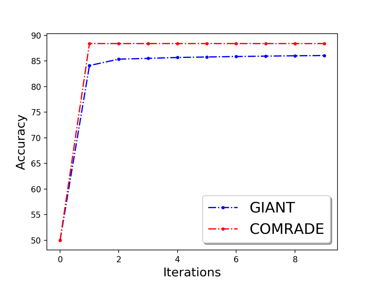
Figure 1: (First row) Comparison of training accuracy between COMRADE(Algorithm 1) and GIANT [34] with (a) w5a (b) a9a (c) Epsilon (d) Covtype dataset. (Second row) Training accuracy of (e) GIANT for ‘flipped label’ and (f) ‘negative update’ attack; and comparison of Robust GIANT and COMRADE with a9a dataset for (g) ‘flipped label’ and (h) ‘negative update’ attack.

6 Experimental Results

In this section we validate our algorithm, COMRADE in Byzantine and non-Byzantine setup on synthetically generated and benchmark LIBSVM [5] data-set. The experiments focus on the standard logistic regression problem. The logistic regression objective is defined as 1n​∑i=1nlog⁡(1+exp⁡(−yi​𝐱i⊤​𝐰))+λ2​n​‖𝐰‖2\frac{1}{n}\sum_{i=1}^{n}\log\left(1+\exp(-y_{i}\mathbf{x}_{i}^{\top}\mathbf{w})\right)+\frac{\lambda}{2n}\|\mathbf{w}\|^{2}, where 𝐰∈ℝd\mathbf{w}\in\mathbb{R}^{d} is the parameter, {𝐱i}i=1n∈ℝd\{\mathbf{x}_{i}\}_{i=1}^{n}\in\mathbb{R}^{d} are the feature data and {yi}i=1n∈{0,1}\{y_{i}\}_{i=1}^{n}\in\{0,1\} are the corresponding labels. We use ‘mpi4py’ package in distributed computing framework (swarm2) at the University of Massachusetts Amherst [31]. We choose ‘a9a’ (d=123,n≈32d=123,n\approx 32K), ‘w5a’ (d=300,n≈10​kd=300,n\approx 10k), ‘Epsilon’ (d=2000,n=0.4d=2000,n=0.4M) and ‘covtype.binary’ (d=54,n≈0.5d=54,n\approx 0.5M) classification datasets and partition the data in 2020 different worker machines. In the experiments, we choose two types of Byzantine attacks : (1). ‘flipped label’-attack where (for binary classification) the Byzantine worker machines flip the labels of the data, thus making the model learn with wrong labels, and (2). ‘negative update attack’ where the Byzantine worker machines compute the local update (𝐩^i\hat{\mathbf{p}}_{i}) and communicate −c×𝐩^i-c\times\hat{\mathbf{p}}_{i} with c∈(0,1)c\in(0,1) making the updates to be opposite of actual direction. We choose β=α+2m\beta=\alpha+\frac{2}{m}.

Refer to caption
(a) w5a
Refer to caption
(b) a9a
Refer to caption
(c) Epsilon
Refer to caption
(d) covtype
Refer to caption
(e) w5a
Refer to caption
(f) a9a
Refer to caption
(g) Epsilon
Refer to caption
(h) covtype
Refer to caption
(i) w5a ‘flipped’
Refer to caption
(j) w5q ‘negative’
Refer to caption
(k) a9a ‘flipped’
Refer to caption
(l) a9a ‘negative’
Figure 2: (First row) Accuracy of COMRADE with 10%,15%,20%10\%,15\%,20\% Byzantine workers with ‘negative update’ attack for (a). w5a (b). a9a (c). covtype (d). Epsilon. (Second row) COMRADE accuracy with 10%,15%,20%10\%,15\%,20\% Byzantine workers with ‘flipped label’ attack for (e) w5a (f) a9a (g) covtype (h) Epsilon. (Third row) Accuracy of COMRADE with ρ\rho-approximate compressor (Section 5) with 10%,15%,20%10\%,15\%,20\% Byzantine workers; (i) ‘flipped label’ attack for w5a (j) ‘negative update’ attack for w5a. (k) ‘flipped label’ attack for a9a . (l) ‘negative update’ attack for a9a dataset.

In Figure 1(first row) we compare COMRADE in non-Byzantine setup (α=β=0\alpha=\beta=0) with the state-of the art algorithm GIANT [34]. It is evident from the plot that despite the fact that COMRADE requires less communication, the algorithm is able to achieve similar accuracy. Also, we show the ineffectiveness of GIANT in the presence of Byzantine attacks. In Figure  2((e),(f)) we show the accuracy for flipped label and negative update attacks. These plots are an indicator of the requirement of robustness in the learning algorithm. So we device ‘Robust GIANT’, which is GIANT algorithm with added ‘norm based thresholding’ for robustness. In particular, we trim the worker machines based on the local gradient norm in the first round of communication of GIANT. Subsequently, in the second round of communication, the non-trimmed worker machines send the updates (product of local Hessian inverse and the local gradient) to the center machine. We compare COMRADE with ‘Robust GIANT’ in Figure 1((g),(h)) with 10%10\% Byzantine worker machines for ‘a9a’ dataset. It is evident plot that COMRADE performs better than the ‘Robust GIANT’.

Next we show the accuracy of COMRADE with different numbers of Byzantine worker machines. Here we choose c=0.9c=0.9. We show the accuracy for ’negetive update ’ attack in Figure 2(first row) and ’flipped label’ attack in Figure 2 (second row). Furthermore, we show that COMRADE works even when ρ\rho-approximate compressor is applied to the updates. In Figure  2(Third row) we plot the tranning accuracies. For compression we apply the scheme known as QSGD [1]. Further experiments can be found in the supplementary material.

7 Conclusion and Future Work

In this paper, we address the issue of communication efficiency and Byzantine robustness via second order optimization and norm based thresholding respectively for strongly convex loss. Extending our setting to handle weakly convex and non-convex loss is of immediate interest. We would also like to exploit local averaging with second order optimization. Moreover, an import aspect, privacy, is not addressed in this work. We keep this as our future research direction.

References

  • [1] D. Alistarh, D. Grubic, J. Li, R. Tomioka, and M. Vojnovic. Qsgd: Communication-efficient sgd via gradient quantization and encoding. In Advances in Neural Information Processing Systems, pages 1709–1720, 2017.
  • [2] J. Bernstein, Y.-X. Wang, K. Azizzadenesheli, and A. Anandkumar. signsgd: Compressed optimisation for non-convex problems. arXiv preprint arXiv:1802.04434, 2018.
  • [3] J. Bernstein, J. Zhao, K. Azizzadenesheli, and A. Anandkumar. signsgd with majority vote is communication efficient and byzantine fault tolerant. arXiv preprint arXiv:1810.05291, 2018.
  • [4] P. Blanchard, E. M. E. Mhamdi, R. Guerraoui, and J. Stainer. Byzantine-tolerant machine learning. arXiv preprint arXiv:1703.02757, 2017.
  • [5] C.-C. Chang and C.-J. Lin. Libsvm: A library for support vector machines. ACM transactions on intelligent systems and technology (TIST), 2(3):27, 2011.
  • [6] Y. Chen, L. Su, and J. Xu. Distributed statistical machine learning in adversarial settings: Byzantine gradient descent. Proceedings of the ACM on Measurement and Analysis of Computing Systems, 1(2):44, 2017.
  • [7] R. Crane and F. Roosta. Dingo: Distributed newton-type method for gradient-norm optimization. In Advances in Neural Information Processing Systems, pages 9494–9504, 2019.
  • [8] G. Damaskinos, E. M. El Mhamdi, R. Guerraoui, A. H. A. Guirguis, and S. L. A. Rouault. Aggregathor: Byzantine machine learning via robust gradient aggregation. page 19, 2019. Published in the Conference on Systems and Machine Learning (SysML) 2019, Stanford, CA, USA.
  • [9] M. Derezinski and M. W. Mahoney. Distributed estimation of the inverse hessian by determinantal averaging. In Advances in Neural Information Processing Systems, pages 11401–11411, 2019.
  • [10] J. Devlin, M.-W. Chang, K. Lee, and K. Toutanova. BERT: Pre-training of deep bidirectional transformers for language understanding. arXiv preprint arXiv:1810.04805, 2018.
  • [11] P. Drineas, M. Magdon-Ismail, M. W. Mahoney, and D. P. Woodruff. Fast approximation of matrix coherence and statistical leverage. Journal of Machine Learning Research, 13(Dec):3475–3506, 2012.
  • [12] P. Drineas and M. W. Mahoney. Randnla: randomized numerical linear algebra. Communications of the ACM, 59(6):80–90, 2016.
  • [13] J. Feng, H. Xu, and S. Mannor. Distributed robust learning. arXiv preprint arXiv:1409.5937, 2014.
  • [14] V. Gandikota, R. K. Maity, and A. Mazumdar. vqsgd: Vector quantized stochastic gradient descent. arXiv preprint arXiv:1911.07971, 2019.
  • [15] A. Ghosh, J. Hong, D. Yin, and K. Ramchandran. Robust federated learning in a heterogeneous environment. arXiv preprint arXiv:1906.06629, 2019.
  • [16] A. Ghosh, R. K. Maity, S. Kadhe, A. Mazumdar, and K. Ramchandran. Communication-efficient and byzantine-robust distributed learning. arXiv preprint arXiv:1911.09721, 2019.
  • [17] A. Ghosh, R. K. Maity, A. Mazumdar, and K. Ramchandran. Communication efficient distributed approximate newton method. ISIT 2020 (accepted), https://tinyurl.com/ujnpt4c, 2020.
  • [18] V. Gupta, S. Kadhe, T. Courtade, M. W. Mahoney, and K. Ramchandran. Oversketched newton: Fast convex optimization for serverless systems. arXiv preprint arXiv:1903.08857, 2019.
  • [19] S. P. Karimireddy, Q. Rebjock, S. U. Stich, and M. Jaggi. Error feedback fixes signsgd and other gradient compression schemes. arXiv preprint arXiv:1901.09847, 2019.
  • [20] J. Konečnỳ, H. B. McMahan, D. Ramage, and P. Richtárik. Federated optimization: Distributed machine learning for on-device intelligence. arXiv preprint arXiv:1610.02527, 2016.
  • [21] L. Lamport, R. Shostak, and M. Pease. The byzantine generals problem. ACM Trans. Program. Lang. Syst., 4(3):382–401, July 1982.
  • [22] M. W. Mahoney. Randomized algorithms for matrices and data. Foundations and Trends® in Machine Learning, 3(2):123–224, 2011.
  • [23] E. M. E. Mhamdi, R. Guerraoui, and S. Rouault. The hidden vulnerability of distributed learning in byzantium. arXiv preprint arXiv:1802.07927, 2018.
  • [24] M. Pilanci and M. J. Wainwright. Newton sketch: A near linear-time optimization algorithm with linear-quadratic convergence. SIAM Journal on Optimization, 27(1):205–245, 2017.
  • [25] S. J. Reddi, J. Konečnỳ, P. Richtárik, B. Póczós, and A. Smola. Aide: Fast and communication efficient distributed optimization. arXiv preprint arXiv:1608.06879, 2016.
  • [26] F. Roosta, Y. Liu, P. Xu, and M. W. Mahoney. Newton-mr: Newton’s method without smoothness or convexity. arXiv preprint arXiv:1810.00303, 2018.
  • [27] O. Shamir, N. Srebro, and T. Zhang. Communication-efficient distributed optimization using an approximate newton-type method. In International conference on machine learning, pages 1000–1008, 2014.
  • [28] S. U. Stich, J.-B. Cordonnier, and M. Jaggi. Sparsified sgd with memory. In Advances in Neural Information Processing Systems, pages 4447–4458, 2018.
  • [29] L. Su and N. H. Vaidya. Fault-tolerant multi-agent optimization: optimal iterative distributed algorithms. In Proceedings of the 2016 ACM symposium on principles of distributed computing, pages 425–434. ACM, 2016.
  • [30] A. T. Suresh, F. X. Yu, S. Kumar, and H. B. McMahan. Distributed mean estimation with limited communication. In Proceedings of the 34th International Conference on Machine Learning-Volume 70, pages 3329–3337. JMLR. org, 2017.
  • [31] Swarm2. Swarm user documentation. https://people.cs.umass.edu/˜swarm/index.php?n=Main.NewSwarmDoc, 2018. Accessed: 2018-01-05.
  • [32] H. Wang, S. Sievert, S. Liu, Z. Charles, D. Papailiopoulos, and S. Wright. Atomo: Communication-efficient learning via atomic sparsification. In Advances in Neural Information Processing Systems, pages 9850–9861, 2018.
  • [33] S. Wang, A. Gittens, and M. W. Mahoney. Sketched ridge regression: Optimization perspective, statistical perspective, and model averaging. The Journal of Machine Learning Research, 18(1):8039–8088, 2017.
  • [34] S. Wang, F. Roosta, P. Xu, and M. W. Mahoney. Giant: Globally improved approximate newton method for distributed optimization. In Advances in Neural Information Processing Systems, pages 2332–2342, 2018.
  • [35] W. Wen, C. Xu, F. Yan, C. Wu, Y. Wang, Y. Chen, and H. Li. Terngrad: Ternary gradients to reduce communication in distributed deep learning. In Advances in neural information processing systems, pages 1509–1519, 2017.
  • [36] D. Yin, Y. Chen, R. Kannan, and P. Bartlett. Byzantine-robust distributed learning: Towards optimal statistical rates. In J. Dy and A. Krause, editors, Proceedings of the 35th International Conference on Machine Learning, volume 80 of Proceedings of Machine Learning Research, pages 5650–5659, StockholmsmÀssan, Stockholm Sweden, 10–15 Jul 2018. PMLR.
  • [37] D. Yin, Y. Chen, R. Kannan, and P. Bartlett. Defending against saddle point attack in Byzantine-robust distributed learning. In K. Chaudhuri and R. Salakhutdinov, editors, Proceedings of the 36th International Conference on Machine Learning, volume 97 of Proceedings of Machine Learning Research, pages 7074–7084, Long Beach, California, USA, 09–15 Jun 2019. PMLR.
  • [38] Y. Zhang and X. Lin. Disco: Distributed optimization for self-concordant empirical loss. In International conference on machine learning, pages 362–370, 2015.

Appendix

8 Appendix A: Analysis of Section 3

Matrix Sketching
Here we briefly discuss the matrix sketching that is broadly used in the context of randomized linear algebra. For any matrix 𝐀∈ℝn×d\mathbf{A}\in\mathbb{R}^{n\times d} the sketched matrix 𝐙∈ℝs×d\mathbf{Z}\in\mathbb{R}^{s\times d} is defined as 𝐒T​𝐀\mathbf{S}^{T}\mathbf{A} where 𝐒∈ℝn×s\mathbf{S}\in\mathbb{R}^{n\times s} is the sketching matrix (typically s<ns<n). Based on the scope and basis of the application, the sketched matrix is constructed by taking linear combination of the rows of matrix which is known as random projection or by sampling and scaling a subset of the rows of the matrix which is known as random sampling. The sketching is done to get a smaller representation of the original matrix to reduce computational cost.

Here we consider a uniform row sampling scheme. The matrix 𝐙\mathbf{Z} is formed by sampling and scaling rows of the matrix 𝐀\mathbf{A}. Each row of the matrix 𝐀\mathbf{A} is sampled with probability p=1np=\frac{1}{n} and scaled by multiplying with 1s​p\frac{1}{\sqrt{sp}} .

ℙ⁡(𝐳i=𝐚js​p)=p,\displaystyle\mathbb{P}\left(\mathbf{z}_{i}=\frac{\mathbf{a}_{j}}{\sqrt{sp}}\right)=p,

where 𝐳i\mathbf{z}_{i} is the ii-th row matrix 𝐙\mathbf{Z} and 𝐚j\mathbf{a}_{j} is the jj th row of the matrix 𝐀\mathbf{A}. Consequently the sketching matrix 𝐒\mathbf{S} has one non-zero entry in each column.

We define the matrix 𝐀t⊤=[𝐚1⊤,…,𝐚n⊤]∈ℝd×n\mathbf{A}_{t}^{\top}=[\mathbf{a}_{1}^{\top},\ldots,\mathbf{a}_{n}^{\top}]\in\mathbb{R}^{d\times n} where 𝐚j=ℓj′′​(𝐰⊤​𝐱j)​𝐱j\mathbf{a}_{j}=\sqrt{\ell^{\prime\prime}_{j}(\mathbf{w}^{\top}\mathbf{x}_{j})}\,\mathbf{x}_{j}. So the exact Hessian in equation (2) is 𝐇t=1n​𝐀t⊤​𝐀t+λ​𝐈\mathbf{H}_{t}=\frac{1}{n}\mathbf{A}_{t}^{\top}\mathbf{A}_{t}+\lambda\mathbf{I}. Assume that SiS_{i} is the set of features that are held by the iith worker machine. So the local Hessian is

𝐇i,t=1s​∑j∈Siℓj′′​(𝐰⊤​𝐱j)​𝐱j​𝐱j⊤+λ​𝐈=1s​𝐀i,t⊤​𝐀i,t+λ​𝐈,\displaystyle\mathbf{H}_{i,t}=\frac{1}{s}\sum_{j\in S_{i}}\ell^{\prime\prime}_{j}(\mathbf{w}^{\top}\mathbf{x}_{j})\mathbf{x}_{j}\mathbf{x}_{j}^{\top}+\lambda\mathbf{I}=\frac{1}{s}\mathbf{A}_{i,t}^{\top}\mathbf{A}_{i,t}+\lambda\mathbf{I},

where 𝐀i,t∈ℝs×d\mathbf{A}_{i,t}\in\mathbb{R}^{s\times d} and the row of the matrix 𝐀i,t\mathbf{A}_{i,t} is indexed by SiS_{i}. Also we define 𝐁t=[𝐛1,…,𝐛n]∈ℝd×n\mathbf{B}_{t}=[\mathbf{b}_{1},\ldots,\mathbf{b}_{n}]\in\mathbb{R}^{d\times n} where 𝐛i=ℓi′​(𝐰⊤​𝐱i)​𝐱i\mathbf{b}_{i}=\ell^{\prime}_{i}(\mathbf{w}^{\top}\mathbf{x}_{i})\mathbf{x}_{i}. So the exact gradient in equation (2) is 𝐠t=1n​𝐁t​𝟏+λ​𝐰t\mathbf{g}_{t}=\frac{1}{n}\mathbf{B}_{t}\mathbf{1}+\lambda\mathbf{w}_{t} and the local gradient is

𝐠i,t=1s​∑i∈Siℓj′​(𝐰t⊤​𝐱i)​𝐱i+λ​𝐰t=1s​𝐁i,t​𝟏+λ​𝐰t,\displaystyle\mathbf{g}_{i,t}=\frac{1}{s}\sum_{i\in S_{i}}\ell_{j}^{\prime}(\mathbf{w}_{t}^{\top}\mathbf{x}_{i})\mathbf{x}_{i}+\lambda\mathbf{w}_{t}=\frac{1}{s}\mathbf{B}_{i,t}\mathbf{1}+\lambda\mathbf{w}_{t},

where 𝐁i,t\mathbf{B}_{i,t} is the matrix with column indexed by SiS_{i}. If {𝐒i}i=1m\{\mathbf{S}_{i}\}_{i=1}^{m} are the sketching matrices then the local Hessian and gradient can be expressed as

𝐇i,t=𝐀t⊤​𝐒i​𝐒i⊤​𝐀t⊤+λ​𝐈\displaystyle\mathbf{H}_{i,t}=\mathbf{A}_{t}^{\top}\mathbf{S}_{i}\mathbf{S}_{i}^{\top}\mathbf{A}_{t}^{\top}+\lambda\mathbf{I} 𝐠i,t=1n​𝐁𝐒i​𝐒i⊤​𝟏+λ​𝐰.\displaystyle\mathbf{g}_{i,t}=\frac{1}{n}\mathbf{B}\mathbf{S}_{i}\mathbf{S}_{i}^{\top}\mathbf{1}+\lambda\mathbf{w}. (9)

With the help of sketching idea later we show that the local hessian and gradient are close to the exact hessian and gradient.

The Quadratic function For the purpose of analysis we define an auxiliary quadratic function

ϕ⁡(𝐩)=12​𝐩⊤​𝐇t​𝐩−𝐠t⊤​𝐩=12​𝐩⊤​(𝐀t⊤​𝐀t+λ​𝐈)​𝐩−𝐠t⊤​𝐩.\displaystyle\phi(\mathbf{p})=\frac{1}{2}\mathbf{p}^{\top}\mathbf{H}_{t}\mathbf{p}-\mathbf{g}_{t}^{\top}\mathbf{p}=\frac{1}{2}\mathbf{p}^{\top}(\mathbf{A}_{t}^{\top}\mathbf{A}_{t}+\lambda\mathbf{I})\mathbf{p}-\mathbf{g}_{t}^{\top}\mathbf{p}. (10)

The optimal solution to the above function is

𝐩∗=arg⁡min⁡ϕ⁡(𝐩)=𝐇t−1​𝐠t=(𝐀t⊤​𝐀t+λ​𝐈)−1​𝐠t,\displaystyle\mathbf{p}^{*}=\arg\min\phi(\mathbf{p})=\mathbf{H}_{t}^{-1}\mathbf{g}_{t}=(\mathbf{A}_{t}^{\top}\mathbf{A}_{t}+\lambda\mathbf{I})^{-1}\mathbf{g}_{t},

which is also the optimal direction of the global Newton update. In this work we consider the local and global (approximate ) Newton direction to be

𝐩^i,t=(𝐀⊤​𝐒i​𝐒i⊤​𝐀+λ​𝐈)−1​𝐠i,t,𝐩^t=1m​∑i=1m𝐩^i,t.\displaystyle\hat{\mathbf{p}}_{i,t}=(\mathbf{A}^{\top}\mathbf{S}_{i}\mathbf{S}_{i}^{\top}\mathbf{A}+\lambda\mathbf{I})^{-1}\mathbf{g}_{i,t},\quad\hat{\mathbf{p}}_{t}=\frac{1}{m}\sum_{i=1}^{m}\hat{\mathbf{p}}_{i,t}.

respectively. And it can be easily verified that each local update 𝐩^i,t\hat{\mathbf{p}}_{i,t} is optimal solution to the following quadratic function

ϕ^i,t​(p)=12​𝐩⊤​(𝐀⊤​𝐒i​𝐒i⊤​𝐀+λ​𝐈)​𝐩−𝐠i⊤​𝐩.\displaystyle\hat{\phi}_{i,t}(p)=\frac{1}{2}\mathbf{p}^{\top}(\mathbf{A}^{\top}\mathbf{S}_{i}\mathbf{S}_{i}^{\top}\mathbf{A}+\lambda\mathbf{I})\mathbf{p}-\mathbf{g}_{i}^{\top}\mathbf{p}. (11)

In our convergence analysis we show that value of the quadratic function in (10) with value 𝐩^t\hat{\mathbf{p}}_{t} is close to the optimal value.

Singular Value Decomposition (SVD) For any matrix 𝐀∈ℝn×d\mathbf{A}\in\mathbb{R}^{n\times d} with rank rr, the singular value decomposition is defined as 𝐀=𝐔​𝚺​𝐕⊤\mathbf{A}=\mathbf{U}\mathbf{\Sigma}\mathbf{V}^{\top} where 𝐔,𝐕\mathbf{U},\mathbf{V} are n×rn\times r and d×rd\times r column orthogonal matrices respectively and 𝚺\mathbf{\Sigma} is a r×rr\times r diagonal matrix with diagonal entries {σ1,…​σr}\{\sigma_{1},\ldots\sigma_{r}\}. If 𝐀\mathbf{A} is a symmetric positive semi-definite matrix then 𝐔=𝐕\mathbf{U}=\mathbf{V}.

8.1 Analysis

Lemma 1 (McDiarmid’s Inequality).

Let X=X1,…,XmX=X_{1},\ldots,X_{m} be mm independent random variables taking values from some set AA, and assume that f:Am→ℝf:A^{m}\rightarrow\mathbb{R} satisfies the following condition (bounded differences ):

supx1,…,xm,x^i|f⁡(xi,…,xi,…,xm)−f⁡(xi,…,x^i,…,xm)|≤ci,\displaystyle\sup_{x_{1},\ldots,x_{m},\hat{x}_{i}}\left|f(x_{i},\ldots,x_{i},\ldots,x_{m})-f(x_{i},\ldots,\hat{x}_{i},\ldots,x_{m})\right|\leq c_{i},

for all i∈{1,…,m}i\in\{1,\ldots,m\}. Then for any ϵ>0\epsilon>0 we have

P[f(X1,…,Xm)−𝔼[f(X1,…,Xm)]≥ϵ]≤exp(−2​ϵ2∑i=1mci2).\displaystyle P\left[f(X_{1},\ldots,X_{m})-\mathbb{E}[f(X_{1},\ldots,X_{m})]\geq\epsilon\right]\leq\exp\left(-\frac{2\epsilon^{2}}{\sum_{i=1}^{m}c_{i}^{2}}\right).

The property described in the following Lemma 2 is a very useful result for uniform row sampling sketching matrix.

Lemma 2 (Lemma 8 [34]).

Let η,δ∈(0,1)\eta,\delta\in(0,1) be a fixed parameter and r=rank​(𝐀t)r=\text{rank}(\mathbf{A}_{t}) and 𝐔∈ℝn×r\mathbf{U}\in\mathbb{R}^{n\times r} be the orthonormal bases of the matrix 𝐀t\mathbf{A}_{t}. Let {𝐒i}i=1m\{\mathbf{S}_{i}\}_{i=1}^{m} be sketching matrices and 𝐒=1m​[𝐒1,…​𝐒m]∈ℝn×m​s\mathbf{S}=\frac{1}{\sqrt{m}}[\mathbf{S}_{1},\ldots\mathbf{S}_{m}]\in\mathbb{R}^{n\times ms}. With probability 1−δ1-\delta the following holds

‖𝐔⊤​𝐒i​𝐒i⊤​𝐔−𝐈‖2≤η∀i∈[m] and ‖𝐔⊤​𝐒𝐒⊤​𝐔−𝐈‖2≤ηm.\displaystyle\left\|\mathbf{U}^{\top}\mathbf{S}_{i}\mathbf{S}_{i}^{\top}\mathbf{U}-\mathbf{I}\right\|_{2}\leq\eta\quad\forall i\in[m]\quad\text{ and }\quad\left\|\mathbf{U}^{\top}\mathbf{S}\mathbf{S}^{\top}\mathbf{U}-\mathbf{I}\right\|_{2}\leq\frac{\eta}{\sqrt{m}}.
Lemma 3.

Let 𝐒∈ℝn×s\mathbf{S}\in\mathbb{R}^{n\times s} be any uniform sampling sketching matrix, then for any matrix 𝐁=[𝐛1,…,𝐛n]∈ℝd×n\mathbf{B}=[\mathbf{b}_{1},\ldots,\mathbf{b}_{n}]\in\mathbb{R}^{d\times n} with probability 1−δ1-\delta for any δ>0\delta>0 we have,

‖1n​𝐁𝐒𝐒⊤​𝟏−1n​𝐁𝟏‖≤(1+2​ln⁡(1δ))​1s​maxi​‖𝐛i‖,\displaystyle\|\frac{1}{n}\mathbf{B}\mathbf{S}\mathbf{S}^{\top}\mathbf{1}-\frac{1}{n}\mathbf{B}\mathbf{1}\|\leq(1+\sqrt{2\ln(\frac{1}{\delta})})\sqrt{\frac{1}{s}}\max_{i}\|\mathbf{b}_{i}\|,

where 𝟏\mathbf{1} is all ones vector.

Proof.

The vector 𝐁𝟏\mathbf{B}\mathbf{1} is the sum of column of the matrix 𝐁\mathbf{B} and 𝐁𝐒𝐒⊤​𝟏\mathbf{B}\mathbf{S}\mathbf{S}^{\top}\mathbf{1} is the sum of uniformly sampled and scaled column of the matrix 𝐁\mathbf{B} where the scaling factor is 1s​p\frac{1}{\sqrt{sp}} with p=1np=\frac{1}{n}. If (i1,…,is)(i_{1},\ldots,i_{s}) is the set of sampled indices then 𝐁𝐒𝐒⊤​𝟏=∑k∈(i1,…,is)1s​p​𝐛k\mathbf{B}\mathbf{S}\mathbf{S}^{\top}\mathbf{1}=\sum_{k\in(i_{1},\ldots,i_{s})}\frac{1}{sp}\mathbf{b}_{k}.

Define the function f⁡(i1,…,is)=‖1n​𝐁𝐒𝐒⊤​𝟏−1n​𝐁𝟏‖f(i_{1},\ldots,i_{s})=\|\frac{1}{n}\mathbf{B}\mathbf{S}\mathbf{S}^{\top}\mathbf{1}-\frac{1}{n}\mathbf{B}\mathbf{1}\|. Now consider a sampled set (i1,…,ij′,…,is)(i_{1},\ldots,i_{j^{\prime}},\ldots,i_{s}) with only one item (column) replaced then the bounded difference is

Δ\displaystyle\Delta =|f⁡(i1,…,ij,…,is)−f⁡(i1,…,ij′,…,is)|\displaystyle=|f(i_{1},\ldots,i_{j},\ldots,i_{s})-f(i_{1},\ldots,i_{j^{\prime}},\ldots,i_{s})|
=|1n​‖1s​p​𝐛ij′−1s​p​𝐛ij‖|≤2s​maxi​‖𝐛i‖.\displaystyle=|\frac{1}{n}\|\frac{1}{sp}\mathbf{b}_{i_{j}^{\prime}}-\frac{1}{sp}\mathbf{b}_{i_{j}}\||\leq\frac{2}{s}\max_{i}\|\mathbf{b}_{i}\|.

Now we have the expectation

𝔼⁡[‖1n​𝐁𝐒𝐒⊤​𝟏−1n​𝐁𝟏‖2]\displaystyle\mathbb{E}[\|\frac{1}{n}\mathbf{B}\mathbf{S}\mathbf{S}^{\top}\mathbf{1}-\frac{1}{n}\mathbf{B}\mathbf{1}\|^{2}] ≤ns​n2​∑i=1n‖𝐛i‖2=1s​maxi​‖𝐛i‖2\displaystyle\leq\frac{n}{sn^{2}}\sum_{i=1}^{n}\|\mathbf{b}_{i}\|^{2}=\frac{1}{s}\max_{i}\|\mathbf{b}_{i}\|^{2}
⇒𝔼⁡[‖1n​𝐁𝐒𝐒⊤​𝟏−1n​𝐁𝟏‖]\displaystyle\Rightarrow\mathbb{E}[\|\frac{1}{n}\mathbf{B}\mathbf{S}\mathbf{S}^{\top}\mathbf{1}-\frac{1}{n}\mathbf{B}\mathbf{1}\|] ≤1s​maxi​‖𝐛i‖.\displaystyle\leq\sqrt{\frac{1}{s}}\max_{i}\|\mathbf{b}_{i}\|.

Using McDiarmid inequality (Lemma 1) we have

P[‖1n𝐁𝐒𝐒⊤𝟏−1n𝐁𝟏∥≥1smaxi∥𝐛i∥+t]≤exp(−2​t2s​Δ2).\displaystyle P[\left\|\frac{1}{n}\mathbf{B}\mathbf{S}\mathbf{S}^{\top}\mathbf{1}-\frac{1}{n}\mathbf{B}\mathbf{1}\|\geq\sqrt{\frac{1}{s}}\max_{i}\|\mathbf{b}_{i}\|+t\right]\leq\exp\left(-\frac{2t^{2}}{s\Delta^{2}}\right).

Equating the probability with δ\delta we have

exp⁡(−2​t2s​Δ2)=δ\displaystyle\exp(-\frac{2t^{2}}{s\Delta^{2}})=\delta
⇒\displaystyle\Rightarrow t=Δ​s2​ln⁡(1δ)=maxi⁡‖𝐛i‖​2s​ln⁡(1δ).\displaystyle t=\Delta\sqrt{\frac{s}{2}\ln(\frac{1}{\delta})}=\max_{i}\|\mathbf{b}_{i}\|\sqrt{\frac{2}{s}\ln(\frac{1}{\delta})}.

Finally we have with probability 1−δ1-\delta

‖1n​𝐁𝐒𝐒⊤​𝟏−1n​𝐁𝟏‖≤(1+2​ln⁡(1δ))​1s​maxi​‖𝐛i‖.\displaystyle\|\frac{1}{n}\mathbf{B}\mathbf{S}\mathbf{S}^{\top}\mathbf{1}-\frac{1}{n}\mathbf{B}\mathbf{1}\|\leq(1+\sqrt{2\ln(\frac{1}{\delta})})\sqrt{\frac{1}{s}}\max_{i}\|\mathbf{b}_{i}\|.

∎

Remark 8.

For mm sketching matrix {𝐒i}i=1m\{\mathbf{S}_{i}\}_{i=1}^{m}, the bound in the Lemma 3 is

‖1n​𝐁𝐒i​𝐒i⊤​𝟏−1n​𝐁𝟏‖≤(1+2​ln⁡(mδ))​1s​maxi​‖𝐛i‖,\displaystyle\|\frac{1}{n}\mathbf{B}\mathbf{S}_{i}\mathbf{S}_{i}^{\top}\mathbf{1}-\frac{1}{n}\mathbf{B}\mathbf{1}\|\leq(1+\sqrt{2\ln(\frac{m}{\delta})})\sqrt{\frac{1}{s}}\max_{i}\|\mathbf{b}_{i}\|,

with probability 1−δ1-\delta for any δ>0\delta>0 for all i∈{1,2,…,m}i\in\{1,2,\ldots,m\}. In the case that each worker machine holds data based on the uniform sketching matrix the local gradient is close to the exact gradient. Thus the local second order update acts as a good approximate to the exact Netwon update.

Now we consider the update rule of GIANT [34] where the update is done in two rounds in each iteration. In the first round each worker machine computes and send the local gradient and the center machine computes the exact gradient 𝐠t\mathbf{g}_{t} in iteration tt. Next the center machine broadcasts the exact gradient and each worker machine computes the local Hessian and send 𝐩~i,t=(𝐇i,t)−1​𝐠t\tilde{\mathbf{p}}_{i,t}=(\mathbf{H}_{i,t})^{-1}\mathbf{g}_{t} to the center machine and the center machine computes the approximate Newton direction 𝐩~t=1m​∑i=1m𝐩~i,t\tilde{\mathbf{p}}_{t}=\frac{1}{m}\sum_{i=1}^{m}\tilde{\mathbf{p}}_{i,t}. Now based on this we restate the following lemma (Lemma 6 [34]).

Lemma 4.

Let {𝐒i}i=1m∈ℝn×s\{\mathbf{S}_{i}\}_{i=1}^{m}\in\mathbb{R}^{n\times s} be sketching matrices based on Lemma 2. Let ϕt\phi_{t} be defined in (10) and 𝐩~t\tilde{\mathbf{p}}_{t} be the update. It holds that

min𝐩⁡ϕt​(𝐩)≤ϕt​(𝐩~t)≤(1−ζ2)​min𝐩​ϕt​(𝐩),\displaystyle\min_{\mathbf{p}}\phi_{t}(\mathbf{p})\leq\phi_{t}(\tilde{\mathbf{p}}_{t})\leq(1-\zeta^{2})\min_{\mathbf{p}}\phi_{t}(\mathbf{p}),

where ζ=ν⁡(ηm+η21−η)\zeta=\nu(\frac{\eta}{\sqrt{m}}+\frac{\eta^{2}}{1-\eta}) and ν=σm​a​x​(𝐀⊤​𝐀)σm​a​x​(𝐀⊤​𝐀)+n​λ≤1\nu=\frac{\sigma_{max}(\mathbf{A}^{\top}\mathbf{A})}{\sigma_{max}(\mathbf{A}^{\top}\mathbf{A})+n\lambda}\leq 1.

Now we prove similar guarantee for the update according to COMRADE in Algorithm 1.

Lemma 5.

Let {𝐒i}i=1m∈ℝn×s\{\mathbf{S}_{i}\}_{i=1}^{m}\in\mathbb{R}^{n\times s} be sketching matrices based on Lemma 2. Let ϕt\phi_{t} be defined in (10) and 𝐩^t\hat{\mathbf{p}}_{t} be defined in Algorithm 1(β=0\beta=0)

min𝐩⁡ϕt​(𝐩)≤ϕt​(𝐩^t)≤ϵ2+(1−ζ2)​min𝐩​ϕt​(𝐩),\displaystyle\min_{\mathbf{p}}\phi_{t}(\mathbf{p})\leq\phi_{t}(\hat{\mathbf{p}}_{t})\leq\epsilon^{2}+(1-\zeta^{2})\min_{\mathbf{p}}\phi_{t}(\mathbf{p}),

where ϵ=11−η​1σm​i​n​(𝐇t)​(1+2​ln⁡(mδ))​1s​maxi​‖𝐛i‖\epsilon=\frac{1}{1-\eta}\frac{1}{\sqrt{\sigma_{min}(\mathbf{H}_{t})}}(1+\sqrt{2\ln(\frac{m}{\delta})})\sqrt{\frac{1}{s}}\max_{i}\|\mathbf{b}_{i}\| and ζ=ν⁡(ηm+η21−η)\zeta=\nu(\frac{\eta}{\sqrt{m}}+\frac{\eta^{2}}{1-\eta}) and ν=σm​a​x​(𝐀⊤​𝐀)σm​a​x​(𝐀⊤​𝐀)+n​λ\nu=\frac{\sigma_{max}(\mathbf{A}^{\top}\mathbf{A})}{\sigma_{max}(\mathbf{A}^{\top}\mathbf{A})+n\lambda}.

Proof.

First consider the quadratic function (10)

ϕt​(𝐩^t)−ϕt​(𝐩∗)\displaystyle\phi_{t}(\hat{\mathbf{p}}_{t})-\phi_{t}(\mathbf{p}^{*}) =12​‖𝐇t12​(𝐩^t−𝐩∗)‖2\displaystyle=\frac{1}{2}\|\mathbf{H}_{t}^{\frac{1}{2}}(\hat{\mathbf{p}}_{t}-\mathbf{p}^{*})\|^{2}
≤(‖𝐇t12​(𝐩^t−𝐩~t)‖2CLOSE⏟T​e​r​m​1+OPEN‖𝐇t12​(𝐩~t−𝐩∗)‖)2⏟T​e​r​m​2,\displaystyle\leq\underbrace{(\|\mathbf{H}_{t}^{\frac{1}{2}}(\hat{\mathbf{p}}_{t}-\tilde{\mathbf{p}}_{t})\|^{2}}_{Term1}+\underbrace{\|\mathbf{H}_{t}^{\frac{1}{2}}(\tilde{\mathbf{p}}_{t}-\mathbf{p}^{*})\|)^{2}}_{Term2}, (12)

where 𝐩~t=1m​∑i=1m(𝐇i,t)−1​𝐠t\tilde{\mathbf{p}}_{t}=\frac{1}{m}\sum_{i=1}^{m}(\mathbf{H}_{i,t})^{-1}\mathbf{g}_{t}. First we bound the Term 2 of (12) using the quadratic function and Lemma 4

OPEN12​‖𝐇t12​(𝐩~t−𝐩∗)‖)2\displaystyle\frac{1}{2}\left\|\mathbf{H}_{t}^{\frac{1}{2}}(\tilde{\mathbf{p}}_{t}-\mathbf{p}^{*})\right\|)^{2} ≤ζ2‖𝐇t12𝐩∗‖2 (Using Lemma 4 )\displaystyle\leq\zeta^{2}\left\|\mathbf{H}_{t}^{\frac{1}{2}}\mathbf{p}^{*}\right\|^{2}\quad\text{ (Using Lemma~\ref{lem:giant} )}
=−ζ2​ϕt​(𝐩∗).\displaystyle=-\zeta^{2}\phi_{t}(\mathbf{p}^{*}). (13)

The step in equation (13) is from the definition of the function ϕt\phi_{t} and 𝐩∗\mathbf{p}^{*}. It can be shown that

ϕt​(𝐩∗)=−‖𝐇t12​𝐩∗‖2.\displaystyle\phi_{t}(\mathbf{p}^{*})=-\left\|\mathbf{H}_{t}^{\frac{1}{2}}\mathbf{p}^{*}\right\|^{2}.

Now we bound the Term 1 in (12). By Lemma 2, we have (1−η)​𝐀t⊤​𝐀t⪯𝐀t⊤​𝐒i​𝐒i⊤​𝐀t⪯(1+η)​𝐀t⊤​𝐀t(1-\eta)\mathbf{A}_{t}^{\top}\mathbf{A}_{t}\preceq\mathbf{A}_{t}^{\top}\mathbf{S}_{i}\mathbf{S}_{i}^{\top}\mathbf{A}_{t}\preceq(1+\eta)\mathbf{A}_{t}^{\top}\mathbf{A}_{t}. Following we have (1−η)​𝐇t⪯𝐇i,t⪯(1+η)​𝐇t(1-\eta)\mathbf{H}_{t}\preceq\mathbf{H}_{i,t}\preceq(1+\eta)\mathbf{H}_{t}. Thus there exists matrix ξi\mathbf{\xi}_{i} satisfying

𝐇t12​𝐇i,t−1​𝐇t12=𝐈+ξiand −η1+η⪯ξi⪯η1−η,\displaystyle\mathbf{H}_{t}^{\frac{1}{2}}\mathbf{H}_{i,t}^{-1}\mathbf{H}_{t}^{\frac{1}{2}}=\mathbf{I}+\mathbf{\xi}_{i}\quad\text{and }\quad-\frac{\eta}{1+\eta}\preceq\mathbf{\xi}_{i}\preceq\frac{\eta}{1-\eta},

So we have,

‖𝐇t12​𝐇i,t−1​𝐇t12‖≤1+η1−η=11−η.\displaystyle\left\|\mathbf{H}_{t}^{\frac{1}{2}}\mathbf{H}_{i,t}^{-1}\mathbf{H}_{t}^{\frac{1}{2}}\right\|\leq 1+\frac{\eta}{1-\eta}=\frac{1}{1-\eta}. (14)

Now we have

‖𝐇t12​(𝐩^t−𝐩~t)‖\displaystyle\left\|\mathbf{H}_{t}^{\frac{1}{2}}(\hat{\mathbf{p}}_{t}-\tilde{\mathbf{p}}_{t})\right\| =‖𝐇t12​1m​∑i=1m(𝐩^i,t−𝐩~i,t)‖\displaystyle=\left\|\mathbf{H}_{t}^{\frac{1}{2}}\frac{1}{m}\sum_{i=1}^{m}(\hat{\mathbf{p}}_{i,t}-\tilde{\mathbf{p}}_{i,t})\right\|
≤1m​∑i=1m‖𝐇t12​(𝐩^i,t−𝐩~i,t)‖\displaystyle\leq\frac{1}{m}\sum_{i=1}^{m}\left\|\mathbf{H}_{t}^{\frac{1}{2}}(\hat{\mathbf{p}}_{i,t}-\tilde{\mathbf{p}}_{i,t})\right\|
=1m​∑i=1m‖𝐇t12​𝐇i,t−1​(𝐠i,t−𝐠t)‖\displaystyle=\frac{1}{m}\sum_{i=1}^{m}\left\|\mathbf{H}_{t}^{\frac{1}{2}}\mathbf{H}_{i,t}^{-1}(\mathbf{g}_{i,t}-\mathbf{g}_{t})\right\|
=1m​∑i=1m‖𝐇t12​𝐇i,t−1​𝐇t12​𝐇t−12​(𝐠i,t−𝐠t)‖\displaystyle=\frac{1}{m}\sum_{i=1}^{m}\left\|\mathbf{H}_{t}^{\frac{1}{2}}\mathbf{H}_{i,t}^{-1}\mathbf{H}_{t}^{\frac{1}{2}}\mathbf{H}_{t}^{-\frac{1}{2}}(\mathbf{g}_{i,t}-\mathbf{g}_{t})\right\|
≤1m​∑i=1m‖𝐇t12​𝐇i,t−1​𝐇t12‖​‖𝐇t−12​(𝐠i,t−𝐠t)‖\displaystyle\leq\frac{1}{m}\sum_{i=1}^{m}\left\|\mathbf{H}_{t}^{\frac{1}{2}}\mathbf{H}_{i,t}^{-1}\mathbf{H}_{t}^{\frac{1}{2}}\right\|\left\|\mathbf{H}_{t}^{-\frac{1}{2}}(\mathbf{g}_{i,t}-\mathbf{g}_{t})\right\|
≤11−η1m∑i=1m‖𝐇t−12(𝐠i,t−𝐠t)‖ ( Using (14))\displaystyle\leq\frac{1}{1-\eta}\frac{1}{m}\sum_{i=1}^{m}\left\|\mathbf{H}_{t}^{-\frac{1}{2}}(\mathbf{g}_{i,t}-\mathbf{g}_{t})\right\|\quad\text{ ( Using \eqref{htl2})}
≤11−η​1σm​i​n​(𝐇t)​1m​∑i=1m‖(𝐠i,t−𝐠t)‖.\displaystyle\leq\frac{1}{1-\eta}\frac{1}{\sqrt{\sigma_{min}(\mathbf{H}_{t})}}\frac{1}{m}\sum_{i=1}^{m}\left\|(\mathbf{g}_{i,t}-\mathbf{g}_{t})\right\|. (15)

Now we bound ‖(𝐠i,t−𝐠t)‖\left\|(\mathbf{g}_{i,t}-\mathbf{g}_{t})\right\| using Lemma 3,

‖(𝐠i,t−𝐠t)‖=‖1n​𝐁𝐒𝐒⊤​𝟏−1n​𝐁𝟏‖≤(1+2​ln⁡(mδ))​1s​maxi​‖𝐛i‖.\displaystyle\left\|(\mathbf{g}_{i,t}-\mathbf{g}_{t})\right\|=\|\frac{1}{n}\mathbf{B}\mathbf{S}\mathbf{S}^{\top}\mathbf{1}-\frac{1}{n}\mathbf{B}\mathbf{1}\|\leq(1+\sqrt{2\ln(\frac{m}{\delta})})\sqrt{\frac{1}{s}}\max_{i}\|\mathbf{b}_{i}\|.

Plugging it into equation (15) we get,

‖𝐇t12​(𝐩^t−𝐩~t)‖\displaystyle\left\|\mathbf{H}_{t}^{\frac{1}{2}}(\hat{\mathbf{p}}_{t}-\tilde{\mathbf{p}}_{t})\right\| ≤11−η​1σm​i​n​(𝐇t)​1m​∑i=1m‖(𝐠i,t−𝐠t)‖\displaystyle\leq\frac{1}{1-\eta}\frac{1}{\sqrt{\sigma_{min}(\mathbf{H}_{t})}}\frac{1}{m}\sum_{i=1}^{m}\left\|(\mathbf{g}_{i,t}-\mathbf{g}_{t})\right\|
≤11−η​1σm​i​n​(𝐇t)​(1+2​ln⁡(mδ))​1s​maxi​‖𝐛i‖.\displaystyle\leq\frac{1}{1-\eta}\frac{1}{\sqrt{\sigma_{min}(\mathbf{H}_{t})}}(1+\sqrt{2\ln(\frac{m}{\delta})})\sqrt{\frac{1}{s}}\max_{i}\|\mathbf{b}_{i}\|. (16)

Now collecting the terms of (16) and (13) and plugging them into (12) we have

ϕt​(𝐩^t)−ϕt​(𝐩∗)≤ϵ2−ζ2​ϕt​(𝐩∗)\displaystyle\phi_{t}(\hat{\mathbf{p}}_{t})-\phi_{t}(\mathbf{p}^{*})\leq\epsilon^{2}-\zeta^{2}\phi_{t}(\mathbf{p}^{*})
⇒ϕt​(𝐩^t)≤ϵ2+(1−ζ2)​ϕt​(𝐩∗),\displaystyle\Rightarrow\phi_{t}(\hat{\mathbf{p}}_{t})\leq\epsilon^{2}+(1-\zeta^{2})\phi_{t}(\mathbf{p}^{*}),

where ϵ\epsilon is as defined in  (4).

∎

Lemma 6.

Let ζ∈(0,1),ϵ\zeta\in(0,1),\epsilon be any fixed parameter. And p^t\hat{p}_{t} satisfies ϕt​(𝐩^t)≤ϵ2+(1−ζ2)​min𝐩​ϕt​(𝐩)\phi_{t}(\hat{\mathbf{p}}_{t})\leq\epsilon^{2}+(1-\zeta^{2})\min_{\mathbf{p}}\phi_{t}(\mathbf{p}). Under the Assumption 1(Hessian LL-Lipschitz) and 𝚫t=𝐰t−𝐰∗\mathbf{\Delta}_{t}=\mathbf{w}_{t}-\mathbf{w}^{*} satisfies

𝚫t+1⊤​𝐇t​𝚫t+1\displaystyle\mathbf{\Delta}^{\top}_{t+1}\mathbf{H}_{t}\mathbf{\Delta}_{t+1} ≤L​‖𝚫t+1‖​‖𝚫t‖2+ζ21−ζ2​𝚫t⊤​𝐇t​𝚫t+2​ϵ2.\displaystyle\leq L\|\mathbf{\Delta}_{t+1}\|\|\mathbf{\Delta}_{t}\|^{2}+\frac{\zeta^{2}}{1-\zeta^{2}}\mathbf{\Delta}_{t}^{\top}\mathbf{H}_{t}\mathbf{\Delta}_{t}+2\epsilon^{2}.
Proof.

We have 𝐰t+1=𝐰t−𝐩^t,𝚫t=𝐰t−𝐰∗​ and ​𝚫t+1=𝐰t+1−𝐰∗\mathbf{w}_{t+1}=\mathbf{w}_{t}-\hat{\mathbf{p}}_{t},\mathbf{\Delta}_{t}=\mathbf{w}_{t}-\mathbf{w}^{*}\text{ and }\mathbf{\Delta}_{t+1}=\mathbf{w}_{t+1}-\mathbf{w}^{*}. Also 𝐩^t=𝐰t−𝐰t+1=𝚫t−𝚫t+1\hat{\mathbf{p}}_{t}=\mathbf{w}_{t}-\mathbf{w}_{t+1}=\mathbf{\Delta}_{t}-\mathbf{\Delta}_{t+1}. From the definition of ϕ\phi we have,

ϕt​(𝐩^t)\displaystyle\phi_{t}(\hat{\mathbf{p}}_{t}) OPEN=12​(𝚫t−𝚫t+1)⊤​𝐇t​(𝚫t−𝚫t+1)−(𝚫t−𝚫t+1))​𝐠t,\displaystyle=\frac{1}{2}(\mathbf{\Delta}_{t}-\mathbf{\Delta}_{t+1})^{\top}\mathbf{H}_{t}(\mathbf{\Delta}_{t}-\mathbf{\Delta}_{t+1})-\left(\mathbf{\Delta}_{t}-\mathbf{\Delta}_{t+1})\right)\mathbf{g}_{t},
(1−ζ2)​ϕt​(1(1−ζ2)​𝚫t)\displaystyle(1-\zeta^{2})\phi_{t}(\frac{1}{(1-\zeta^{2})}\mathbf{\Delta}_{t}) =12​(1−ζ2)​𝚫t⊤​𝐇t​𝚫t−𝚫t⊤​𝐠t.\displaystyle=\frac{1}{2(1-\zeta^{2})}\mathbf{\Delta}_{t}^{\top}\mathbf{H}_{t}\mathbf{\Delta}_{t}-\mathbf{\Delta}_{t}^{\top}\mathbf{g}_{t}.

From the above two equation we have

ϕt​(𝐩^t)−(1−ζ2)​ϕt​(1(1−ζ2)​𝚫t)\displaystyle\phi_{t}(\hat{\mathbf{p}}_{t})-(1-\zeta^{2})\phi_{t}(\frac{1}{(1-\zeta^{2})}\mathbf{\Delta}_{t})
=12​𝚫t+1⊤​𝐇t​𝚫t+1−12​𝚫t⊤​𝐇t​𝚫t+1+12​𝚫t+1⊤​𝐠t−ζ22​(1−ζ2)​𝚫t⊤​𝐇t​𝚫t.\displaystyle=\frac{1}{2}\mathbf{\Delta}^{\top}_{t+1}\mathbf{H}_{t}\mathbf{\Delta}_{t+1}-\frac{1}{2}\mathbf{\Delta}_{t}^{\top}\mathbf{H}_{t}\mathbf{\Delta}_{t+1}+\frac{1}{2}\mathbf{\Delta}^{\top}_{t+1}\mathbf{g}_{t}-\frac{\zeta^{2}}{2(1-\zeta^{2})}\mathbf{\Delta}_{t}^{\top}\mathbf{H}_{t}\mathbf{\Delta}_{t}.

From Lemma 5 the following holds

ϕt​(𝐩^t)\displaystyle\phi_{t}(\hat{\mathbf{p}}_{t}) ≤ϵ2+(1−ζ2)​min𝐩​ϕt​(𝐩)\displaystyle\leq\epsilon^{2}+(1-\zeta^{2})\min_{\mathbf{p}}\phi_{t}(\mathbf{p})
≤ϵ2+(1−ζ2)​ϕt​(1(1−ζ2)​𝚫t).\displaystyle\leq\epsilon^{2}+(1-\zeta^{2})\phi_{t}(\frac{1}{(1-\zeta^{2})}\mathbf{\Delta}_{t}).

So we have

12​𝚫t+1⊤​𝐇t​𝚫t+1−𝚫t⊤​𝐇t​𝚫t+1+𝚫t+1⊤​𝐠t−ζ22​(1−ζ2)​𝚫t⊤​𝐇t​𝚫t≤ϵ2.\displaystyle\frac{1}{2}\mathbf{\Delta}^{\top}_{t+1}\mathbf{H}_{t}\mathbf{\Delta}_{t+1}-\mathbf{\Delta}_{t}^{\top}\mathbf{H}_{t}\mathbf{\Delta}_{t+1}+\mathbf{\Delta}^{\top}_{t+1}\mathbf{g}_{t}-\frac{\zeta^{2}}{2(1-\zeta^{2})}\mathbf{\Delta}_{t}^{\top}\mathbf{H}_{t}\mathbf{\Delta}_{t}\leq\epsilon^{2}. (17)

Consider 𝐠t=𝐠⁡(𝐰t)\mathbf{g}_{t}=\mathbf{g}(\mathbf{w}_{t})

𝐠⁡(𝐰t)\displaystyle\mathbf{g}(\mathbf{w}_{t}) =𝐠⁡(𝐰∗)+(∫01∇2f​(𝐰∗+z⁡(𝐰t−𝐰∗))​𝑑z)​(𝐰t−𝐰∗)\displaystyle=\mathbf{g}(\mathbf{w}^{*})+\left(\int_{0}^{1}\nabla^{2}f(\mathbf{w}^{*}+z(\mathbf{w}_{t}-\mathbf{w}^{*}))dz\right)(\mathbf{w}_{t}-\mathbf{w}^{*})
=(∫01∇2f(𝐰∗+z(𝐰t−𝐰∗))dz)𝚫t(as 𝐠⁡(𝐰∗)=0).\displaystyle=\left(\int_{0}^{1}\nabla^{2}f(\mathbf{w}^{*}+z(\mathbf{w}_{t}-\mathbf{w}^{*}))dz\right)\mathbf{\Delta}_{t}\quad\text{(as $\mathbf{g}(\mathbf{w}^{*})=0$)}.

Now we bound the following

‖𝐇t​𝚫t−𝐠⁡(𝐰t)‖\displaystyle\left\|\mathbf{H}_{t}\mathbf{\Delta}_{t}-\mathbf{g}(\mathbf{w}_{t})\right\| ≤‖𝚫t‖​‖∫01[∇2f​(𝐰t)−∇2f​(𝐰∗+z⁡(𝐰t−𝐰∗))]​𝑑z‖\displaystyle\leq\left\|\mathbf{\Delta}_{t}\right\|\left\|\int_{0}^{1}[\nabla^{2}f(\mathbf{w}_{t})-\nabla^{2}f(\mathbf{w}^{*}+z(\mathbf{w}_{t}-\mathbf{w}^{*}))]dz\right\|
≤‖𝚫t‖∫01‖[∇2f(𝐰t)−∇2f(𝐰∗+z(𝐰t−𝐰∗))]‖dz(By Jensen’s Inequality)\displaystyle\leq\left\|\mathbf{\Delta}_{t}\right\|\int_{0}^{1}\left\|[\nabla^{2}f(\mathbf{w}_{t})-\nabla^{2}f(\mathbf{w}^{*}+z(\mathbf{w}_{t}-\mathbf{w}^{*}))]\right\|dz\quad\text{(By Jensen's Inequality)}
≤‖𝚫t‖∫01(1−z)L‖𝐰t−𝐰∗‖dz(by L-Lipschitz assumption)\displaystyle\leq\left\|\mathbf{\Delta}_{t}\right\|\int_{0}^{1}(1-z)L\left\|\mathbf{w}_{t}-\mathbf{w}^{*}\right\|dz\quad\text{(by $L$-Lipschitz assumption)}
=L2​‖𝚫t‖2.\displaystyle=\frac{L}{2}\left\|\mathbf{\Delta}_{t}\right\|^{2}.

Plugging it into (17) we have

𝚫t+1⊤​𝐇t​𝚫t+1\displaystyle\mathbf{\Delta}^{\top}_{t+1}\mathbf{H}_{t}\mathbf{\Delta}_{t+1} ≤2​𝚫t+1⊤​(𝐇t​𝚫t−𝐠t)+ζ2(1−ζ2)​𝚫t⊤​𝐇t​𝚫t+2​ϵ2\displaystyle\leq 2\mathbf{\Delta}^{\top}_{t+1}\left(\mathbf{H}_{t}\mathbf{\Delta}_{t}-\mathbf{g}_{t}\right)+\frac{\zeta^{2}}{(1-\zeta^{2})}\mathbf{\Delta}_{t}^{\top}\mathbf{H}_{t}\mathbf{\Delta}_{t}+2\epsilon^{2}
≤2​‖𝚫t+1‖​‖𝐇t​𝚫t−𝐠t‖+ζ2(1−ζ2)​𝚫t⊤​𝐇t​𝚫t+2​ϵ2\displaystyle\leq 2\left\|\mathbf{\Delta}_{t+1}\right\|\left\|\mathbf{H}_{t}\mathbf{\Delta}_{t}-\mathbf{g}_{t}\right\|+\frac{\zeta^{2}}{(1-\zeta^{2})}\mathbf{\Delta}_{t}^{\top}\mathbf{H}_{t}\mathbf{\Delta}_{t}+2\epsilon^{2}
≤L⁡‖𝚫t+1‖​‖𝚫t‖2+ζ2(1−ζ2)​𝚫t⊤​𝐇t​𝚫t+2​ϵ2.\displaystyle\leq L\left\|\mathbf{\Delta}_{t+1}\right\|\left\|\mathbf{\Delta}_{t}\right\|^{2}+\frac{\zeta^{2}}{(1-\zeta^{2})}\mathbf{\Delta}_{t}^{\top}\mathbf{H}_{t}\mathbf{\Delta}_{t}+2\epsilon^{2}.

∎

Proof of Theorem 1

Proof.

From the Lemma 6 with probability 1−δ1-\delta

𝚫t+1⊤​𝐇t​𝚫t+1\displaystyle\mathbf{\Delta}^{\top}_{t+1}\mathbf{H}_{t}\mathbf{\Delta}_{t+1} ≤L⁡‖𝚫t+1‖​‖𝚫t‖2+ζ2(1−ζ2)​𝚫t⊤​𝐇t​𝚫t+2​ϵ2\displaystyle\leq L\left\|\mathbf{\Delta}_{t+1}\right\|\left\|\mathbf{\Delta}_{t}\right\|^{2}+\frac{\zeta^{2}}{(1-\zeta^{2})}\mathbf{\Delta}_{t}^{\top}\mathbf{H}_{t}\mathbf{\Delta}_{t}+2\epsilon^{2}
≤L​‖𝚫t+1‖​‖𝚫t‖2+(ζ21−ζ2​σm​a​x​(𝐇t))​‖𝚫t‖2+2​ϵ2.\displaystyle\leq L\|\mathbf{\Delta}_{t+1}\|\|\mathbf{\Delta}_{t}\|^{2}+(\frac{\zeta^{2}}{1-\zeta^{2}}\sigma_{max}(\mathbf{H}_{t}))\|\mathbf{\Delta}_{t}\|^{2}+2\epsilon^{2}.

So we have,

‖𝚫t+1‖≤max⁡{σm​a​x​(𝐇t)σm​i​n​(𝐇t)​(ζ21−ζ2)​‖𝚫t‖,Lσm​i​n​(𝐇t)​‖𝚫t‖2}+2​ϵσm​i​n​(𝐇t).\displaystyle\|\mathbf{\Delta}_{t+1}\|\leq\max\{\sqrt{\frac{\sigma_{max}(\mathbf{H}_{t})}{\sigma_{min}(\mathbf{H}_{t})}(\frac{\zeta^{2}}{1-\zeta^{2}})}\|\mathbf{\Delta}_{t}\|,\frac{L}{\sigma_{min}(\mathbf{H}_{t})}\|\mathbf{\Delta}_{t}\|^{2}\}+\frac{2\epsilon}{\sqrt{\sigma_{min}(\mathbf{H}_{t})}}.

∎

9 Appendix B: Analysis of Section 4

In this section we provide the theoretical analysis of the Byzantine robust method explained in Section 4 and prove the statistical guarantee. In any iteration tt the following holds

|𝒰t|\displaystyle|\mathcal{U}_{t}| =|(𝒰t∩ℳt)|+|(𝒰t∩ℬt)|\displaystyle=|(\mathcal{U}_{t}\cap\mathcal{M}_{t})|+|(\mathcal{U}_{t}\cap\mathcal{B}_{t})|
|ℳt|\displaystyle|\mathcal{M}_{t}| =|(𝒰t∩ℳt)|+|(ℳt∩𝒯t)|.\displaystyle=|(\mathcal{U}_{t}\cap\mathcal{M}_{t})|+|(\mathcal{M}_{t}\cap\mathcal{T}_{t})|.

Combining both we have

|𝒰t|=|ℳt|−|(ℳt∩𝒯t)|+|(𝒰t∩ℬt)|.\displaystyle|\mathcal{U}_{t}|=|\mathcal{M}_{t}|-|(\mathcal{M}_{t}\cap\mathcal{T}_{t})|+|(\mathcal{U}_{t}\cap\mathcal{B}_{t})|.
Lemma 7.

Let {𝐒i}i=1m∈ℝn×s\{\mathbf{S}_{i}\}_{i=1}^{m}\in\mathbb{R}^{n\times s} be sketching matrices based on Lemma 2. Let ϕt\phi_{t} be defined in (10) and 𝐩^t\hat{\mathbf{p}}_{t} be defined in Algorithm 1. It holds that

min𝐩⁡ϕt​(𝐩)≤ϕt​(𝐩^t)\displaystyle\min_{\mathbf{p}}\phi_{t}(\mathbf{p})\leq\phi_{t}(\hat{\mathbf{p}}_{t}) ≤ϵb​y​z2+(1−ζb​y​z2)​ϕ​(𝐩∗),\displaystyle\leq\epsilon_{byz}^{2}+(1-\zeta^{2}_{byz})\phi(\mathbf{p}^{*}),

where ϵb​y​z\epsilon_{byz} and ζb​y​z\zeta_{byz} is defined in  (5) and  (6) respectively.

Proof.

In the following analysis we omit the subscript ’tt’. From the definition of the quadratic function (10) we know that

ϕ⁡(𝐩^)−ϕ⁡(𝐩∗)\displaystyle\phi(\hat{\mathbf{p}})-\phi(\mathbf{p}^{*}) =12​‖𝐇12​(𝐩^−𝐩∗)‖2.\displaystyle=\frac{1}{2}\|\mathbf{H}^{\frac{1}{2}}(\hat{\mathbf{p}}-\mathbf{p}^{*})\|^{2}.

Now we consider

12​‖𝐇12​(𝐩^−𝐩∗)‖2\displaystyle\frac{1}{2}\|\mathbf{H}^{\frac{1}{2}}(\hat{\mathbf{p}}-\mathbf{p}^{*})\|^{2} =12​‖𝐇12​(1|𝒰|​∑i∈𝒰𝐩^i−𝐩∗)‖2\displaystyle=\frac{1}{2}\|\mathbf{H}^{\frac{1}{2}}(\frac{1}{|\mathcal{U}|}\sum_{i\in\mathcal{U}}\hat{\mathbf{p}}_{i}-\mathbf{p}^{*})\|^{2}
=12​‖𝐇12​1|𝒰|​(∑i∈ℳ(𝐩^i−𝐩∗)−∑i∈(ℳ∩𝒯)(𝐩^i−𝐩∗)+∑i∈(𝒰∩ℬ)(𝐩^i−𝐩∗))‖2\displaystyle=\frac{1}{2}\|\mathbf{H}^{\frac{1}{2}}\frac{1}{|\mathcal{U}|}(\sum_{i\in\mathcal{M}}(\hat{\mathbf{p}}_{i}-\mathbf{p}^{*})-\sum_{i\in(\mathcal{M}\cap\mathcal{T})}(\hat{\mathbf{p}}_{i}-\mathbf{p}^{*})+\sum_{i\in(\mathcal{U}\cap\mathcal{B})}(\hat{\mathbf{p}}_{i}-\mathbf{p}^{*}))\|^{2}
≤∥𝐇121|𝒰|(∑i∈ℳ(𝐩^i−𝐩∗)∥2⏟T​e​r​m​1+2​‖𝐇12​1|𝒰|​∑i∈(ℳ∩𝒯)(𝐩^i−𝐩∗)‖2⏟T​e​r​m​2+2∥𝐇121|𝒰|∑i∈(𝒰∩ℬ)(𝐩^i−𝐩∗))∥2⏟T​e​r​m​3.\displaystyle\leq\underbrace{\|\mathbf{H}^{\frac{1}{2}}\frac{1}{|\mathcal{U}|}(\sum_{i\in\mathcal{M}}(\hat{\mathbf{p}}_{i}-\mathbf{p}^{*})\|^{2}}_{Term1}+\underbrace{2\|\mathbf{H}^{\frac{1}{2}}\frac{1}{|\mathcal{U}|}\sum_{i\in(\mathcal{M}\cap\mathcal{T})}(\hat{\mathbf{p}}_{i}-\mathbf{p}^{*})\|^{2}}_{Term2}+\underbrace{2\|\mathbf{H}^{\frac{1}{2}}\frac{1}{|\mathcal{U}|}\sum_{i\in(\mathcal{U}\cap\mathcal{B})}(\hat{\mathbf{p}}_{i}-\mathbf{p}^{*}))\|^{2}}_{Term3}.

Now we bound each term separately and use the result of the Lemma 5 to bound each term.

T​e​r​m​1\displaystyle Term1 =∥𝐇121|𝒰|(∑i∈ℳ(𝐩^i−𝐩∗)∥2\displaystyle=\|\mathbf{H}^{\frac{1}{2}}\frac{1}{|\mathcal{U}|}(\sum_{i\in\mathcal{M}}(\hat{\mathbf{p}}_{i}-\mathbf{p}^{*})\|^{2}
=(1−α1−β)2∥𝐇121|ℳ|(∑i∈ℳ(𝐩^i−𝐩∗)∥2\displaystyle=(\frac{1-\alpha}{1-\beta})^{2}\|\mathbf{H}^{\frac{1}{2}}\frac{1}{|\mathcal{M}|}(\sum_{i\in\mathcal{M}}(\hat{\mathbf{p}}_{i}-\mathbf{p}^{*})\|^{2}
≤(1−α1−β)2​[ϵ2+ζℳ2​‖𝐇12​𝐩∗‖2],\displaystyle\leq(\frac{1-\alpha}{1-\beta})^{2}[\epsilon^{2}+\zeta^{2}_{\mathcal{M}}\|\mathbf{H}^{\frac{1}{2}}\mathbf{p}^{*}\|^{2}],

where ζℳ=ν⁡(η|ℳ|+η21−η)=ν⁡(η(1−α)​m+η21−η)\zeta_{\mathcal{M}}=\nu(\frac{\eta}{\sqrt{|\mathcal{M}|}}+\frac{\eta^{2}}{1-\eta})=\nu(\frac{\eta}{\sqrt{(1-\alpha)m}}+\frac{\eta^{2}}{1-\eta}).

Similarly the Term 2 can be bonded as it is a bound on good machines

T​e​r​m​2\displaystyle Term2 =2​‖𝐇12​1|𝒰|​∑i∈(ℳ∩𝒯)(𝐩^i−𝐩∗)‖2\displaystyle=2\|\mathbf{H}^{\frac{1}{2}}\frac{1}{|\mathcal{U}|}\sum_{i\in(\mathcal{M}\cap\mathcal{T})}(\hat{\mathbf{p}}_{i}-\mathbf{p}^{*})\|^{2}
=2​(1−α1−β)2​‖𝐇12​1|ℳ∩𝒯|​∑i∈(ℳ∩𝒯)(𝐩^i−𝐩∗)‖2\displaystyle=2(\frac{1-\alpha}{1-\beta})^{2}\|\mathbf{H}^{\frac{1}{2}}\frac{1}{|\mathcal{M}\cap\mathcal{T}|}\sum_{i\in(\mathcal{M}\cap\mathcal{T})}(\hat{\mathbf{p}}_{i}-\mathbf{p}^{*})\|^{2}
≤2​(1−α1−β)2​[ϵ2+ζℳ∩𝒯2​‖𝐇12​𝐩∗‖2],\displaystyle\leq 2(\frac{1-\alpha}{1-\beta})^{2}[\epsilon^{2}+\zeta^{2}_{\mathcal{M}\cap\mathcal{T}}\|\mathbf{H}^{\frac{1}{2}}\mathbf{p}^{*}\|^{2}],

where ζℳ∩𝒯=ν⁡(η|ℳ∩𝒯|+η21−η)≤ν⁡(η(1−β)​m+η21−η)\zeta_{\mathcal{M}\cap\mathcal{T}}=\nu(\frac{\eta}{\sqrt{|\mathcal{M}\cap\mathcal{T}|}}+\frac{\eta^{2}}{1-\eta})\leq\nu(\frac{\eta}{\sqrt{(1-\beta)m}}+\frac{\eta^{2}}{1-\eta}).

For the Term 3 we know that β>α\beta>\alpha so all the untrimmed worker norm is bounded by a good machine as at least one good machine gets trimmed.

T​e​r​m​3\displaystyle Term3 =2∥𝐇121|𝒰|∑i∈(𝒰∩ℬ)(𝐩^i−𝐩∗))∥2\displaystyle=2\|\mathbf{H}^{\frac{1}{2}}\frac{1}{|\mathcal{U}|}\sum_{i\in(\mathcal{U}\cap\mathcal{B})}(\hat{\mathbf{p}}_{i}-\mathbf{p}^{*}))\|^{2}
≤2σm​a​x(𝐇)(|𝒰∩ℬ||𝒰|)2∥1|𝒰∩ℬ|∑i∈(𝒰∩ℬ)(𝐩^i−𝐩∗))∥2\displaystyle\leq 2\sigma_{max}(\mathbf{H})(\frac{|\mathcal{U}\cap\mathcal{B}|}{|\mathcal{U}|})^{2}\|\frac{1}{|\mathcal{U}\cap\mathcal{B}|}\sum_{i\in(\mathcal{U}\cap\mathcal{B})}(\hat{\mathbf{p}}_{i}-\mathbf{p}^{*}))\|^{2}
≤2σm​a​x(𝐇)(|𝒰∩ℬ||𝒰|)21|𝒰∩ℬ|∑i∈(𝒰∩ℬ)∥(𝐩^i−𝐩∗))∥2\displaystyle\leq 2\sigma_{max}(\mathbf{H})(\frac{|\mathcal{U}\cap\mathcal{B}|}{|\mathcal{U}|})^{2}\frac{1}{|\mathcal{U}\cap\mathcal{B}|}\sum_{i\in(\mathcal{U}\cap\mathcal{B})}\|(\hat{\mathbf{p}}_{i}-\mathbf{p}^{*}))\|^{2}
≤4​σm​a​x​(𝐇)​(|𝒰∩ℬ||𝒰|)2​1|𝒰∩ℬ|​∑i∈(𝒰∩ℬ)(‖𝐩^i‖2+‖𝐩∗‖2)\displaystyle\leq 4\sigma_{max}(\mathbf{H})(\frac{|\mathcal{U}\cap\mathcal{B}|}{|\mathcal{U}|})^{2}\frac{1}{|\mathcal{U}\cap\mathcal{B}|}\sum_{i\in(\mathcal{U}\cap\mathcal{B})}(\|\hat{\mathbf{p}}_{i}\|^{2}+\|\mathbf{p}^{*}\|^{2})
≤4​σm​a​x​(𝐇)​(|𝒰∩ℬ||𝒰|)2​maxi∈ℳ⁡(‖𝐩^i‖2+‖𝐩∗‖2)\displaystyle\leq 4\sigma_{max}(\mathbf{H})(\frac{|\mathcal{U}\cap\mathcal{B}|}{|\mathcal{U}|})^{2}\max_{i\in\mathcal{M}}(\|\hat{\mathbf{p}}_{i}\|^{2}+\|\mathbf{p}^{*}\|^{2})
≤4​σm​a​x​(𝐇)​(|𝒰∩ℬ||𝒰|)2​maxi∈ℳ⁡(‖𝐩^i−𝐩∗‖2+2​‖𝐩∗‖2)\displaystyle\leq 4\sigma_{max}(\mathbf{H})(\frac{|\mathcal{U}\cap\mathcal{B}|}{|\mathcal{U}|})^{2}\max_{i\in\mathcal{M}}(\|\hat{\mathbf{p}}_{i}-\mathbf{p}^{*}\|^{2}+2\|\mathbf{p}^{*}\|^{2})
≤4​κ​(|𝒰∩ℬ||𝒰|)2​maxi∈ℳ⁡(‖𝐇12​(𝐩^i−𝐩∗)‖2+2​‖𝐇12​𝐩∗‖2)\displaystyle\leq 4\kappa(\frac{|\mathcal{U}\cap\mathcal{B}|}{|\mathcal{U}|})^{2}\max_{i\in\mathcal{M}}(\|\mathbf{H}^{\frac{1}{2}}(\hat{\mathbf{p}}_{i}-\mathbf{p}^{*})\|^{2}+2\|\mathbf{H}^{\frac{1}{2}}\mathbf{p}^{*}\|^{2})
≤4​κ​(|𝒰∩ℬ||𝒰|)2​(ϵ2+(2+ζ12)​‖𝐇12​𝐩∗‖2)\displaystyle\leq 4\kappa(\frac{|\mathcal{U}\cap\mathcal{B}|}{|\mathcal{U}|})^{2}(\epsilon^{2}+(2+\zeta^{2}_{1})\|\mathbf{H}^{\frac{1}{2}}\mathbf{p}^{*}\|^{2})
≤4​κ​(α1−β)2​(ϵ2+(2+ζ12)​‖𝐇12​𝐩∗‖2),\displaystyle\leq 4\kappa(\frac{\alpha}{1-\beta})^{2}(\epsilon^{2}+(2+\zeta^{2}_{1})\|\mathbf{H}^{\frac{1}{2}}\mathbf{p}^{*}\|^{2}),

where ζ1=ν⁡(η+η21−η)=ν1−η\zeta_{1}=\nu(\eta+\frac{\eta^{2}}{1-\eta})=\frac{\nu}{1-\eta} and κ=σm​a​x​(𝐇)σm​i​n​(𝐇)\kappa=\frac{\sigma_{max}(\mathbf{H})}{\sigma_{min}(\mathbf{H})}.

Combining all the bounds on Term1 , Term2 and Term3 we have

12​‖𝐇12​(𝐩^−𝐩∗)‖2\displaystyle\frac{1}{2}\|\mathbf{H}^{\frac{1}{2}}(\hat{\mathbf{p}}-\mathbf{p}^{*})\|^{2} ≤ϵb​y​z2+ζb​y​z2​‖𝐇12​𝐩∗‖2,\displaystyle\leq\epsilon_{byz}^{2}+\zeta^{2}_{byz}\|\mathbf{H}^{\frac{1}{2}}\mathbf{p}^{*}\|^{2},

where

ϵb​y​z2\displaystyle\epsilon_{byz}^{2} =(3​(1−α1−β)2+4​κ​(α1−β)2)​ϵ2,\displaystyle=\left(3\left(\frac{1-\alpha}{1-\beta}\right)^{2}+4\kappa\left(\frac{\alpha}{1-\beta}\right)^{2}\right)\epsilon^{2},
ζb​y​z2\displaystyle\zeta^{2}_{byz} =2​(1−α1−β)2​ζℳ∩𝒯2+(1−α1−β)2​ζℳ2+4​κ​(α1−β)2​(2+ζ12).\displaystyle=2\left(\frac{1-\alpha}{1-\beta}\right)^{2}\zeta^{2}_{\mathcal{M}\cap\mathcal{T}}+\left(\frac{1-\alpha}{1-\beta}\right)^{2}\zeta^{2}_{\mathcal{M}}+4\kappa\left(\frac{\alpha}{1-\beta}\right)^{2}(2+\zeta^{2}_{1}).

Finally we have

ϕ⁡(𝐩^)−ϕ⁡(𝐩∗)\displaystyle\phi(\hat{\mathbf{p}})-\phi(\mathbf{p}^{*}) ≤ϵb​y​z2−ζb​y​z2​ϕ​(𝐩∗)\displaystyle\leq\epsilon_{byz}^{2}-\zeta^{2}_{byz}\phi(\mathbf{p}^{*})
⇒ϕ⁡(𝐩^)\displaystyle\Rightarrow\phi(\hat{\mathbf{p}}) ≤ϵb​y​z2+(1−ζb​y​z2)​ϕ​(𝐩∗).\displaystyle\leq\epsilon_{byz}^{2}+(1-\zeta^{2}_{byz})\phi(\mathbf{p}^{*}).

∎

Lemma 8.

Let ζb​y​z∈(0,1),ϵb​y​z\zeta_{byz}\in(0,1),\epsilon_{byz} be any fixed parameter. And p^t\hat{p}_{t} satisfies ϕt​(𝐩^t)≤ϵb​y​z2+(1−ζb​y​z2)​min𝐩​ϕt​(𝐩)\phi_{t}(\hat{\mathbf{p}}_{t})\leq\epsilon_{byz}^{2}+(1-\zeta_{byz}^{2})\min_{\mathbf{p}}\phi_{t}(\mathbf{p}). Under the Assumption 1(Hessian LL-Lipschitz) and 𝚫t=𝐰t−𝐰∗\mathbf{\Delta}_{t}=\mathbf{w}_{t}-\mathbf{w}^{*} satisfies

𝚫t+1T​𝐇t​𝚫t+1\displaystyle\mathbf{\Delta}^{T}_{t+1}\mathbf{H}_{t}\mathbf{\Delta}_{t+1} ≤L​‖𝚫t+1‖​‖𝚫t‖2+ζb​y​z21−ζb​y​z2​𝚫tT​𝐇t​𝚫t+2​ϵb​y​z2.\displaystyle\leq L\|\mathbf{\Delta}_{t+1}\|\|\mathbf{\Delta}_{t}\|^{2}+\frac{\zeta^{2}_{byz}}{1-\zeta^{2}_{byz}}\mathbf{\Delta}_{t}^{T}\mathbf{H}_{t}\mathbf{\Delta}_{t}+2\epsilon_{byz}^{2}.
Proof.

We choose ζ=ζb​y​z\zeta=\zeta_{byz} and ϵ=ϵb​y​z\epsilon=\epsilon_{byz} from the Lemma 7 and follow the proof of Lemma 6 to obtain the desired bound. ∎

Proof of Theorem 2

Proof.

We get the desired bound by developing from the result of the Lemma 8 and following the proof of Theorem 1 ∎

10 Appendix C:Analysis of Section 5

First we prove the following lemma that will be useful in our subsequent calculations. Consider that 𝒬⁡(𝐩^)=1|B|​∑i∈B𝒬⁡(𝐩^i)\mathcal{Q}(\hat{\mathbf{p}})=\frac{1}{|B|}\sum_{i\in B}\mathcal{Q}(\hat{\mathbf{p}}_{i}). And also we use the following notation ζB=ν⁡(η|B|+η21−η)\zeta_{B}=\nu(\frac{\eta}{\sqrt{|B|}}+\frac{\eta^{2}}{1-\eta}), ν=σm​a​x​(𝐀⊤​𝐀)σm​a​x​(𝐀⊤​𝐀)+n​λ≤1\nu=\frac{\sigma_{max}(\mathbf{A}^{\top}\mathbf{A})}{\sigma_{max}(\mathbf{A}^{\top}\mathbf{A})+n\lambda}\leq 1.

Lemma 9.

If 𝒬⁡(𝐩^i)\mathcal{Q}(\hat{\mathbf{p}}_{i}) is the local update direction and 𝐩∗\mathbf{p}^{*} is the optimal solution to the quadratic function ϕ\phi then

OPEN‖𝐇12​(𝒬⁡(𝐩^i)−𝐩∗)‖2≤1+κ⁡(1−ρ))​ϵ2+(ζB2+κ⁡(1−ρ)​((1+ζ12))​‖𝐇12​𝐩∗‖2CLOSE,\displaystyle\left\|\mathbf{H}^{\frac{1}{2}}(\mathcal{Q}(\hat{\mathbf{p}}_{i})-\mathbf{p}^{*})\right\|^{2}\leq 1+\kappa(1-\rho))\epsilon^{2}+(\zeta^{2}_{B}+\kappa(1-\rho)((1+\zeta^{2}_{1}))\left\|\mathbf{H}^{\frac{1}{2}}\mathbf{p}^{*}\right\|^{2},

where 𝐇\mathbf{H} is the exact Hessian and

ϵ1\displaystyle\epsilon_{1} =(1+κ⁡(1−ρ))​ϵ,\displaystyle=\sqrt{(1+\kappa(1-\rho))}\epsilon,
ζc​o​m​p,B2\displaystyle\zeta^{2}_{comp,B} =(ζB2+κ⁡(1−ρ)​((1+ζ12))CLOSE.\displaystyle=(\zeta^{2}_{B}+\kappa(1-\rho)((1+\zeta^{2}_{1})).

ϵ\epsilon is defined in equation (4) and

Proof.
‖𝐇12​(𝒬⁡(𝐩^)−𝐩∗)‖2\displaystyle\left\|\mathbf{H}^{\frac{1}{2}}(\mathcal{Q}(\hat{\mathbf{p}})-\mathbf{p}^{*})\right\|^{2} =‖𝐇12​(𝒬⁡(𝐩^)−𝐩^+𝐩^−𝐩∗)‖2\displaystyle=\left\|\mathbf{H}^{\frac{1}{2}}(\mathcal{Q}(\hat{\mathbf{p}})-\hat{\mathbf{p}}+\hat{\mathbf{p}}-\mathbf{p}^{*})\right\|^{2}
≤2​(‖𝐇12​(𝒬⁡(𝐩^)−𝐩^)‖2⏟T​e​r​m​1+‖𝐇12​(𝐩^−𝐩∗)‖2⏟T​e​r​m​2).\displaystyle\leq 2\left(\underbrace{\left\|\mathbf{H}^{\frac{1}{2}}(\mathcal{Q}(\hat{\mathbf{p}})-\hat{\mathbf{p}})\right\|^{2}}_{Term1}+\underbrace{\left\|\mathbf{H}^{\frac{1}{2}}(\hat{\mathbf{p}}-\mathbf{p}^{*})\right\|^{2}}_{Term2}\right). (18)

Following the proof of Lemma 5 we get

‖𝐇12​(𝐩^i−𝐩∗)‖2≤ϵ2+ζ1​‖𝐇12​𝐩∗‖2,\displaystyle\left\|\mathbf{H}^{\frac{1}{2}}(\hat{\mathbf{p}}_{i}-\mathbf{p}^{*})\right\|^{2}\leq\epsilon^{2}+\zeta_{1}\left\|\mathbf{H}^{\frac{1}{2}}\mathbf{p}^{*}\right\|^{2}, (19)

where ϵ\epsilon is as defined in (4).Now we consider the term

‖𝐇12(𝒬(𝐩^i)−𝐩^i‖2\displaystyle\left\|\mathbf{H}^{\frac{1}{2}}(\mathcal{Q}(\hat{\mathbf{p}}_{i})-\hat{\mathbf{p}}_{i}\right\|^{2} ≤σm​a​x​(𝐇)​(1−ρ)​‖𝐩^i‖2\displaystyle\leq\sigma_{max}(\mathbf{H})(1-\rho)\left\|\hat{\mathbf{p}}_{i}\right\|^{2}
≤σm​a​x​(𝐇)​(1−ρ)​(‖𝐩^i−𝐩∗‖2+‖𝐩∗‖2)\displaystyle\leq\sigma_{max}(\mathbf{H})(1-\rho)\left(\left\|\hat{\mathbf{p}}_{i}-\mathbf{p}^{*}\right\|^{2}+\left\|\mathbf{p}^{*}\right\|^{2}\right)
≤σm​a​xσm​i​n​(1−ρ)​(‖𝐇12​(𝐩^i−𝐩∗)‖2+‖𝐇12​𝐩∗‖2)\displaystyle\leq\frac{\sigma_{max}}{\sigma_{min}}(1-\rho)\left(\left\|\mathbf{H}^{\frac{1}{2}}(\hat{\mathbf{p}}_{i}-\mathbf{p}^{*})\right\|^{2}+\left\|\mathbf{H}^{\frac{1}{2}}\mathbf{p}^{*}\right\|^{2}\right)
=κ⁡(1−ρ)​(‖𝐇12​(𝐩^i−𝐩∗)‖2+‖𝐇12​𝐩∗‖2)\displaystyle=\kappa(1-\rho)\left(\left\|\mathbf{H}^{\frac{1}{2}}(\hat{\mathbf{p}}_{i}-\mathbf{p}^{*})\right\|^{2}+\left\|\mathbf{H}^{\frac{1}{2}}\mathbf{p}^{*}\right\|^{2}\right)
≤κ(1−ρ)(ϵ2+(1+ζ12)‖𝐇12𝐩∗‖2)Using (19).\displaystyle\leq\kappa(1-\rho)\left(\epsilon^{2}+(1+\zeta_{1}^{2})\left\|\mathbf{H}^{\frac{1}{2}}\mathbf{p}^{*}\right\|^{2}\right)\quad\text{Using \eqref{u2}}.

Now we use the above calculation and bound Term1

‖𝐇12​(𝒬⁡(𝐩^)−𝐩^)‖2\displaystyle\left\|\mathbf{H}^{\frac{1}{2}}(\mathcal{Q}(\hat{\mathbf{p}})-\hat{\mathbf{p}})\right\|^{2} ≤1|B|∑i∈B‖𝐇12(𝒬(𝐩^i)−𝐩^i‖2\displaystyle\leq\frac{1}{|B|}\sum_{i\in B}\left\|\mathbf{H}^{\frac{1}{2}}(\mathcal{Q}(\hat{\mathbf{p}}_{i})-\hat{\mathbf{p}}_{i}\right\|^{2}
≤κ⁡(1−ρ)​(ϵ2+(1+ζ12)​‖𝐇12​𝐩∗‖2).\displaystyle\leq\kappa(1-\rho)\left(\epsilon^{2}+(1+\zeta^{2}_{1})\left\|\mathbf{H}^{\frac{1}{2}}\mathbf{p}^{*}\right\|^{2}\right). (20)

We can bound the Term2 directly using the proof of Lemma 5

‖𝐇12​(𝐩^−𝐩∗)‖2≤ϵ2+ζB2​‖𝐇12​𝐩∗‖2.\displaystyle\left\|\mathbf{H}^{\frac{1}{2}}(\hat{\mathbf{p}}-\mathbf{p}^{*})\right\|^{2}\leq\epsilon^{2}+\zeta^{2}_{B}\left\|\mathbf{H}^{\frac{1}{2}}\mathbf{p}^{*}\right\|^{2}. (21)

Now we use (20) and (21) and plug them in (18)

‖𝐇12​(𝒬⁡(𝐩^)−𝐩∗)‖2\displaystyle\left\|\mathbf{H}^{\frac{1}{2}}(\mathcal{Q}(\hat{\mathbf{p}})-\mathbf{p}^{*})\right\|^{2} ≤(1+κ⁡(1−ρ))​ϵ2+(ζB2+κ⁡(1−ρ)​((1+ζ12))​‖𝐇12​𝐩∗‖2CLOSE.\displaystyle\leq(1+\kappa(1-\rho))\epsilon^{2}+(\zeta^{2}_{B}+\kappa(1-\rho)((1+\zeta^{2}_{1}))\left\|\mathbf{H}^{\frac{1}{2}}\mathbf{p}^{*}\right\|^{2}.

Now we define

ϵ1\displaystyle\epsilon_{1} =(1+κ⁡(1−ρ))​ϵ\displaystyle=\sqrt{(1+\kappa(1-\rho))}\epsilon
ζc​o​m​p,B2\displaystyle\zeta^{2}_{comp,B} =(ζB2+κ⁡(1−ρ)​((1+ζ12))CLOSE.\displaystyle=(\zeta^{2}_{B}+\kappa(1-\rho)((1+\zeta^{2}_{1})).

∎

Now we have the robust update in iteration tt to be 𝒬⁡(𝐩^)=1|𝒰t|​∑i∈𝒰t𝒬⁡(p^i,t)\mathcal{Q}(\hat{\mathbf{p}})=\frac{1}{|\mathcal{U}_{t}|}\sum_{i\in\mathcal{U}_{t}}\mathcal{Q}(\hat{p}_{i,t}).

Lemma 10.

Let {𝐒i}i=1m∈ℝn×s\{\mathbf{S}_{i}\}_{i=1}^{m}\in\mathbb{R}^{n\times s} be sketching matrices based on Lemma 2. Let ϕt\phi_{t} be defined in (10) and 𝒬⁡(𝐩^t)\mathcal{Q}(\hat{\mathbf{p}}_{t}) be the update with 𝒬\mathcal{Q} being ρ\rho-approximate compressor. It holds that

min𝐩⁡ϕt​(𝐩)≤ϕt​(𝒬⁡(𝐩^t))\displaystyle\min_{\mathbf{p}}\phi_{t}(\mathbf{p})\leq\phi_{t}(\mathcal{Q}(\hat{\mathbf{p}}_{t})) ≤ϵc​o​m​p,b​y​z2+(1−ζc​o​m​p,b​y​z2)​ϕt​(𝐩∗),\displaystyle\leq\epsilon_{comp,byz}^{2}+(1-\zeta^{2}_{comp,byz})\phi_{t}(\mathbf{p}^{*}),

where ϵc​o​m​p,b​y​z\epsilon_{comp,byz} and ζc​o​m​p,b​y​z2\zeta^{2}_{comp,byz} is as defined in  (7) and  (8) respectively.

Proof.

In the following analysis we omit the subscript ’tt’. From the definition of the quadratic function (10) we know that

ϕ⁡(𝒬⁡(𝐩^))−ϕ⁡(𝐩∗)\displaystyle\phi(\mathcal{Q}(\hat{\mathbf{p}}))-\phi(\mathbf{p}^{*}) =12​‖𝐇12​(𝒬⁡(𝐩^)−𝐩∗)‖2.\displaystyle=\frac{1}{2}\|\mathbf{H}^{\frac{1}{2}}(\mathcal{Q}(\hat{\mathbf{p}})-\mathbf{p}^{*})\|^{2}.

Now we consider

12​‖𝐇12​(𝒬⁡(𝐩^)−𝐩∗)‖2\displaystyle\frac{1}{2}\|\mathbf{H}^{\frac{1}{2}}(\mathcal{Q}(\hat{\mathbf{p}})-\mathbf{p}^{*})\|^{2} =12​‖𝐇12​(1|𝒰|​∑i∈𝒰𝒬⁡(𝐩^i)−𝐩∗)‖2\displaystyle=\frac{1}{2}\|\mathbf{H}^{\frac{1}{2}}(\frac{1}{|\mathcal{U}|}\sum_{i\in\mathcal{U}}\mathcal{Q}(\hat{\mathbf{p}}_{i})-\mathbf{p}^{*})\|^{2}
=12​‖𝐇12​1|𝒰|​(∑i∈ℳ(𝒬⁡(𝐩^i)−𝐩∗)−∑i∈(ℳ∩𝒯)(𝒬⁡(𝐩^i)−𝐩∗)+∑i∈(𝒰∩ℬ)(𝒬⁡(𝐩^i)−𝐩∗))‖2\displaystyle=\frac{1}{2}\|\mathbf{H}^{\frac{1}{2}}\frac{1}{|\mathcal{U}|}(\sum_{i\in\mathcal{M}}(\mathcal{Q}(\hat{\mathbf{p}}_{i})-\mathbf{p}^{*})-\sum_{i\in(\mathcal{M}\cap\mathcal{T})}(\mathcal{Q}(\hat{\mathbf{p}}_{i})-\mathbf{p}^{*})+\sum_{i\in(\mathcal{U}\cap\mathcal{B})}(\mathcal{Q}(\hat{\mathbf{p}}_{i})-\mathbf{p}^{*}))\|^{2}
≤∥𝐇121|𝒰|(∑i∈ℳ(𝒬(𝐩^i)−𝐩∗)∥2⏟T​e​r​m​1+2​‖𝐇12​1|𝒰|​∑i∈(ℳ∩𝒯)(𝒬⁡(𝐩^i)−𝐩∗)‖2⏟T​e​r​m​2\displaystyle\leq\underbrace{\|\mathbf{H}^{\frac{1}{2}}\frac{1}{|\mathcal{U}|}(\sum_{i\in\mathcal{M}}(\mathcal{Q}(\hat{\mathbf{p}}_{i})-\mathbf{p}^{*})\|^{2}}_{Term1}+\underbrace{2\|\mathbf{H}^{\frac{1}{2}}\frac{1}{|\mathcal{U}|}\sum_{i\in(\mathcal{M}\cap\mathcal{T})}(\mathcal{Q}(\hat{\mathbf{p}}_{i})-\mathbf{p}^{*})\|^{2}}_{Term2}
+2∥𝐇121|𝒰|∑i∈(𝒰∩ℬ)(𝒬(𝐩^i)−𝐩∗))∥2⏟T​e​r​m​3.\displaystyle+\underbrace{2\|\mathbf{H}^{\frac{1}{2}}\frac{1}{|\mathcal{U}|}\sum_{i\in(\mathcal{U}\cap\mathcal{B})}(\mathcal{Q}(\hat{\mathbf{p}}_{i})-\mathbf{p}^{*}))\|^{2}}_{Term3}.

Now we bound each term separately and use the Lemma 9

T​e​r​m​1\displaystyle Term1 =∥𝐇121|𝒰|(∑i∈ℳ(𝒬(𝐩^i)−𝐩∗)∥2\displaystyle=\|\mathbf{H}^{\frac{1}{2}}\frac{1}{|\mathcal{U}|}(\sum_{i\in\mathcal{M}}(\mathcal{Q}(\hat{\mathbf{p}}_{i})-\mathbf{p}^{*})\|^{2}
=(1−α1−β)2∥𝐇121|ℳ|(∑i∈ℳ(𝒬(𝐩^i)−𝐩∗)∥2\displaystyle=(\frac{1-\alpha}{1-\beta})^{2}\|\mathbf{H}^{\frac{1}{2}}\frac{1}{|\mathcal{M}|}(\sum_{i\in\mathcal{M}}(\mathcal{Q}(\hat{\mathbf{p}}_{i})-\mathbf{p}^{*})\|^{2}
≤(1−α1−β)2​[ϵ12+ζc​o​m​p,ℳ2​‖𝐇12​𝐩∗‖2],\displaystyle\leq(\frac{1-\alpha}{1-\beta})^{2}[\epsilon_{1}^{2}+\zeta^{2}_{comp,\mathcal{M}}\|\mathbf{H}^{\frac{1}{2}}\mathbf{p}^{*}\|^{2}],

where ζc​o​m​p,ℳ2=(ζℳ2+κ⁡(1−ρ)​((1+ζ12)CLOSECLOSE\zeta^{2}_{comp,\mathcal{M}}=(\zeta^{2}_{\mathcal{M}}+\kappa(1-\rho)((1+\zeta^{2}_{1}). Similarly the Term 2 can be bonded as it is a bound on good machines

T​e​r​m​2\displaystyle Term2 =2​‖𝐇12​1|𝒰|​∑i∈(ℳ∩𝒯)(𝒬⁡(𝐩^i)−𝐩∗)‖2\displaystyle=2\|\mathbf{H}^{\frac{1}{2}}\frac{1}{|\mathcal{U}|}\sum_{i\in(\mathcal{M}\cap\mathcal{T})}(\mathcal{Q}(\hat{\mathbf{p}}_{i})-\mathbf{p}^{*})\|^{2}
=2​(1−α1−β)2​‖𝐇12​1|ℳ∩𝒯|​∑i∈(ℳ∩𝒯)(𝒬⁡(𝐩^i)−𝐩∗)‖2\displaystyle=2(\frac{1-\alpha}{1-\beta})^{2}\|\mathbf{H}^{\frac{1}{2}}\frac{1}{|\mathcal{M}\cap\mathcal{T}|}\sum_{i\in(\mathcal{M}\cap\mathcal{T})}(\mathcal{Q}(\hat{\mathbf{p}}_{i})-\mathbf{p}^{*})\|^{2}
≤2​(1−α1−β)2​[ϵ12+ζc​o​m​p,ℳ∩𝒯2​‖𝐇12​𝐩∗‖2].\displaystyle\leq 2(\frac{1-\alpha}{1-\beta})^{2}[\epsilon_{1}^{2}+\zeta^{2}_{comp,\mathcal{M}\cap\mathcal{T}}\|\mathbf{H}^{\frac{1}{2}}\mathbf{p}^{*}\|^{2}].

For the Term 3 we know that β>α\beta>\alpha so all the untrimmed worker norm is bounded by a good machine as at least one good machine gets trimmed.

T​e​r​m​3\displaystyle Term3 =2∥𝐇121|𝒰|∑i∈(𝒰∩ℬ)(𝒬(𝐩^i)−𝐩∗))∥2\displaystyle=2\|\mathbf{H}^{\frac{1}{2}}\frac{1}{|\mathcal{U}|}\sum_{i\in(\mathcal{U}\cap\mathcal{B})}(\mathcal{Q}(\hat{\mathbf{p}}_{i})-\mathbf{p}^{*}))\|^{2}
≤2σm​a​x(𝐇)(|𝒰∩ℬ||𝒰|)2∥1|𝒰∩ℬ|∑i∈(𝒰∩ℬ)(𝒬(𝐩^i)−𝐩∗))∥2\displaystyle\leq 2\sigma_{max}(\mathbf{H})(\frac{|\mathcal{U}\cap\mathcal{B}|}{|\mathcal{U}|})^{2}\|\frac{1}{|\mathcal{U}\cap\mathcal{B}|}\sum_{i\in(\mathcal{U}\cap\mathcal{B})}(\mathcal{Q}(\hat{\mathbf{p}}_{i})-\mathbf{p}^{*}))\|^{2}
≤2σm​a​x(𝐇)(|𝒰∩ℬ||𝒰|)21|𝒰∩ℬ|∑i∈(𝒰∩ℬ)∥(𝒬(𝐩^i)−𝐩∗))∥2\displaystyle\leq 2\sigma_{max}(\mathbf{H})(\frac{|\mathcal{U}\cap\mathcal{B}|}{|\mathcal{U}|})^{2}\frac{1}{|\mathcal{U}\cap\mathcal{B}|}\sum_{i\in(\mathcal{U}\cap\mathcal{B})}\|(\mathcal{Q}(\hat{\mathbf{p}}_{i})-\mathbf{p}^{*}))\|^{2}
≤4​σm​a​x​(𝐇)​(|𝒰∩ℬ||𝒰|)2​1|𝒰∩ℬ|​∑i∈(𝒰∩ℬ)(‖𝒬⁡(𝐩^i)‖2+‖𝐩∗‖2)\displaystyle\leq 4\sigma_{max}(\mathbf{H})(\frac{|\mathcal{U}\cap\mathcal{B}|}{|\mathcal{U}|})^{2}\frac{1}{|\mathcal{U}\cap\mathcal{B}|}\sum_{i\in(\mathcal{U}\cap\mathcal{B})}(\|\mathcal{Q}(\hat{\mathbf{p}}_{i})\|^{2}+\|\mathbf{p}^{*}\|^{2})
≤4​σm​a​x​(𝐇)​(|𝒰∩ℬ||𝒰|)2​maxi∈ℳ⁡(‖𝒬⁡(𝐩^i)‖2+‖𝐩∗‖2)\displaystyle\leq 4\sigma_{max}(\mathbf{H})(\frac{|\mathcal{U}\cap\mathcal{B}|}{|\mathcal{U}|})^{2}\max_{i\in\mathcal{M}}(\|\mathcal{Q}(\hat{\mathbf{p}}_{i})\|^{2}+\|\mathbf{p}^{*}\|^{2})
≤4​σm​a​x​(𝐇)​(|𝒰∩ℬ||𝒰|)2​maxi∈ℳ⁡(‖𝒬⁡(𝐩^i)−𝐩∗‖2+2​‖𝐩∗‖2)\displaystyle\leq 4\sigma_{max}(\mathbf{H})(\frac{|\mathcal{U}\cap\mathcal{B}|}{|\mathcal{U}|})^{2}\max_{i\in\mathcal{M}}(\|\mathcal{Q}(\hat{\mathbf{p}}_{i})-\mathbf{p}^{*}\|^{2}+2\|\mathbf{p}^{*}\|^{2})
≤4​κ​(|𝒰∩ℬ||𝒰|)2​maxi∈ℳ⁡(‖𝐇12​(𝒬⁡(𝐩^i)−𝐩∗)‖2+2​‖𝐇12​𝐩∗‖2)\displaystyle\leq 4\kappa(\frac{|\mathcal{U}\cap\mathcal{B}|}{|\mathcal{U}|})^{2}\max_{i\in\mathcal{M}}(\|\mathbf{H}^{\frac{1}{2}}(\mathcal{Q}(\hat{\mathbf{p}}_{i})-\mathbf{p}^{*})\|^{2}+2\|\mathbf{H}^{\frac{1}{2}}\mathbf{p}^{*}\|^{2})
≤4​κ​(|𝒰∩ℬ||𝒰|)2​(ϵ12+(2+ζ12)​‖𝐇12​𝐩∗‖2)\displaystyle\leq 4\kappa(\frac{|\mathcal{U}\cap\mathcal{B}|}{|\mathcal{U}|})^{2}(\epsilon_{1}^{2}+(2+\zeta^{2}_{1})\|\mathbf{H}^{\frac{1}{2}}\mathbf{p}^{*}\|^{2})
≤4​κ​(α1−β)2​(ϵ12+(2+ζ12)​‖𝐇12​𝐩∗‖2).\displaystyle\leq 4\kappa(\frac{\alpha}{1-\beta})^{2}(\epsilon_{1}^{2}+(2+\zeta^{2}_{1})\|\mathbf{H}^{\frac{1}{2}}\mathbf{p}^{*}\|^{2}).

Combining all the bounds on Term1 , Term2 and Term3 we have

12​‖𝐇12​(𝐩^−𝐩∗)‖2\displaystyle\frac{1}{2}\|\mathbf{H}^{\frac{1}{2}}(\hat{\mathbf{p}}-\mathbf{p}^{*})\|^{2} ≤ϵb​y​z2+ζb​y​z2​‖𝐇12​𝐩∗‖2,\displaystyle\leq\epsilon_{byz}^{2}+\zeta^{2}_{byz}\|\mathbf{H}^{\frac{1}{2}}\mathbf{p}^{*}\|^{2},

where

ϵc​o​m​p,b​y​z2\displaystyle\epsilon_{comp,byz}^{2} =(3​(1−α1−β)2+4​κ​(α1−β)2)​ϵ12\displaystyle=\left(3\left(\frac{1-\alpha}{1-\beta}\right)^{2}+4\kappa\left(\frac{\alpha}{1-\beta}\right)^{2}\right)\epsilon_{1}^{2}
ζc​o​m​p,b​y​z2\displaystyle\zeta^{2}_{comp,byz} =2​(1−α1−β)2​ζc​o​m​p,ℳ∩𝒯2+(1−α1−β)2​ζc​o​m​p,ℳ2+4​κ​(α1−β)2​(2+ζc​o​m​p,12).\displaystyle=2\left(\frac{1-\alpha}{1-\beta}\right)^{2}\zeta^{2}_{comp,\mathcal{M}\cap\mathcal{T}}+\left(\frac{1-\alpha}{1-\beta}\right)^{2}\zeta^{2}_{comp,\mathcal{M}}+4\kappa\left(\frac{\alpha}{1-\beta}\right)^{2}(2+\zeta^{2}_{comp,1}).

Finally we have

ϕ⁡(𝐩^)−ϕ⁡(𝐩∗)\displaystyle\phi(\hat{\mathbf{p}})-\phi(\mathbf{p}^{*}) ≤ϵc​o​m​p,b​y​z2−ζc​o​m​p,b​y​z2​ϕ​(𝐩∗)\displaystyle\leq\epsilon_{comp,byz}^{2}-\zeta^{2}_{comp,byz}\phi(\mathbf{p}^{*})
⇒ϕ⁡(𝐩^)\displaystyle\Rightarrow\phi(\hat{\mathbf{p}}) ≤ϵc​o​m​p,b​y​z2+(1−ζc​o​m​p,b​y​z2)​ϕ​(𝐩∗).\displaystyle\leq\epsilon_{comp,byz}^{2}+(1-\zeta^{2}_{comp,byz})\phi(\mathbf{p}^{*}).

∎

Lemma 11.

Let ζc​o​m​p,b​y​z∈(0,1),ϵc​o​m​p,b​y​z\zeta_{comp,byz}\in(0,1),\epsilon_{comp,byz} be any fixed parameter. And 𝒬⁡(p^t)\mathcal{Q}(\hat{p}_{t}) satisfies ϕt​(𝒬⁡(p^t))≤ϵb​y​z2+(1−ζb​y​z2)​min𝐩​ϕt​(𝐩)\phi_{t}(\mathcal{Q}(\hat{p}_{t}))\leq\epsilon_{byz}^{2}+(1-\zeta_{byz}^{2})\min_{\mathbf{p}}\phi_{t}(\mathbf{p}). Under the Assumption 1(Hessian LL-Lipschitz) and 𝚫t=𝐰t−𝐰∗\mathbf{\Delta}_{t}=\mathbf{w}_{t}-\mathbf{w}^{*} satisfies

𝚫t+1T​𝐇t​𝚫t+1\displaystyle\mathbf{\Delta}^{T}_{t+1}\mathbf{H}_{t}\mathbf{\Delta}_{t+1} ≤L​‖𝚫t+1‖​‖𝚫t‖2+ζc​o​m​p,b​y​z21−ζc​o​m​p,b​y​z2​𝚫tT​𝐇t​𝚫t+2​ϵc​o​m​p,b​y​z2.\displaystyle\leq L\|\mathbf{\Delta}_{t+1}\|\|\mathbf{\Delta}_{t}\|^{2}+\frac{\zeta^{2}_{comp,byz}}{1-\zeta^{2}_{comp,byz}}\mathbf{\Delta}_{t}^{T}\mathbf{H}_{t}\mathbf{\Delta}_{t}+2\epsilon_{comp,byz}^{2}.
Proof.

We choose ζ=ζc​o​m​p,b​y​z\zeta=\zeta_{comp,byz} and ϵ=ϵc​o​m​p,b​y​z\epsilon=\epsilon_{comp,byz} from the Lemma 10 and follow the proof of Lemma 6 to obtain the desired bound. ∎

Proof of Theorem 3

Proof.

We get the desired bound by developing from the result of the Lemma 11 and following the proof of Theorem 1 ∎

11 Additional Experiment

In addition to the experimental results in Section 6, we provide some more experiments supporting the robustness of the COMRADE in two different types of attacks : 1. ‘Gaussian attack’: where the Byzantine workers add Gaussian Noise (𝒩⁡(μ,σ2))(\mathcal{N}(\mu,\sigma^{2})) to the update and 2. ‘random label attack’: where the Byzantine worker machines learns based on random labels instead of proper labels.

Refer to caption
(a) w5a ‘Gauss’
Refer to caption
(b) a9a ‘Gauss’
Refer to caption
(c) w5a ‘random’
Refer to caption
(d) a9a ‘random’
Refer to caption
(e) w5a ‘Gauss’
Refer to caption
(f) a9a ‘Gauss’
Refer to caption
(g) w5a ‘random’
Refer to caption
(h) a9a ‘random’
Figure 3: (First row) Accuracy of COMRADE with 10%,15%,20%10\%,15\%,20\% Byzantine workers with ‘Gaussian ’ attack for (a). w5a (b). a9a and ‘random label’ attack for (c). w5a (d).a9a. (Second row) Accuracy of COMRADE with ρ\rho-approximate compressor (Section 5) with 10%,15%,20%10\%,15\%,20\% Byzantine workers with ‘Gaussian ’ attack for (a). w5a (b). a9a and ‘random label’ attack for (c). w5a (d).a9a.