Targeted Adversarial Perturbations
for Monocular Depth Prediction
Abstract
We study the effect of adversarial perturbations on the task of monocular depth prediction. Specifically, we explore the ability of small, imperceptible additive perturbations to selectively alter the perceived geometry of the scene. We show that such perturbations can not only globally re-scale the predicted distances from the camera, but also alter the prediction to match a different target scene. We also show that, when given semantic or instance information, perturbations can fool the network to alter the depth of specific categories or instances in the scene, and even remove them while preserving the rest of the scene. To understand the effect of targeted perturbations, we conduct experiments on state-of-the-art monocular depth prediction methods. Our experiments reveal vulnerabilities in monocular depth prediction networks, and shed light on the biases and context learned by them.

1 Introduction
Consider the image shown in the top-left of Fig. 1, captured from a moving car. The corresponding depth of the scene, inferred by a deep neural network and visualized as disparity, is shown underneath. Can adding a small perturbation cause the perceived vehicle in front of us disappear? Indeed, this is shown on the rightmost panel of the same figure: The perturbed image, shown on the top-right, is indistinguishable from the original. Yet, the perturbation, amplified and shown in the center row, causes the depth map to be altered in a way that makes the car in front of us disappear.
Adversarial perturbations are small signals that, when added to images, are imperceptible yet can cause the output of a deep neural network to change catastrophically [40]. We know that they can fool a network to mistake a tree for a peacock [30]. But, as autonomous vehicles are increasingly employing learned perception modules, mistaking a stop sign for a speed limit [10] or causing obstacles to disappear is not just an interesting academic exercise. We explore the possibility that small perturbations can alter not just the class label associated to an image, but the inferred depth map, for instance to make the entire scene appear closer or farther, or portions of the scene, like specific objects, to become invisible or be perceived as being elsewhere in the scene.
When semantic segmentation is available, perturbations can target a specific category in the predicted scene. Some categories (e.g. traffic lights, humans) are harder to attack than others (e.g. roads, nature). When instance segmentation is available, perturbations can manipulate individual objects, for instance make a car disappear or move it to another location. We call these phenomena collectively as stereopagnosia, as the solid geometric analogue of prosopagnosia [5].
Stereopagnosia sheds light on the role of context in the representation of geometry with deep networks. When attacking a specific category or instance, while most of the perturbations are localized, some are distributed throughout the scene, far from the object of interest. Even when the target effect is localized (e.g., make a car disappear), the perturbations are non-local, indicating that the network exploits non-local context, which represents a vulnerability. Could one perturb regions in the image, for instance displaying billboards, thus making cars seemingly disappear?
We note that, although the adversarial perturbations we consider are not universal, that is, they are tailored to a specific scene and its corresponding image, they are somewhat robust. Blurring the image after applying the perturbations reduces, but does not eliminate, stereopagnosia. To understand generalizability of adversarial perturbations, we examine the transferability of the perturbations between monocular depth prediction models with different architectures and losses.
2 Related Work
Adversarial perturbations have been studied extensively for classification (Sec. 2.1). We focus on regression, where there exists some initial work. However, we study the targeted case where the entire scene, a particular object class, or even an instance is manipulated by the choice of perturbation.
2.1 Adversarial Perturbations
The early works [17, 40] showed the existence of small, imperceptible additive noises that can alter the predictions of deep learning based classification networks. Since then many more advanced attacks [30] have been proposed. [29] showed the existence of universal perturbations i.e. constant additive perturbations to degrade the accuracy over the entire dataset.
More recently, [33] studied transferability of attacks across datasets and models. [34] derived lower bounds on the magnitudes of perturbations. [32] studied the attacks in semi-supervised learning setting. [37, 41] proposed methods to enhance robustness to adversarial attacks. [23] extended adversarial attacks beyond small additive perturbations. [21] showed that the existence of adversarial attacks makes deep networks more predictive.
Despite the exponentially growing literature on adversarial attacks for the classification task, there only have been a few works extending analysis of adversarial perturbations to dense-pixel prediction tasks. [45] studied adversarial perturbations for detection and segmentation. [19] demonstrated targeted universal attacks for semantic segmentation. [43] studied non-targeted perturbations for stereo, and [38] used patch attacks for optical flow. [31] examined universal perturbations in a data-free setting for segmentation and depth prediction to alter predictions in arbitrary directions. Unlike them, we study targeted attacks where network is fooled to predict a specific target.
Our goal is to analyze the robustness of the monocular depth prediction networks to different targeted attacks to explore possible explanations of what is learned by these models. With a similar motivation, [7] inserted various objects into the images and [20] identified a small set of pixels from which a network can predict depth with small error. Unlike them, we analyze the monocular depth networks by studying their robustness against targeted adversarial attacks.
2.2 Monocular Depth Prediction
[8, 9, 24, 25, 26, 48] trained deep networks with ground-truth annotations to predict depth from a single image. However, high quality depth maps are often unavailable and, when available, are expensive to acquire. Hence, trends shifted to weaker supervision from crowd-sourced data [3], and ordinal relationships amongst depth measurements [12, 51].
Recently, supervisory trends shifted to unsupervised (self-supervised) learning, which relies on stereo-pairs or video sequences during training, and provides supervision in the form of image reconstruction. While depth from video-based methods is up to an unknown scale, stereo-based methods can predict depth in metric scale because the pose (baseline) between the cameras is known.
To learn depth from stereo-pairs, [13] predicted disparity by reconstructing one image from its stereo-counterpart. Monodepth [15] predicted both left and right disparities from a single image and laid the foundation for [35, 36, 44]. To learn depth from videos, [28, 50] also jointly learned pose between temporally adjacent frames to enable image reconstruction by reprojection. [42, 47] leveraged visual odometry, [11] used gravity, [2, 27] considered motion segmentation, and [49] jointly learned depth, pose and optical flow. Monodepth2 [16] explored both stereo and video-based methods and proposed a reprojection loss to discard potential occlusions. PackNet [18] used 3D convolutions.
To study the effect of adversarial perturbations, we examine the robustness of unsupervised methods Monodepth [15], and the state-of-the-art Monodepth2 [16], PackNet [18] for outdoor scenes, and supervised method VNL [48] for indoors. While Monodepth2 proposed both stereo and video-based models, we choose their stereo model because the predicted depth is in metric scale, which enables us to study perturbations to alter the scale of the scene without changing its topology.
In Sec. 3, we discuss our method. We show perturbations for altering entire predictions to a target scene in Sec. 4 and localized attacks on specific categories and object instances in Sec. 5. We discuss the transferabilty of such perturbations in Sec. 6 and their robustness against defenses in Supp. Mat.
3 Finding Targeted Adversarial Perturbations
Given a pretrained depth prediction network, , our goal is to find a small additive perturbation , as a function of the input image , which can change its prediction to a target depth with some norm constraint and high probability .
We begin by examining Dense Adversarial Generation (DAG) proposed by [45] for finding adversarial perturbations for the semantic segmentation task. The perturbations from DAG can be formulated as the sum of a gradient ascent term (that pushes the predictions away from those of the original image) and a gradient descent term (that pulls predictions towards the target predictions). In the case of semantic segmentation, this formulation works well because the gradient ascent term suppresses the probability for the original predictions, which naturally increases the probability of the target predictions (zero-sum) driven by the gradient descent term. However, such is not the case for regression tasks, which requires the network to predict a real-valued scalar (as opposed to probability mass) for a targeted scene. Hence, the gradient ascent term maximizes the difference between the original and predicted depth, which results in DAG “overshooting” the target depth.
Instead, we use a simple objective function, similar to [19], but we modify it for the regression task by minimizing the normalized difference between predicted and target depth,
| (1) |
We minimize this objective with respect to an image by following an iterative optimization procedure (Alg. 1). The operation clamps any value of larger than to and any value smaller than to . For all the experiments, .
3.1 Implementation Details
We evaluate adversarial targeted attacks on KITTI semantic split [1]. This is a dataset of outdoor scenes, captured by car-mounted stereo cameras and a LIDAR sensor, with ground-truth semantic segmentation and instance labels. The semantic and instance labels in this split enables our experiments in Sec. 5 for targeting specific categories or instances in a scene.
The depth models (Monodepth, Monodepth2) are trained on the KITTI dataset [14] using Eigen split [8]. The Eigen split contains 32 out of the total 61 scenes, and is comprised of 23,488 stereo pairs with an average size of . Images are resized to as a preprocessing step and perturbations are computed with 500 steps of SGD. Entire optimization for each frame takes s (Monodepth2 takes ms for each forward pass and ms in total) using a GeForce GTX 1080. Details on hyper-parameters are provided in the Supp. Mat.
For all the experiments, we use absolute relative error (ARE), computed with respect to the target depth , as our evaluation metric:
| (2) |
3.2 Summary of Findings
By studying targeted adversarial perturbations and their effect on monocular depth prediction networks, we found (i) monocular depth prediction networks heavily rely on edges to determine scale of the scene (Sec. 4.1); (ii) with large perturbations (but still imperceptible), an adversary can fool the network to predict scenes completely different from the ones observed (Sec. 4.2, 4.3); (iii) depth prediction networks exhibit heavy biases present in the dataset (Sec. 4.2, 4.3); (iv) regions belonging to different semantic categories demonstrate different levels of robustness against targeted attacks (Sec. 5.1); (v) depth prediction networks leverage global context for local predictions, making them susceptible to non-local attacks (Sec. 5.2, 5.3); (vi) targeted perturbations do not transfer between networks, but, when crafted for multiple networks, can fool all of them equally well (Sec. 6).


4 Attacking the Entire Scene
Given a depth network , our goal is to find adversarial perturbations to alter the predictions to a target scene for an image . For this, we examine three settings (i) scaling the entire scene by a factor, (ii) symmetrically flipping the scene, and (iii) altering the scene to a preset scene.
4.1 Scaling the Scene
For autonomous navigation, misjudging an obstacle to be farther away than it is could prove disastrous. Hence, to examine the possibility of altering the distances in the predicted scene without changing the scene topology or structure, we study perturbations that will scale the scene (bringing the scene closer to or farther away from the camera) by a factor of . The target scene is defined as:
| (3) |
for or , (closer), , (farther), respectively. Column two of Fig. 1 shows the scene scaled 10% closer to the camera by applying visually imperceptible perturbations with . On average, scaling the scene by , , , with require an of 0.0160, 0.0124, 0.0126, and 0.0161, respectively. We note that scaling the scene by requires less perturbations than and the magnitude required for both directions is approximately symmetric. Also, perturbations are typically located along the object boundaries with concentrations on the road. For a side by side visualization of comparisons between different scaling factors, please see the Supp. Mat.
In Fig. 2-(a, b), we compare our approach with DAG (Sec. 3), re-purposed for depth prediction task. While both are bounded by the same upper norm, DAG consistently produces results with higher error and generally with a higher standard deviation. As seen in Fig. 2-(a, b), even with , we are able to find perturbations that can scale the scene to be from and from . With , we are able to fully reach all four targets with less than error.
We also consider larger scaling factors (up to 30% closer and farther) in Fig. 3-(a, b). While an adversary using the smallest upper norm, , is unable to alter the scene to the desired scale, one using the largest, , can still achieve target with little error. For a more detailed discussion on larger scaling factors and limitations, please refer to the Supp. Mat. To examine where the errors generally occur, we binned ARE every 5 meters (m) in Fig. 3-(c,d) and found that the error is generally concentrated around 10 meters.


4.2 Symmetrically Flipping the Scene
We now examine the problem setting where the target scene still retains the same structures given by the image, however, they are mirrored across the y-axis (horizontal flip) or x-axis (vertical flip).
For the horizontal flip scenario, we denote the target depth as where the fliph operator horizontally flips the predicted depth map across the y-axis.
Fig. 4-(b) shows that the perturbations can fool the network into predicting horizontal flipped scenes. For scenes with different structures on either side, fools the network into creating and removing surfaces. Note that the amount of noise required to horizontally flip the scene is much more than that to scale the scene (i.e. for , for scaling , and for horizontal flip), which illustrates the difficulty in altering the scene structures. Interestingly, the amount of noise required to remove the white wall (Fig. 4-(b)) is significantly less than the rest.
For the vertical flip scenario, we denote the target depth as where flipv operator vertically flips the predicted depth map across the x-axis.
As seen in Fig. 4-(a), perturbations cannot fully flip the predictions vertically. Even on successful attempts (left), there are still artifacts in the output. For failure cases (right), portions of the cars still remain on the bottom half of the predictions. This experiment reveals the potential biases learned by the network. To verify this, we feed vertically flipped images to the network. As seen in the last two rows of Fig. 4-(a), the network still assigns closer depth values to the bottom half of the image (now sky) and farther depth values to the top half (now road and cars). Unlike outdoor datasets, indoor ones do not exhibit this orientation bias. Fig. 5 shows that it is in fact easier to fool VNL [48], trained on NYUv2 [39], into vertically flipping the scene than it is to achieve a horizontal flip.
In Fig. 2-(d) and Fig. 5-(c), we plot the ARE achieved by the proposed method for different methods and target depth maps: horizontal flip, vertical flip and different scales. Both flipping tasks are much harder than the scaling tasks. Especially for outdoor settings, fooling the network to produce vertical flipped predictions is the most challenging task as the error is , even with .

4.3 Altering Predictions to Fit a Preset Scene
We now examine perturbations for altering the predicted scene to an entirely different pre-selected one obtained from images sampled from the same training distribution : .
Fig. 6 shows that cars can be removed and road signs can be replaced with trees (leftmost), walls (column two) and vegetation (column three) can be added to the scene, and an urban street with vehicles can be transformed to an open road (rightmost). While perturbations are visually imperceptible, we note that (similar to that required for flipping). Even with this amount of noise, an adversary can fool the network to return scenes that are different from the one observed.
Additionally, this experiment also confirms the biases learned by network discussed in Sec. 4.2. While perturbations can alter the scene to a preset one with structures not present in the image, we have difficulties finding perturbations that can vertically flip the predicted scene.
5 Localized Attacks on the Scene
Given semantic and instance segmentation [1], we now examine adversarial perturbations to target localized regions in the scene. Our goal is to fool the network into (i) predicting depths that are closer or farther by a factor of for all objects belonging to a semantic category, (ii) removing specific instances from the scene, and (iii) moving specific instances to different regions of the scene, all the while keeping the rest of the scene unchanged.
5.1 Category Conditioned Scaling
Unlike Sec. 4.1, we want to alter a subset of the scene, partitioned by semantic segmentation, such that predictions belonging to an object category (e.g. vehicle, nature, human) are brought closer to or farther from the camera by a factor of for .
We assume a binary category mask derived from a semantic segmentation where all pixels belonging to a category are marked with and otherwise. We denote the target depth as
| (4) |
where is an matrix of s. Column three of Fig. 1 illustrates this problem setting where the perturbations fool Monodepth2 into predicting all vehicles to be 10% closer to the camera. Fig. 7 shows a comparative study between different categories. Unlike Sec. 4.1, it is more difficult to alter a specific portion of the scene without affecting the rest. We surmise that this is due to the network’s dependency on global context and hence altering one portion also affects other regions.
Moreover, each category exhibits a different level of robustness to adversarial noise. Some categories are harder to attack than others, e.g. traffic signs and human categories ( error for and for ) are harder to alter than vehicle and nature ( error for and for ). For interested readers, please see Supp. Mat. for visualizations, additional experiments, and performance comparisons amongst all categories.


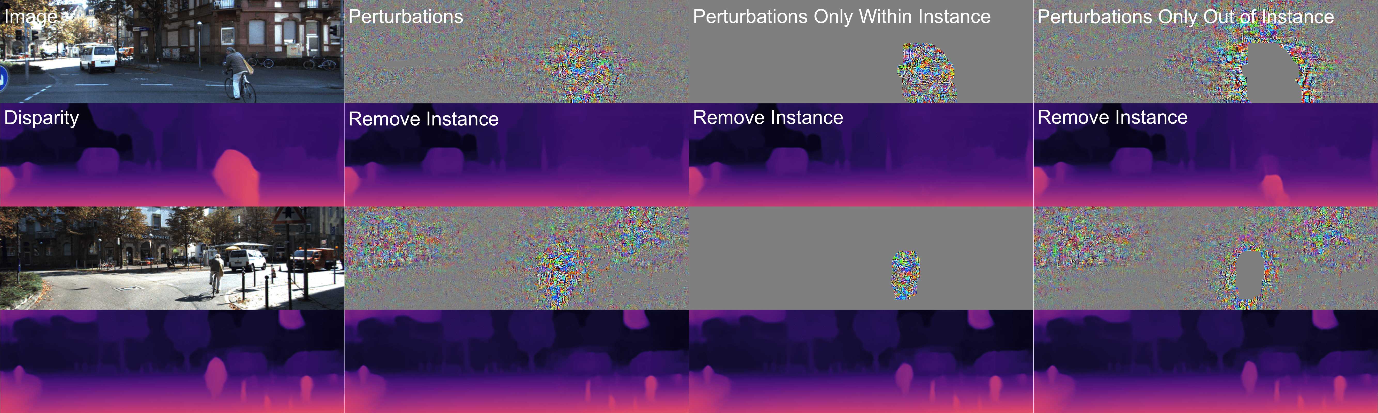
5.2 Instance Conditioned Removing
We now consider the case where instance labels are available for removing a specific instance (e.g. car, pedestrian) from the scene. By examining this scenario, we hope to shed light on the possibility that a depth prediction network can “miss” a human or car, which may cause incorrect rendering in augmented reality or an accident in the autonomous navigation scenario.
Similar to Sec. 5.1, we assume a binary mask , but in this case, of specific instance(s) in the scene, e.g. all pixels belonging to a specific pedestrian are marked with 1 and 0 otherwise. To obtain , we first remove the depth values in belonging to by multiplying by . Then, we use the depth values on the contour of to linearly interpolate the depth in the missing region:
| (5) |
where . Indeed, this scenario is possible. Fig. 8 shows examples of pedestrian and biker removal in the driving scenario where perturbations completely remove the targeted instance. With this attack, the road ahead becomes clear, which makes the agent susceptible to causing an accident.
Even though perturbations are concentrated on the targeted instance region, non-zero perturbations can be observed in the surrounding regions. While the target effect is localized (e.g., make a pedestrian disappear), the perturbation is non-local, implying that the network exploits non-local context, which presents a vulnerability to attacks against a target instance by perturbing other parts of the image. To validate this claim, in the next section, we study perturbations with spatial constraints (either within or outside of the mask) to restrict the information that the adversary can attack.
5.3 Instance Conditioned Removing with Spatial Constraints on the Perturbations
Motivated by our results in Sec. 5.2, we extend the instance conditioned removal task to more constrained scenarios where the perturbations have to either exist (i) completely within the target instance mask or (ii) completely outside of it.
For perturbations within the targeted instance mask , we constrain to satisfy and . When constrained within , perturbations can only remove some instances successfully (e.g. biker is completely removed in row two, column three of Fig. 8). In other cases, the perturbations can only remove the outer part of the instance, leaving parts of the instance in the scene (row four). This shows that depth prediction networks leverage global context; without attacking the contextual information located outside of (e.g. without perturbing the entire image as in column two of Fig. 8), it is not always possible to completely remove the target instance.
Second, we want to answer the question posed in Sec. 1. Can perturbations remove an object by attacking anywhere (e.g. a billboard), but the object (e.g. a car)? In this more challenging case, the perturbations are constrained to be outside of the instance mask: and . Column four of Fig. 8 shows that even though there are no “direct attacks on the object” (perturbations in the masked region), the perturbations can still remove parts of the target instance. While some of the target instance still remains, our experiment demonstrates that depth prediction networks are indeed susceptible to attacks against a target instance that does not require perturbing the instance at all.


5.4 Instance Conditioned Translation
In this case study, we examine perturbations for moving an instance (e.g. vehicle, pedestrian) horizontally or vertically in the image space. As Sec. 5.2 and 5.3 have demonstrated the ability to remove localized objects from the scene, we now show that it is possible for perturbations to move such objects to different locations in the scene (removing the instance and creating it elsewhere) while keeping the rest of the scene unchanged.
Fig. 9-(a) shows that perturbations can fool a network to move the target instance by across the image in the left and right directions. When moved left, the biker (left column) is now in front our vehicle. When moved right, the truck (right column) is in the wrong lane and looks to be on-coming traffic. Moreover, Fig. 9-(b) shows that perturbations can move select instances by in the upward direction, creating the illusion that there are “flying cars” in the scene.


6 Transferability Across Different Models
Transferability is important for black-box scenarios, a practical setting where the attacker does not have access to the target model or its training data. To examine transferability, we test our perturbations crafted for Monodepth2 [16] to fool its predecessor Monodepth [15] (both use 2D convolutions and similar loss functions) in Monodepth2Monodepth, and vice versa in MonodepthMonodepth2, for the scene scaling task. (Sec. 4.1). To consider networks with different architectures and loss functions, we also test perturbations crafted for Monodepth and Monodepth2 on PackNet [18] (3D convolutions) in Fig. 10.
To this end, we also optimized perturbations for Monodepth and PackNet to scale the entire scene. Overall, the perturbations optimized for one model does not transfer to another. Fig. 10 shows that perturbations crafted for networks with different architectures do not transfer. When comparing models with similar architectures and loss, interestingly, transferability decays with increasing norm (Fig. 11), which may be due to perturbations overfitting to the model. We summed the perturbations for Monodepth and Monodepth2 (“Sum” in Fig. 11) and found that their summation can affect both models with reduced effects as the upper norm increases. For , the potency is nearly unaffected, meaning, for small norms, their summation can attack both models equally well. Lastly, by optimizing for both models (“Both” in Fig. 11), the same perturbation can fool both as if it was optimized for the models individually, with performance indistinguishable from MonodepthMonodepth and Monodepth2Monodepth2 across all norms. This shows that both models share a space that is vulnerable to adversarial attacks. Hence, crafting perturbations for an array of potential models may be an avenue towards achieving absolute transferability across models.
7 Conclusion
Depth prediction networks are indeed vulnerable to adversarial perturbations. Not only can such perturbations alter the perception of the scene, but can also affect specific instances, making the network behave unpredictably, which can be catastrophic in applications that involve interaction with physical space. These perturbations also shed light on the network’s dependency on non-local context for local predictions, making non-local targeted attacks possible. Despite these vulnerabilities, targeted attacks do not transfer and cannot be crafted in real time, so we are safe for now. Yet, the fact that they exist suggests that there is room to improve the representation learned. We hope that our findings on the network’s biases, the effect of context, and robustness of the perturbations can help design more secure and interpretable models that are not susceptible to such attacks.
Broader Impact
Adversarial perturbations highlight limitations and failure modes of deep networks. They have captured the collective imagination by conjuring scenarios where AI goes awry at the tune of imperceptible changes. Some popular media and press has gone insofar as suggesting them as proof that AI cannot be trusted.
While monocular depth prediction networks are indeed vulnerable to these attacks, we want to assure the reader that these perturbations cannot cause harm outside of the academic setting. As mentioned in Sec. 3.1, optimizing for these perturbations is computationally expensive and hence it is infeasible to craft these perturbations in real time. Additionally, they also do not transfer; so, we see little negative implications for real-world applications. However, the fact that they exist implies that there is room for improvement in the way that we learn representations for depth prediction.
Hence, we see the existence of adversaries as an opportunity. Studying their effects on deep networks is also the first step to render a system robust to such a vulnerability. The broader impact of our work is to understand the corner cases and failure modes in order to develop more robust representations. This, in turn, will improve interpretability (or, rather, reduce nonsensical behavior). In the fullness of time, we expect this research to pay a small contribution to benefit transportation safety.
Acknowledgements
This work was supported by ONR N00014-19-1-2229 and ARO W911NF-17-1-0304.
References
- Alhaija et al., [2018] Alhaija, H., Mustikovela, S., Mescheder, L., Geiger, A., and Rother, C. (2018). Augmented reality meets computer vision: Efficient data generation for urban driving scenes. International Journal of Computer Vision (IJCV).
- Casser et al., [2019] Casser, V., Pirk, S., Mahjourian, R., and Angelova, A. (2019). Depth prediction without the sensors: Leveraging structure for unsupervised learning from monocular videos. In Proceedings of the AAAI Conference on Artificial Intelligence, volume 33, pages 8001–8008.
- Chen et al., [2016] Chen, W., Fu, Z., Yang, D., and Deng, J. (2016). Single-image depth perception in the wild. In Advances in Neural Information Processing Systems, pages 730–738.
- Cordts et al., [2016] Cordts, M., Omran, M., Ramos, S., Rehfeld, T., Enzweiler, M., Benenson, R., Franke, U., Roth, S., and Schiele, B. (2016). The cityscapes dataset for semantic urban scene understanding. In Proc. of the IEEE Conference on Computer Vision and Pattern Recognition (CVPR).
- Damasio et al., [1982] Damasio, A. R., Damasio, H., and Van Hoesen, G. W. (1982). Prosopagnosia: anatomic basis and behavioral mechanisms. Neurology, 32(4):331–331.
- Deng et al., [2009] Deng, J., Dong, W., Socher, R., Li, L.-J., Li, K., and Fei-Fei, L. (2009). Imagenet: A large-scale hierarchical image database. In 2009 IEEE conference on computer vision and pattern recognition, pages 248–255. Ieee.
- Dijk and Croon, [2019] Dijk, T. v. and Croon, G. d. (2019). How do neural networks see depth in single images? In Proceedings of the IEEE International Conference on Computer Vision, pages 2183–2191.
- Eigen and Fergus, [2015] Eigen, D. and Fergus, R. (2015). Predicting depth, surface normals and semantic labels with a common multi-scale convolutional architecture. In Proceedings of the IEEE International Conference on Computer Vision, pages 2650–2658.
- Eigen et al., [2014] Eigen, D., Puhrsch, C., and Fergus, R. (2014). Depth map prediction from a single image using a multi-scale deep network. In Advances in neural information processing systems, pages 2366–2374.
- Eykholt et al., [2018] Eykholt, K., Evtimov, I., Fernandes, E., Li, B., Rahmati, A., Xiao, C., Prakash, A., Kohno, T., and Song, D. (2018). Robust physical-world attacks on deep learning visual classification. In Proceedings of the IEEE Conference on Computer Vision and Pattern Recognition, pages 1625–1634.
- Fei et al., [2018] Fei, X., Wong, A., and Soatto, S. (2018). Geo-supervised visual depth prediction. arXiv preprint arXiv:1807.11130.
- Fu et al., [2018] Fu, H., Gong, M., Wang, C., Batmanghelich, K., and Tao, D. (2018). Deep ordinal regression network for monocular depth estimation. In Proceedings of the IEEE Conference on Computer Vision and Pattern Recognition, pages 2002–2011.
- Garg et al., [2016] Garg, R., BG, V. K., Carneiro, G., and Reid, I. (2016). Unsupervised cnn for single view depth estimation: Geometry to the rescue. In European Conference on Computer Vision, pages 740–756. Springer.
- Geiger et al., [2012] Geiger, A., Lenz, P., and Urtasun, R. (2012). Are we ready for autonomous driving? the kitti vision benchmark suite. In 2012 IEEE Conference on Computer Vision and Pattern Recognition, pages 3354–3361. IEEE.
- Godard et al., [2017] Godard, C., Mac Aodha, O., and Brostow, G. J. (2017). Unsupervised monocular depth estimation with left-right consistency. In Proceedings of the IEEE Conference on Computer Vision and Pattern Recognition, pages 270–279.
- Godard et al., [2019] Godard, C., Mac Aodha, O., Firman, M., and Brostow, G. J. (2019). Digging into self-supervised monocular depth estimation. In Proceedings of the IEEE International Conference on Computer Vision, pages 3828–3838.
- Goodfellow et al., [2014] Goodfellow, I. J., Shlens, J., and Szegedy, C. (2014). Explaining and harnessing adversarial examples. arXiv preprint arXiv:1412.6572.
- Guizilini et al., [2020] Guizilini, V., Ambrus, R., Pillai, S., Raventos, A., and Gaidon, A. (2020). 3d packing for self-supervised monocular depth estimation. In Proceedings of the IEEE/CVF Conference on Computer Vision and Pattern Recognition, pages 2485–2494.
- Hendrik Metzen et al., [2017] Hendrik Metzen, J., Chaithanya Kumar, M., Brox, T., and Fischer, V. (2017). Universal adversarial perturbations against semantic image segmentation. In Proceedings of the IEEE International Conference on Computer Vision, pages 2755–2764.
- Hu et al., [2019] Hu, J., Zhang, Y., and Okatani, T. (2019). Visualization of convolutional neural networks for monocular depth estimation. In Proceedings of the IEEE International Conference on Computer Vision, pages 3869–3878.
- Ilyas et al., [2019] Ilyas, A., Santurkar, S., Tsipras, D., Engstrom, L., Tran, B., and Madry, A. (2019). Adversarial examples are not bugs, they are features. In Advances in Neural Information Processing Systems, pages 125–136.
- Kingma and Ba, [2014] Kingma, D. P. and Ba, J. (2014). Adam: A method for stochastic optimization. arXiv preprint arXiv:1412.6980.
- Laidlaw and Feizi, [2019] Laidlaw, C. and Feizi, S. (2019). Functional adversarial attacks. In Advances in Neural Information Processing Systems, pages 10408–10418.
- Laina et al., [2016] Laina, I., Rupprecht, C., Belagiannis, V., Tombari, F., and Navab, N. (2016). Deeper depth prediction with fully convolutional residual networks. In 3D Vision (3DV), 2016 Fourth International Conference on, pages 239–248. IEEE.
- Liu et al., [2015] Liu, F., Shen, C., and Lin, G. (2015). Deep convolutional neural fields for depth estimation from a single image. In Proceedings of the IEEE Conference on Computer Vision and Pattern Recognition, pages 5162–5170.
- Liu et al., [2016] Liu, F., Shen, C., Lin, G., and Reid, I. (2016). Learning depth from single monocular images using deep convolutional neural fields. IEEE transactions on pattern analysis and machine intelligence, 38(10):2024–2039.
- Luo et al., [2018] Luo, C., Yang, Z., Wang, P., Wang, Y., Xu, W., Nevatia, R., and Yuille, A. (2018). Every pixel counts++: Joint learning of geometry and motion with 3d holistic understanding. arXiv preprint arXiv:1810.06125.
- Mahjourian et al., [2018] Mahjourian, R., Wicke, M., and Angelova, A. (2018). Unsupervised learning of depth and ego-motion from monocular video using 3d geometric constraints. In Proceedings of the IEEE Conference on Computer Vision and Pattern Recognition, pages 5667–5675.
- Moosavi-Dezfooli et al., [2017] Moosavi-Dezfooli, S.-M., Fawzi, A., Fawzi, O., and Frossard, P. (2017). Universal adversarial perturbations. In Proceedings of the IEEE conference on computer vision and pattern recognition, pages 1765–1773.
- Moosavi-Dezfooli et al., [2016] Moosavi-Dezfooli, S.-M., Fawzi, A., and Frossard, P. (2016). Deepfool: a simple and accurate method to fool deep neural networks. In Proceedings of the IEEE conference on computer vision and pattern recognition, pages 2574–2582.
- Mopuri et al., [2018] Mopuri, K. R., Ganeshan, A., and Babu, R. V. (2018). Generalizable data-free objective for crafting universal adversarial perturbations. IEEE transactions on pattern analysis and machine intelligence, 41(10):2452–2465.
- Najafi et al., [2019] Najafi, A., Maeda, S.-i., Koyama, M., and Miyato, T. (2019). Robustness to adversarial perturbations in learning from incomplete data. In Advances in Neural Information Processing Systems, pages 5542–5552.
- Naseer et al., [2019] Naseer, M. M., Khan, S. H., Khan, M. H., Khan, F. S., and Porikli, F. (2019). Cross-domain transferability of adversarial perturbations. In Advances in Neural Information Processing Systems, pages 12885–12895.
- Peck et al., [2017] Peck, J., Roels, J., Goossens, B., and Saeys, Y. (2017). Lower bounds on the robustness to adversarial perturbations. In Advances in Neural Information Processing Systems, pages 804–813.
- Pillai et al., [2019] Pillai, S., Ambruş, R., and Gaidon, A. (2019). Superdepth: Self-supervised, super-resolved monocular depth estimation. In 2019 International Conference on Robotics and Automation (ICRA), pages 9250–9256. IEEE.
- Poggi et al., [2018] Poggi, M., Tosi, F., and Mattoccia, S. (2018). Learning monocular depth estimation with unsupervised trinocular assumptions. In 2018 International Conference on 3D Vision (3DV), pages 324–333. IEEE.
- Qin et al., [2019] Qin, C., Martens, J., Gowal, S., Krishnan, D., Dvijotham, K., Fawzi, A., De, S., Stanforth, R., and Kohli, P. (2019). Adversarial robustness through local linearization. In Advances in Neural Information Processing Systems, pages 13824–13833.
- Ranjan et al., [2019] Ranjan, A., Janai, J., Geiger, A., and Black, M. J. (2019). Attacking optical flow. In Proceedings of the IEEE International Conference on Computer Vision, pages 2404–2413.
- Silberman et al., [2012] Silberman, N., Hoiem, D., Kohli, P., and Fergus, R. (2012). Indoor segmentation and support inference from rgbd images. In European conference on computer vision, pages 746–760. Springer.
- Szegedy et al., [2013] Szegedy, C., Zaremba, W., Sutskever, I., Bruna, J., Erhan, D., Goodfellow, I., and Fergus, R. (2013). Intriguing properties of neural networks. arXiv preprint arXiv:1312.6199.
- Tramèr and Boneh, [2019] Tramèr, F. and Boneh, D. (2019). Adversarial training and robustness for multiple perturbations. In Advances in Neural Information Processing Systems, pages 5858–5868.
- Wang et al., [2018] Wang, C., Miguel Buenaposada, J., Zhu, R., and Lucey, S. (2018). Learning depth from monocular videos using direct methods. In Proceedings of the IEEE Conference on Computer Vision and Pattern Recognition, pages 2022–2030.
- Wong et al., [2020] Wong, A., Mundhra, M., and Soatto, S. (2020). Stereopagnosia: Fooling stereo networks with adversarial perturbations. arXiv preprint arXiv:2009.10142.
- Wong and Soatto, [2019] Wong, A. and Soatto, S. (2019). Bilateral cyclic constraint and adaptive regularization for unsupervised monocular depth prediction. In Proceedings of the IEEE Conference on Computer Vision and Pattern Recognition, pages 5644–5653.
- [45] Xie, C., Wang, J., Zhang, Z., Zhou, Y., Xie, L., and Yuille, A. (2017a). Adversarial examples for semantic segmentation and object detection. In Proceedings of the IEEE International Conference on Computer Vision, pages 1369–1378.
- [46] Xie, S., Girshick, R., Dollár, P., Tu, Z., and He, K. (2017b). Aggregated residual transformations for deep neural networks. In Proceedings of the IEEE conference on computer vision and pattern recognition, pages 1492–1500.
- Yang et al., [2018] Yang, N., Wang, R., Stückler, J., and Cremers, D. (2018). Deep virtual stereo odometry: Leveraging deep depth prediction for monocular direct sparse odometry. In European Conference on Computer Vision, pages 835–852. Springer.
- Yin et al., [2019] Yin, W., Liu, Y., Shen, C., and Yan, Y. (2019). Enforcing geometric constraints of virtual normal for depth prediction. In Proceedings of the IEEE International Conference on Computer Vision, pages 5684–5693.
- Yin and Shi, [2018] Yin, Z. and Shi, J. (2018). Geonet: Unsupervised learning of dense depth, optical flow and camera pose. In Proceedings of the IEEE Conference on Computer Vision and Pattern Recognition, pages 1983–1992.
- Zhou et al., [2017] Zhou, T., Brown, M., Snavely, N., and Lowe, D. G. (2017). Unsupervised learning of depth and ego-motion from video. In CVPR, volume 2, page 7.
- Zoran et al., [2015] Zoran, D., Isola, P., Krishnan, D., and Freeman, W. T. (2015). Learning ordinal relationships for mid-level vision. In Proceedings of the IEEE International Conference on Computer Vision, pages 388–396.
Supplementary Materials
Appendix A Summary of Contents
In Sec. B, the robustness of perturbations against defenses is discussed. Additional implementation details that we could not fit into main text due to space constraints are given in Sec. C. We verify our claim that targeted adversarial perturbations are visually imperceptible in Sec. D. More experimental results on changing the scale of the scene are provided in Sec. E. In Sec. F, existence of the successful adversarial attacks for indoor scenes (NYU-V2) is shown for state-of-the-art indoor monocular depth prediction model. In Sec. G, we examine how predictions behave when linear operations are applied to perturbations (sum of two perturbations and linear scaling of a perturbation). Failure cases for the perturbations are analyzed in Sec. H. Finally, in Sec. I, more qualitative and quantitative results are provided for the experiments whose compressed versions are presented in the main text.
Appendix B Robustness of the Targeted Attacks Against Defense Mechanisms
In the main text, we have shown that depth prediction networks are prone to adversarial attacks. In this section, we will examine the robustness of the perturbations against common defense mechanisms: (i) Gaussian blurring and (ii) adversarial training.
B.1 Defense through Gaussian Blurring
In Fig. 12, we show the effect of Gaussian blurring as a simple defense mechanism on our targeted attacks by blurring the image with additive perturbations. Even though Gaussian blur does reduce the effectiveness of the perturbations (increased ARE over all scales), the resulting scene is still only away from a target depth that is 10% closer or farther than the original predictions for . This is the performance that the method achieves for the case of without blurring. In other words, the effect of the blurring can be suppressed simply by increasing the upper norm of the noise by for scaling the scene by .


B.2 Defense through Adversarial Training
To examine the robustness of adversarial perturbations to adversarial training, we crafted adversarial perturbations for scaling the scene by a factor of where for the KITTI Eigen split [8] (consisting of 22600 stereo pairs). We trained Monodepth2 [16] by minimizing the normalized discrepancy between the predicted depth of a perturbed image () and its prediction for the original image ().
| (6) |
Fig. 13 shows the effect of the perturbations on Monodepth2 after adversarial training. While training does reduce the influence of adversarial perturbations on the scene scaling task, it does not make the network invariant to the adversarial perturbations. With perturbations of , the predicted scene is from the target scene that is closer than or farther from the original and from the target scene that is closer or farther. For , perturbations can still fool the network to be predict a target scene scaled by with absolute relative error and error for fooling the network to predict a target scene that is scaled by .
To compare the two defense mechanisms, we refer to Fig. 14. For smaller norms, e.g. , we observe a similar performance in using Gaussian blur (Sec. B.1) and adversarial training as defenses against adversarial perturbations; whereas, adversarial training is clearly better for larger . This may be due to Gaussian blur’s ability to destroy the perturbation for small norms and, hence, able to mitigate the effect of the perturbations. However, for larger norms, the blurring does not corrupt the perturbations enough and therefore does not reduce the effect of perturbations by as much.


Appendix C Additional Implementation Details for Outdoor Scenario
In this section, we provide the additional implementation details for crafting adversarial perturbations for Monodepth [15] and Monodepth2 [16] on the KITTI dataset (outdoor driving scenario) as discussed in the main text.
C.1 Hyper-parameters
| Upper Norm | ||||
|---|---|---|---|---|
| Monodepth | ||||
| Monodepth2 |
Regarding hyper-parameters for crafting adversarial perturbations: We search the learning rate for each noise norm from the set . We report the best performing ones in Table 1. Regarding our choice for the number of steps to run, we experimented with 200, 400, 500, 800, and 1000 steps and found little difference in performance measured by ARE between 500 steps, and 800 and 1000 steps. While an increased number of steps will obtain slight performance improvements, conscious of the time complexity, we chose 500 for our experiments.
Regarding hyper-parameters for adversarial training: As a defense against adversarial perturbations, we optimized Eqn. 6 for Monodepth2 using Adam [22] with and . We used a batch size of 4 and starting learning rate of . We decreased the learning rate to after 10 epochs and to after 20 epochs and after 30 epochs for a total of 40 epochs. Training takes approximately 4 hours using an Nvidia GeForce GTX 1080 GPU.
C.2 Monodepth, Monodepth2, and PackNet
We study the effects of adversarial perturbations on the state-of-the-art monocular depth prediction method, PackNet [18], Monodepth2 [16] and its predecessor Monodepth [15]. Monodepth2 and Monodepth models utilize similar 2D convolutional network architectures and are also trained with similar loss functions. PackNet is built on 3D convolutions and uses a different loss function than Monodepth models. In this section, we provide details on the three methods.
Regarding Monodepth: Monodepth uses a ResNet50 encoder architecture as its backbone and a standard decoder with skip connections. Monodepth predicts both left and right disparities from a single image (assuming it is the left image of a stereo-pair) and uses image reconstruction as supervision. Additionally, it is trained with a standard local smoothness term weighted by image gradients and a left-right disparity consistency term as its regularizers.
Regarding Monodepth2: Monodepth2, unlike Monodepth, uses ResNet18 encoder (pretrained on ImageNet) as its backbone network architecture. Rather than simply minimizing an image reconstruction loss, Monodepth2 leverages a heuristic to discount occluded pixels and also uses a criterion to discount static frames. Similar to Monodepth, Monodepth2 also minimizes a local smoothness regularizer weighted by image gradients.
Regarding PackNet: PackNet uses 3D convolutions. While the general architecture is still of the encoder-decoder form, they use “packing” and “unpacking” to convert 2D features into 3D features. PackNet and the Monodepth methods all leverage structure from motion, but PackNet also uses velocity at every time step as a prior to obtain metric depth.
Appendix D Imperceptibility
While we have provided the norm (from to ) and norm (ranging from 0.0124 to 0.0348, depending on the target scene) of the perturbations in the main text, it is difficult to quantify how “visually imperceptible” these perturbations really are. The real test is whether a human can spot the difference between the original and perturbed image. Hence, we conducted a study with 28 people where we ask if two images (the original image paired with itself or its associated perturbed image with the highest norm, ) are the same. The perturbation types were randomly chosen from scaling , horizontal, or vertical flipping. Of the 40 random pairs (20 perturbed), users identified only 1 perturbed image on average, which verifies our claim on the imperceptibility of the perturbations.
Appendix E Scaling with Larger Factors
In Sec. 4.1 and Fig. 2-(a, b) of the main text, we showed that it is possible, even for small norms such as to scale the scene to be or closer or farther with small error. In this section, we demonstrate that it is possible to scale the scene by larger amounts (up to closer or farther). Fig. 15 shows that with , it is only able to scale the up to with reasonable error; whereas perturbations with can achieve this up to closer or farther. However, using larger norms ( and ), one can scale the scene up to with small errors (less than ARE for and ARE for ).
To see how far we can push for each upper norm, Fig. 20 shows various scales that each upper norm is capable of achieving. We note that , is still able to obtain less than ARE when scaling the scene by ; however, standard deviation starts to grow larger as the scaling increases.


Appendix F Adversarial Attacks for Indoor Scenes


To show the applicability of the adversarial method on indoor scenes, we examine the adversarial perturbations for Kinect Dataset NYU Depth V2 (NYU-V2) [39]. We tested the effectiveness of adversarial perturbations on Virtual Normal Loss (VNL) [48] which is the state-of-the-art monocular depth prediction method for NYU-V2, trained in the supervised setting.
F.1 Implementation Details
NYU-V2 consists of 1449 RGBD images gathered from a wide range of buildings, comprising 464 different indoor scenes across 26 scene classes. The images were hand-selected from 435,103 video frames, to ensure diversity. 1449 labeled samples are split into 795 training and 654 test images.
In the method proposed by [48], a 3D point cloud is reconstructed from the estimated depth map. Then, three non-colinear points are randomly sampled with large distances to form a virtual plane. The deviation between ground truth and prediction for the direction of the normal vector corresponding to the plane is penalized. The pre-trained ResNeXt-101 [46] model on ImageNet [6] is used as the backbone architecture. During training, images are cropped to the size 384384 for NYU-V2. We use the same image resolution for our experiments. The training set is randomly sampled from 29K images of the raw unlabeled training set.
The time it takes to forward an image with this method is seconds ( times more than Monodepth2). Due to computational limitations, we choose the first images out of images of the test split for our experiments. We run SGD for steps. The learning rate is kept at for the entire optimization.
F.2 Scaling and Symmetrically Flipping the Scene
In Fig. 16, we compare the performance for different target depth maps: scaling the scene by , horizontal and vertical flipping. Unlike outdoor case (KITTI), in the indoor (NYU-V2) horizontal flipping is a harder task than vertical flipping. Achieving a vertically flipped scene was expected to be simpler as layouts of indoor scenes are more diverse. Hence, the depth network does not overfit to a particular layout type e.g. the one in which there are large depth values only at the top of the image. Horizontal flipping being relatively harder for indoor scenes can be explained by the large divergence between the depth distributions of the original predictions and the target depths. The reason is that for the indoor scenes, most scenes are not symmetric in the horizontal direction, unlike the outdoor driving scenario where the left and right parts of the scene from the ego-view are usually symmetric.
Since [48] normalizes images with the deviation of the dataset which approximately scales the image by , it also effectively scales the noise with the same deviation. But, since the relative norm is still the same, we use the same norm values when plotting the ARE in Fig. 16.
In Fig. 17, we present qualitative results for NYU-V2 for . Small, white borders around RGB images exist in the raw dataset. For all the tasks, including vertical flip, adversarial perturbations manage to fool the model to predict the target depth with small errors. For horizontally flipped target depth (a), predictions have more artifacts than vertical flipped depth (b) and scaled depths (c,d).
Appendix G Linear Operations


To better understand how predictions of the depth network changes within a ball of small radius, we examine the effect of linear operations on perturbations. Specifically, we visualize the predictions for the scaled perturbations and for the perturbations which we get after summing two perturbations calculated for two different target depth maps.
In Fig. 18, we take the perturbation , which we calculated to horizontally flip the prediction for the given image, and we visualize the prediction of the network for where . As can be seen, between and , the scene is smoothly flipped. This implies that the adversarial perturbations can be used to control the depth prediction in a disentangled way. In other words, one causal factor (e.g. horizontal orientation) of the prediction can be independently controlled by tweaking only, keeping everything else the same.
As observed before, noise is small for the white regions. See the third column, where there is a gray rectangle in the noise corresponding to the white region of the truck. We speculate the reason behind this phenomenon as the white color being on the border of the support of RGB images. But, the noise is still large for black regions which are at the other extreme of the support (see perturbations corresponding to black vehicles). So, we left further understanding of this phenomenon as future work.
In Fig. 19, we take and which are optimized to scale the scene to 10% closer and 10% farther. Then, visualize the summed perturbation, and the prediction for . As can be seen, two noises cancel each other: . Furthermore, the prediction for the image perturbed with the summed noise is close to the original prediction: . This shows that two perturbations with inverse functionalities can neutralize their effects when applied together.
Appendix H Failure Cases


Fig. 20 shows the absolute relative error (ARE) with respect to the target scaling factor for each upper norm. As we can see, for smaller norms of and , the perturbations are limited to scaling the scene by and , respectively. Scaling factors higher than such increases the ARE by for every 5% increase in scaling factor, signaling the limit for these norms. For larger norms of and , the perturbations can afford to scale the scene by a much larger factor. For , perturbations can scale the scene by as much as closer and farther less than error. Whereas, for , perturbations can scale the scene up to with less than ARE. However, while large scaling still as a low ARE, the standard deviation for larger norms increases drastically showing that it can no longer consistently scale the scene.
While for smaller scales (e.g. , ) the ARE and amount of noise required is approximately the same (see Sec. 4.1, main text), suggesting similar difficulty levels. As we plot the errors for larger scales in Fig. 20, scaling the scene farther generally yields lower error than scaling the scene closer.
Appendix I Additional Results on Outdoor Scenarios
In this section, we show (i) side by side visualization of the perturbations required to scale the scene, (ii) additional visualizations of perturbations to horizontally and vertically flip the scene, (iii) quantitative results on targeted attacks to semantic categories and (iv) qualitative results on targeted attacks to instances.
I.1 Scaling the Scene

Here, we show qualitative results for the task of scaling the scene (Sec. 4.1, main text) by a factor of where . As seen in Fig. 22, the perturbations are successful in fooling state-of-the-art monocular depth prediction method, Monodepth2 [16], into predicting the scene 5% or 10% closer and also 5% or 10% farther. Additionally, the perturbations are concentrated in similar regions for scaling the scene 5% or 10% closer and for 5% or 10% farther as well. As noted in the main text, the amount of noise required for scaling the scene by are approximately the same, as is the amount for scaling the scene by . This is visible in Fig. 22.
I.2 Symmetrically Flipping the Scene
In Sec. 4.2 and Fig. 3 in the main text, we demonstrated that adversarial perturbation can cause a monocular depth prediction network to predict a horizontally or vertically flipped scene. Here, we show additional qualitative results on the horizontal and vertical flipping tasks in Fig. 23 and Fig. 24. We note that perturbations can cause the network to predict a horizontally flip scene, they have trouble fooling the network to predict a vertically flipped scene. This is unlike our findings in the indoor scenario (Sec. F) as seen in Fig. 17 and 16. Fooling the network to vertically flip the scene is in fact easier than fooling it to horizontally flip the scene. This confirms the biases (roads on bottom, sky on top) that the network learned from the outdoor dataset that are not present in the indoor dataset.


I.3 Category Conditioned Scaling
In Sec. 5.1 and Fig. 5 of the main text, we showed category specific attacks to scale all objects belonging a given category to be a factor of closer or farther where . Here, we provide performance, measured in ARE, of adversarial perturbations crafted for each category. We use the same convention for grouping different classes into categories as the Cityscapes dataset [4], with the exception of the “Human” category, which includes the bicycles that the bikers are riding.
Fig. 25 shows a comparative study between different categories. Not all categories are equally easy to be fooled by the perturbations, some are more robust to adversarial attacks than others. As seen in Fig. 25, each category exhibits a different level of robustness to adversarial noise – “Human” and “Traffic” categories are the hardest to fool, “Construction”, “Vehicle” and “Flat” are more susceptible, and “Sky” and “Nature” are the easiest to attack. Plots are cropped at the maximum error across different categories to enable comparison of difficulty in fooling different categories. We note that attacking localized regions in the scene is considerably harder than attacking the entire scene. Fig. 15 shows that perturbations can attack the entire scene with small errors across various norms while Fig. 25 shows that, even with large norms, there are still errors ( to ARE). We show visualizations for the “Construction”, “Nature”, and “Vehicle” categories in Fig. 26, 27, and 28 respectively.


I.4 Instance Conditioned Targeted Attacks


In Sec. 5.2 and Fig. 6 in the main text, we show that, when given instance segmentation, adversarial perturbations can target specific instances and remove them from the scene and thus causing unforseen consequences. Fig. 29 shows additional examples of removing humans from the scene and Fig. 30 demonstrates that it is possible to remove vehicles from the scene as well. In the rightmost panel of Fig. 29, we show that it is possible to remove some pedestrians from the scene without affecting others. Similarly, in the rightmost panel of Fig. 30, we removed a truck and a car on the right side and left the cars in the center untouched – leaving this as still a plausible highway driving scenario.
In Sec. 5.4 and Fig. 7 in the main text, we show that perturbations can move an instance to another location in the scene (requires removing the instance from its original location and creating it in the new location). In this section, we give more visuals for the perturbations used for moving an instance (e.g. vehicle, pedestrian) horizontally or vertically in the image space while keeping the rest of the scene unchanged.
Fig. 31 shows that perturbations can fool a network to move the target instance by across the image in the left and right directions. Furthermore, Fig. 32 shows that perturbations can move select instances by in the upward direction, creating the illusion that there are “flying vehicles” in the scene. We note that in both cases, the perturbations are concentrated on the instance and the region to which the instance is moved. For example, when moving a vehicle right or left, the corresponding perturbations also move right or left.