Quantum-enhanced interferometry with large heralded photon-number states

We pick 150-fs pulses from a mode-locked Ti:Sapphire laser (Coherent Mira-HP) at a rate of 100 kHz using a Pockels-cell-based pulse picker having a 50 dB extinction ratio. This repetition rate is chosen to accommodate the recovery time of the transition edge sensor detectors. The pump pulses are filtered to $783$ $\pm~2$ nm [full-width at half maximum] using a pair of angle-tuned bandpass filters. We split the pulses into two paths that are matched in length using a translation stage. In each path, we pump a 8 mm long ppKTP waveguide that is phase-matched for type-II parametric down-conversion. At the exit of the waveguide, the pump light is rejected with a longpass filter, and the orthogonally-polarized down-converted modes are separated using a polarizing beam splitter. Each down-converted mode is filtered with a bandpass filter whose bandwidth is chosen to transmit the main feature of the down-converted spectrum but reject its side-lobes. The herald modes ($1566$ $\pm~7$ nm) are coupled into single-mode fibers and sent directly to the detectors. The signal modes ($1567$ $\pm~7$ nm) are coupled into polarization-maintaining single-mode fibers and sent into the interferometer. Details on the coupling efficiency and the spectral indistinguishability of the signal modes are provided in the Supplementary Discussion 2.

The interferometer is a fiber-based variable beam splitter (Newport F-CPL-1550-P-FP). The splitting ratio is adjusted by controlling the distance between two evanescently-coupled fibers using a micrometer, which is analogous to changing the path length difference between two arms of an interferometer. In fact, any variable beam splitter that coherently splits light into two modes can be described by the same transformation as a Mach-Zender-type interferometer Flórez et al. 2018.

During data acquisition, we scan the distance $x$ between the two evanescently-coupled fibers. To display our data as a function of the interferometer phase, we first calculate the transmission coefficient $T(x)$ of the variable beam splitter using the measured $(1,0,1,0)$ and $(0,1,1,0)$ rates:

At low powers, we find that the quantity $T(x)$ typically varies within $[0.02,0.98]$. To obtain the corresponding phase, we correct for the imperfect visibility:

such that $T_{\mathrm{corr}}(x)$ varies between [0,1]. For a single photon injected into a Mach-Zender type interferometer with phase difference $\phi$ between its two arms, one expects $T_{\mathrm{corr}}(x)=[1-\cos{(\phi)}]/2$. Solving for $\phi$, we find:

Our detectors are superconducting transition edge sensor detectors that operate at a temperature of 85 mK inside a dilution refrigerator. Details on their physical operation can be found in Ref. Lita et al. 2008. An electrical trigger signal from the pump laser begins a 6 $\mu s$ time window of data acquisition during which the detector outputs are amplified and recorded with an analogue-to-digital converter. We use a matched-filter technique in real-time to convert each detector’s output trace into a scalar value Figueroa-Feliciano et al. 2000. The scalar value is then converted into a photon number using bins that are set during an initial calibration run prior to data acquisition.

Here we derive the quantum Fisher information of our generalized Holland-Burnett states. We first consider the ideal lossless case. In general, the quantum Fisher information of a pure state $\ket{\Psi(\phi)}$ that depends on some parameter $\phi$ is given by Braunstein and Caves 1994:

where $\ket{\partial_{\phi}\Psi(\phi)}\equiv\partial_{\phi}\ket{\Psi(\phi)}$. In our case, $\ket{\Psi}$ is the two-mode state inside the interferometer (before the phase shift) and $\ket{\Psi(\phi)}=e^{i\hat{c}^{\dagger}\hat{c}\phi}\ket{\Psi}$ is the state after the phase shift $\phi$ is applied in the upper interferometer mode $c$. After some simple algebra, one finds that $\mathcal{Q}$ is independent of $\phi$ and is determined by:

We wish to calculate $\mathcal{Q}$ for the particular probe $\ket{\Psi}=\hat{U}_{\mathrm{BS}}\ket{h_{1},h_{2}}$ where $\hat{U}_{\mathrm{BS}}$ is the balanced beam splitter unitary transformation. The second term in Eq. (S8) is given by:

where in line (S10) we used the fact that $\hat{U}_{\mathrm{BS}}$ is unitary and in line (S11) we transformed mode $c$ to the input modes $a$ and $b$. The first term in equation (S8) is calculated in a similar manner:

Therefore $\mathcal{Q}$ is given by

Eq. (S20) only applies when there are no losses in the system. In the presence of losses, the probe $\ket{\Psi}$ is transformed to a mixed state $\hat{\rho}$. Then, $\mathcal{Q}$ is calculated using

where $\hat{\rho}(\phi)=e^{-i\hat{c}^{\dagger}\hat{c}\phi}\hat{\rho}e^{i\hat{c}^{\dagger}\hat{c}\phi}$ is the probe state after the phase shift $\phi$ and $\hat{\Lambda}[\hat{\rho}(\phi)]$ is a Hermitian operator called the “symmetric logarithmic derivative” defined implicitly via

We notice that by combining Eq. (S22) with Eq. (S21) we obtain an alternative equation for the QFI

By writing $\hat{\rho}$ in its eigenbasis, $\hat{\rho}=\sum_{i}p_{i}\ket{e_{i}}\bra{e_{i}}$ and writing out the derivative $\partial_{\phi}\hat{\rho}(\phi)=ie^{-i\hat{c}^{\dagger}\hat{c}\phi}[\hat{\rho},\hat{c}^{\dagger}\hat{c}]e^{i\hat{c}^{\dagger}\hat{c}\phi}$, it can be shown that $\mathcal{Q}$ is given by Demkowicz-Dobrzański et al. 2015

which is independent of $\phi$. The sum is taken over all terms with a non-vanishing denominator.

In the main text we compare the performance of our probes to the “optimal states” which provide the largest possible quantum Fisher information given some amount of loss Dorner et al. 2009; Demkowicz-Dobrzanski et al. 2009. A general $N$-photon pure state inside the interferometer can be written in the Fock basis as

In the absence of loss, the optimal state is found by optimizing the coefficients $\{\alpha_{n}\}$ to maximize the quantum Fisher information $\mathcal{Q}=4\left[\braket{\Psi|(\hat{c}^{\dagger}\hat{c})^{2}|\Psi}-\braket{\Psi|\hat{c}^{\dagger}\hat{c}|\Psi}^{2}\right]$.

In the presence of loss, $\ket{\Psi}$ turns into a mixture $\hat{\rho}$ which can be written in the following form

where $\ket{\Psi_{j}}$ do not have to be orthogonal. Due to the convexity of quantum Fisher information, $\mathcal{Q}^{\prime}$ of $\hat{\rho}$ is upper bounded by

The bound is attained if the kets $\ket{\Psi_{j}}$ are orthogonal, which is the case for e.g. N00N states or if photon losses are present in only one interferometer mode.

Applying Eq. (S27) to Eq. (S25), we obtain

where $x_{n}=|\alpha_{n}|^{2}$, $B_{lm}^{n}\equiv\binom{n}{l}\binom{N-n}{m}\eta_{s_{1}}^{n}(\eta_{s_{1}}^{-1}-1)^{l}\eta_{s_{2}}^{N-n}(\eta_{s_{2}}^{-1}-1)^{m}$ and $\eta_{s_{1}},\eta_{s_{2}}$ denote the transmittances in the signal modes.

The optimal states are found by numerically maximizing $\mathcal{Q}$ over the probabilities $\{x_{n}\}$. Since $\mathcal{Q}$ is a concave function of $\{x_{n}\}$ Demkowicz-Dobrzanski et al. 2009, any maximum is global. Although $\mathcal{Q}^{\prime}<\mathcal{Q}$ [Eq. (S27)] when losses are present in both modes, the difference between the two quantities is small relative to the difference between the shot-noise limit and the Heisenberg limit Demkowicz-Dobrzanski et al. 2009. Due to this approximation, the optimized $\mathcal{Q}$ is a slight over-estimate of true quantum Fisher information $\mathcal{Q}^{\prime}$ of the optimal states.

Fig. 1(b) in the main text shows $\mathcal{Q}$ of our probes and the optimal state as a function of equal transmissivity in the signal modes $\eta_{s_{1}}=\eta_{s_{2}}=\eta_{s}$ which varied from 0 to 1 in steps of 0.01. The optimal state was calculated in Mathematica by maximizing over coefficients $\{x_{n}\}$ in Eq. (S28), assuming they all sum up to 1 and are real and positive. We computed $\mathcal{Q}$ of our probes in Python using the following method. We started with two copies of the state in Eq. (1) in the main text, inserted a beam splitter in each signal mode, and traced over the reflected port to model signal transmissivities $\eta_{s}$. The two matrices were then combined on the first interferometer beam splitter forming a four mode density matrix, which was then reduced to two modes by projectively measuring the two herald modes. Eigenvalues and eigenvectors were found for the two-mode density matrix inside the interferometer which were then used to calculate $\mathcal{Q}$ via Eq. (S24). To compare the ideal performance of our probes with the optimal state, we exclude the effect of imperfect heralding on the former by using $\eta_{h_{1}}=\eta_{h_{2}}=1$ in the calculation of $\mathcal{Q}$.

From the calculations described above we show that for $\eta_{s}\in(0,0.5\rangle$ the best approximation to the optimal state is given by the probe with $\Delta=8$; for $\eta_{s}\in(0.5,0.58\rangle$ by the probe with $\Delta=6$; for $\eta_{s}\in(0.58,0.66\rangle$ by the probe with $\Delta=4$; for $\eta_{s}\in(0.66,0.69\rangle$ by the probe with $\Delta=2$; and for $\eta_{s}>0.69$ by the probe with $\Delta=0$, as shown by the colored line in Fig. 1(b).

Here we describe the model $\tilde{\mathrm{pr}}(s_{1},s_{2},h_{1},h_{2},\phi)$ used to fit the experimentally measured rates. We model optical loss by placing fictitious beam splitters (see Fig. S5) and tracing over the reflected modes. For now, we assume $\eta_{d_{1}}=\eta_{d_{2}}=1$. We will treat the effect of these detection losses at the end.

The sources produce two-mode squeezed vacuum states:

where $i=1,2$ represent sources 1 and 2, respectively. The joint photon-number distribution of this two-mode squeezed vacuum state after the losses is given by:

The intuition for the expression above is as follows. Imagine that there are two detectors after the fictitious beam splitters that give the detection outcome $(x,y)$. The source must have produced at least $\max{(x,y)}$ photon pairs and perhaps some photons were lost (i.e. reflected at the beam splitters). The probability to produce $n$ pairs of photons is $(1-\lambda_{i})^{2}\lambda^{2n}_{i}$. Having produced $n$ pairs, the probability to reflect $n-x$ [$n-y$] photons and transmit $x$ [$y$] photons in the herald [signal] mode is ${n\choose x}\eta_{h_{i}}^{x}(1-\eta_{h_{i}})^{n-x}$ [${n\choose y}\eta_{s_{i}}^{y}(1-\eta_{s_{i}})^{n-y}$]. In principle, $n$ can range up to $\infty$, but in practice it suffices to truncate this sum at some value where $(1-\lambda_{i})^{2}\lambda^{2n}_{i}$ becomes small. In our numerics, we truncate the sum at $n=50$.

If we obtain the herald outcome $(h_{1},h_{2})$, then the (unnormalized) state that is injected into the interferometer is given by:

Losses occurring inside the interferometer can be absorbed into $\eta_{s}$ or $\eta_{d}$ if they are equal in both interferometer modes, which was approximately the case in our experiment. Thus, the interferometer transformation can be described by a unitary operator $\hat{U}(\phi)$ which depends on the phase difference $\phi$ between both arms. The probability that we wish to calculate is given by:

Knowing that there are a total of $s_{1}+s_{2}$ photons before the interferometer, we can constrain $n=s_{1}+s_{2}-m$ and truncate the sum at $s_{1}+s_{2}$ in Eq. (S31). Thus, we obtain:

The matrix element $\left|\braket{s_{1},s_{2}|\hat{U}(\phi)|m,s_{1}+s_{2}-m}\right|^{2}$ is derived in Ref. Leonhardt 2010 and is given by:

Alternatively, the matrix element can also be evaluated using Kravchuk polynomials Stobińska et al. 2019.

The model for temporally distinguishable photons follows the same approach as above. While the derivation below focuses on temporal distinguishability, the same equations are valid to describe distinguishability in any other degree of freedom. We adopt a heuristic approach (e.g. as in Ref Birchall et al. 2016) in which the temporal mode of the photons produced in the top source is decomposed into a component completely indistinguishable ($\parallel$) to the temporal mode of the bottom source photons as well as a component completely distinguishable ($\perp$). With this decomposition, Eq. (S31) becomes:

where $\mathcal{M}\in[0,1]$ is a mode overlap parameter characterizing the distinguishability of the photons. For $\mathcal{M}=0$ ($\mathcal{M}=1$), the photons from top and bottom sources are completely distinguishable (indistinguishable). Since our detectors cannot resolve the time difference between $\perp$ and $\parallel$, they convolve the probabilities for the photons to have originated from either temporal mode. This measurement is described by the following incoherent sum of projectors:

Many of the terms in the sum of Eq. (S36) can be eliminated due to constraints on the photon numbers. For example, a total of $m-l$ photons are produced in mode $\perp$ and so $x+y=m-l$. Moreover, $s_{1}+s_{2}=m+n$. After applying these constraints, the final joint probability is given by:

Finally, we can now consider the effect of the losses just before the detectors. These losses can be modelled with a transformation analogous to Eq. (S30). Applying this transformation on Eq. (S33), we obtain:

The same method is used for the distinguishable photons model, i.e. replace $\tilde{\mathrm{pr}}(j,k,h_{1},h_{2},\phi)$ with $\tilde{\mathrm{pr}}^{dist}(j,k,h_{1},h_{2},\phi)$ in Eq. (S38). In our numerics, we truncate the sums in Eq. (S38) to only include the effect of losing a few photons, which is a good approximation given the high efficiency of our number-resolving detectors.

The equations above are evaluated numerically and fitted to the experimentally measured $\mathrm{pr}(s_{1},s_{2},h_{1},h_{2},\phi)$ by varying the fit parameters $\eta_{h_{1}},\eta_{h_{2}},\eta_{s_{1}},\eta_{s_{2}},\eta_{d_{1}},\eta_{d_{2}},\lambda_{1},\lambda_{2}$. Fitting is performed using the Python package lmfit with a least squares method. Note that, for the sake of increasing the speed of the fitting, we used $\mathcal{M}=1$ for all data except for the dashed lines in Fig. 4 of the main text where we used $\mathcal{M}=0$. Thus, the fit parameters generally did not correspond to the measured efficiencies and squeezing parameters (see below). Instead, the fitting procedure converged on larger $\lambda$ values and smaller $\eta$ values to emulate the effect of imperfect interference (i.e. reduced fringe visibility). We tested the full model (i.e. including $\mathcal{M}$) by fitting a subset of rates measured in the high gain regime and found the fit parameters: $\eta_{h_{1}}=0.50$, $\eta_{h_{2}}=0.50$, $\eta_{s_{1}}=0.61$, $\eta_{s_{2}}=0.50$, $\eta_{d_{1}}=0.9$, $\eta_{d_{2}}=0.99$, $\lambda_{1}=0.68$, $\lambda_{2}=0.68$, and $\mathcal{M}=0.73$. These efficiency values are within error to the measured values (see below), and $\mathcal{M}=0.73$ is roughly consistent with the measured $\sim 75\%$ quantum interference visibility of the $(1,1,1,1)$ rate.

We characterize the efficiency of our setup using a Klyshko-like method that is generalized to photon-number-resolving detection Worsley et al. 2009. We set the variable beam splitter to maximize reflection and measure the joint photon-number distribution $\mathrm{pr}_{i}(x,y)$ pumping one source at a time. We fit the measured $\mathrm{pr}_{i}(x,y)$ to $\tilde{\mathrm{pr}}_{i}(x,y)$ [see Eq. (S30)] using three parameters: the PDC gain $\lambda_{i}$ and the total efficiency of the herald mode ($\eta_{h_{i}}$) and the signal mode ($\eta_{s_{i}}$). Note that the latter will also include the detection efficiency $\eta_{d_{i}}$. By repeating the procedure with five different pump powers, we find that $\eta_{s_{1}}\eta_{d_{1}}=56\pm 3\%$ and $\eta_{h_{1}}=47\pm 1\%$ for the first source, and $\eta_{s_{2}}\eta_{d_{2}}=52\pm 4\%$ and $\eta_{h_{2}}=51\pm 1\%$ for the second source.

Here we compare the performance of our measurement strategy, photon counting, to the optimal measurement strategy. In Fig. S6, we plot the classical Fisher information per photon obtained with photon counting for various $N=8$ probes, assuming ideal heralding ($\eta_{h_{1}}=\eta_{h_{2}}=1$) and balanced loss inside the interferometer ($\eta_{s_{1}}=\eta_{s_{2}}=\eta_{s}$). Since this quantity generally depends on $\phi$ when $\eta_{s}<1$, we focus on the region with the largest phase sensitivity, i.e. $\mathrm{max}[\tilde{\mathcal{F}}(\phi)]$ [continuous lines]. In the same plot, we reproduce the quantum Fisher information curves from Fig. 1(b) normalized by the number of detected photons, i.e. $\mathcal{Q}/\eta_{s}N$ [dashed lines]. For $\eta_{s}=1$, the quantum and classical Fisher information are equal which means that photon counting is the optimal measurement strategy, as expected Hofmann 2009. For $\eta_{s}<1$, photon counting is no longer optimal (except for $\Delta=N$) but still provides quantum-enhanced phase sensitivity for $\eta_{s}\gtrsim 0.55$. To the best of our knowledge, the optimal measurement strategy for lossy Holland-Burnett interferometry is not known. We note that homodyne and weak-field homodyne (i.e. combining a signal with local oscillator then performing photon counting) have been shown to be more loss-tolerant than photon counting using Gaussian probes Ono and Hofmann 2010; Oh et al. 2017. However, it remains an open question whether these measurement strategies would be advantageous using our non-Gaussian probes in the presence of loss.

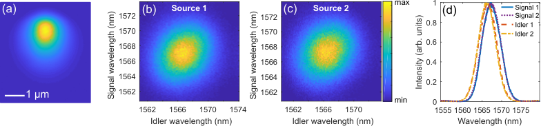
The main imperfections limiting the estimation precision are (i) photon loss and (ii) incomplete interference of the input photons. The main contribution to photon loss ($\sim$50% end-to-end, see Supplementary Method 3) are the inefficiences caused by the spatial overlap between the waveguide mode and the fiber mode. The diffusion process used to produce KTP waveguides leads to non-Gaussian and asymmetric features in the waveguide spatial mode [Fig. S7(a)] which limit the fiber coupling efficiency to $\sim$70%. It may be possible to improve the spatial mode of the waveguide by optimizing the diffusion process Padberg et al. 2020 or employing ridge waveguides Volk et al. 2018. The quantum interference visibility ($\sim 75\%$) is mainly limited by spectral mode mismatch between the signal modes as well as the spectral purity of the sources. We show the joint spectral intensities [Fig. S7(b-c)] and marginal spectra [Fig. S7(d)] of the sources measured using a time-of-flight spectrometer (resolution $\pm 0.1$nm). Although the joint spectral intensities appear decorrelated and the signal spectra are well overlapped, we suspect that non-uniform spectral phase (perhaps due to pump chirp or dispersion through optical elements) may have reduced the quantum interference visibility. Moreover, the spectral purity is degraded by uncorrelated background photons ($\sim 5\%$ of detected photons). These background photons are generated in a continuum of spectral modes and likely originate from processes where one photon from a down-converted pair is generated in an unguided waveguide mode Eckstein 2012, in which case their contribution could be reduced by minimizing propagation losses inside the waveguide.

Using the $\Delta=N$ probe, all photons injected into the interferometer originate from one source. As such, imperfections such as spectral purity and mode matching should not affect the performance of the probe. The $\Delta=N$ probe is prepared by considering trials where e.g. $(h_{1},h_{2})=(N,0)$. However, even when $h_{2}=0$, this second source can still inject unwanted light into the interferometer due to losses in the herald modes. This generally degrades the performance of the $\Delta=N$ probe. Here we show that shot-noise limited performance is recovered by blocking one of the sources. In Fig. S8, we plot $\tilde{\mathcal{F}}_{5,0}(\phi)$ for the $\Delta=N=5$ probe calculated without post-selection. We performed the measurement with a single source blocked and with both sources unblockled. In the latter case, we find that $\tilde{\mathcal{F}}_{5,0}(\phi)$ reaches $0.991\pm 0.001$ at its highest point, demonstrating shot-noise limited performance. Ideally, $\tilde{\mathcal{F}}_{5,0}(\phi)$ should be flat with $\phi$. However, experimental imperfections such as imbalanced detector efficiency, detector dark counts ($\sim 1\%$), and imperfect interferometer visibility cause the dips in $\tilde{\mathcal{F}}_{5,0}(0)$ and $\tilde{\mathcal{F}}_{5,0}(\pm\pi)$ where the photons should ideally always exit the interferometer from one port.

Here we provide an analysis on estimating the efficiency and quality of the two-mode vacuum sources required to surpass the shot-noise limit without post-selection. We focus on the $\Delta=6$ [i.e. $(h_{1},h_{2})=(7,1)$] probe as this is the most loss-tolerant $N=8$ probe that can surpass the shot-noise limit in our scheme. For simplicity, we assume equal efficiency $\eta$ in all four modes of the experiment ($\eta=\eta_{h_{1}}=\eta_{h_{2}}=\eta_{s_{1}}=\eta_{s_{2}}$) and equal PDC gain parameters $\lambda$. There are three main experimental parameters to consider: (i) the efficiency $\eta$, (ii) the distinguishability $\mathcal{M}$ of photons between the top and bottom sources, (iii) the PDC gain $\lambda$. Given these parameters, we estimate the sensitivity of the probe by calculating the classical Fisher information $\tilde{\mathcal{F}}_{7,1}(\phi)$ (per detected signal photon). Since this quantity generally depends on $\phi$, we focus on region in phase with the largest possible sensitivity, i.e. $\max[\tilde{\mathcal{F}}_{7,1}(\phi)]$.

We begin by focusing on the effect of the PDC gain $\lambda$ and assume $\mathcal{M}=1$ for now. As shown in Fig. S9(a), a smaller $\lambda$ provides a larger $\mathrm{max}[\tilde{\mathcal{F}}_{7,1}(\phi)]$. This is because lowering $\lambda$ increases the photon-number purity of the heralded probe in the presence of loss in the heralding arms, i.e. it reduces the probability that the herald detectors under-counted the true number of photon pairs produced by the sources. As a reference, we include the perfect heralding case which is shown by the black line. While reducing $\lambda$ minimizes the detrimental effects of imperfect heralding, it also drastically decreases the heralding rate. For example, assuming $\eta=0.5$ and a 100 kHz laser repetition rate, $\lambda=0.75$ would produce a $N=8$ probe roughly once per second whereas $\lambda=0.35$ would produce such a probe only about once per day.

Next we consider the combined effect of imperfect distinguishability and efficiency. In Fig. S9(b) [(c)], we plot $\mathrm{max}[\tilde{\mathcal{F}}_{7,1}(\phi)]$ as a function of $\eta$ and $\mathcal{M}$ for $\lambda=0.75$ [$\lambda=0.35$]. The approximate region achieved in our experiment is shown in yellow. Improvements in both $\eta$ and $\mathcal{M}$ are necessary to unconditionally surpass the shot-noise limit. As a reference point, a distinguishability of $\mathcal{M}\sim 0.85$ was achieved in Ref. Stobińska et al. 2019 using the same type of high-gain PDC sources as used in our experiment. With such a distinguishability, the efficiency would need to be improved to $\sim 80\%$ [$\sim 70\%$] when using $\lambda=0.75$ [$\lambda=0.35$].

References

- Demkowicz-Dobrzański et al. (2015) R. Demkowicz-Dobrzański, M. Jarzyna, and J. Kołodyński, in Progress in Optics, Vol. 60 (Elsevier, 2015) pp. 345–435.
- Caves (1981) C. M. Caves, Phys. Rev. D 23, 1693 (1981).
- Tse et al. (2019) M. Tse et al., Phys. Rev. Lett. 123, 231107 (2019).
- Crespi et al. (2012) A. Crespi, M. Lobino, J. C. Matthews, A. Politi, C. R. Neal, R. Ramponi, R. Osellame, and J. L. O’Brien, App. Phys. Lett. 100, 233704 (2012).
- Wolfgramm et al. (2013) F. Wolfgramm, C. Vitelli, F. A. Beduini, N. Godbout, and M. W. Mitchell, Nat. Photonics 7, 28 (2013).
- Taylor et al. (2013) M. A. Taylor, J. Janousek, V. Daria, J. Knittel, B. Hage, H.-A. Bachor, and W. P. Bowen, Nat. Photon. 7, 229 (2013).
- Taylor and Bowen (2016) M. A. Taylor and W. P. Bowen, Phys. Rep. 615, 1 (2016).
- Cimini et al. (2019) V. Cimini, M. Mellini, G. Rampioni, M. Sbroscia, L. Leoni, M. Barbieri, and I. Gianani, Opt. Express 27, 35245 (2019).
- Bollinger et al. (1996) J. J. Bollinger, W. M. Itano, D. J. Wineland, and D. J. Heinzen, Phys. Rev. A 54, R4649 (1996).
- Mitchell et al. (2004) M. W. Mitchell, J. S. Lundeen, and A. M. Steinberg, Nature 429, 161 (2004).
- Walther et al. (2004) P. Walther, J.-W. Pan, M. Aspelmeyer, R. Ursin, S. Gasparoni, and A. Zeilinger, Nature 429, 158 (2004).
- Nagata et al. (2007) T. Nagata, R. Okamoto, J. L. O’Brien, K. Sasaki, and S. Takeuchi, Science 316, 726 (2007).
- Kim et al. (2009) H. Kim, H. S. Park, and S.-K. Choi, Opt. Express 17, 19720 (2009).
- Afek et al. (2010) I. Afek, O. Ambar, and Y. Silberberg, Science 328, 879 (2010).
- Matthews et al. (2011) J. C. F. Matthews, A. Politi, D. Bonneau, and J. L. O’Brien, Phys. Rev. Lett. 107, 163602 (2011).
- Ulanov et al. (2016) A. E. Ulanov, I. A. Fedorov, D. Sychev, P. Grangier, and A. Lvovsky, Nat. Commun. 7, 11925 (2016).
- Slussarenko et al. (2017) S. Slussarenko, M. M. Weston, H. M. Chrzanowski, L. K. Shalm, V. B. Verma, S. W. Nam, and G. J. Pryde, Nat. Photonics 11, 700 (2017).
- Datta et al. (2011) A. Datta, L. Zhang, N. Thomas-Peter, U. Dorner, B. J. Smith, and I. A. Walmsley, Phys. Rev. A 83, 063836 (2011).
- Dorner et al. (2009) U. Dorner, R. Demkowicz-Dobrzański, B. J. Smith, J. S. Lundeen, W. Wasilewski, K. Banaszek, and I. A. Walmsley, Phys. Rev. Lett. 102, 040403 (2009).
- Kacprowicz et al. (2010) M. Kacprowicz, R. Demkowicz-Dobrzański, W. Wasilewski, K. Banaszek, and I. Walmsley, Nat. Photonics 4, 357 (2010).
- Demkowicz-Dobrzański et al. (2013) R. Demkowicz-Dobrzański, K. Banaszek, and R. Schnabel, Phys. Rev. A 88, 041802 (2013).
- Lang and Caves (2013) M. D. Lang and C. M. Caves, Phys. Rev. Lett. 111, 173601 (2013).
- Yonezawa et al. (2012) H. Yonezawa, D. Nakane, T. A. Wheatley, K. Iwasawa, S. Takeda, H. Arao, K. Ohki, K. Tsumura, D. W. Berry, T. C. Ralph, H. M. Wiseman, E. H. Huntington, and A. Furusawa, Science 337, 1514 (2012).
- Berni et al. (2015) A. A. Berni, T. Gehring, B. M. Nielsen, V. Händchen, M. G. Paris, and U. L. Andersen, Nat. Photon. 9, 577 (2015).
- Holland and Burnett (1993) M. J. Holland and K. Burnett, Phys. Rev. Lett. 71, 1355 (1993).
- Sun et al. (2008) F. Sun, B. Liu, Y. Gong, Y. Huang, Z. Ou, and G. Guo, EPL 82, 24001 (2008).
- Xiang et al. (2011) G.-Y. Xiang, B. L. Higgins, D. Berry, H. M. Wiseman, and G. Pryde, Nat. Photonics 5, 43 (2011).
- Thomas-Peter et al. (2011) N. Thomas-Peter, B. J. Smith, A. Datta, L. Zhang, U. Dorner, and I. A. Walmsley, Phys. Rev. Lett. 107, 113603 (2011).
- Xiang et al. (2013) G. Xiang, H. Hofmann, and G. Pryde, Sci. Rep. 3, 2684 (2013).
- Jin et al. (2016) R.-B. Jin, M. Fujiwara, R. Shimizu, R. J. Collins, G. S. Buller, T. Yamashita, S. Miki, H. Terai, M. Takeoka, and M. Sasaki, Sci. Rep. 6, 36914 (2016).
- Matthews et al. (2016) J. C. Matthews, X.-Q. Zhou, H. Cable, P. J. Shadbolt, D. J. Saunders, G. A. Durkin, G. J. Pryde, and J. L. O’Brien, npj Quantum Inf. 2, 1 (2016).
- Eckstein et al. (2011) A. Eckstein, A. Christ, P. J. Mosley, and C. Silberhorn, Phys. Rev. Lett. 106, 013603 (2011).
- Harder et al. (2016) G. Harder, T. J. Bartley, A. E. Lita, S. W. Nam, T. Gerrits, and C. Silberhorn, Phys. Rev. Lett. 116, 143601 (2016).
- Lita et al. (2008) A. E. Lita, A. J. Miller, and S. W. Nam, Opt. Express 16, 3032 (2008).
- Gao et al. (2010) W.-B. Gao, C.-Y. Lu, X.-C. Yao, P. Xu, O. Gühne, A. Goebel, Y.-A. Chen, C.-Z. Peng, Z.-B. Chen, and J.-W. Pan, Nat. Phys. 6, 331 (2010).
- Wang et al. (2016) X.-L. Wang, L.-K. Chen, W. Li, H.-L. Huang, C. Liu, C. Chen, Y.-H. Luo, Z.-E. Su, D. Wu, Z.-D. Li, H. Lu, Y. Hu, X. Jiang, C.-Z. Peng, L. Li, N.-L. Liu, Y.-A. Chen, C.-Y. Lu, and J.-W. Pan, Phys. Rev. Lett. 117, 210502 (2016).
- Wang et al. (2019) H. Wang, J. Qin, X. Ding, M.-C. Chen, S. Chen, X. You, Y.-M. He, X. Jiang, L. You, Z. Wang, C. Schneider, J. J. Renema, S. Höfling, C.-Y. Lu, and J.-W. Pan, Phys. Rev. Lett. 123, 250503 (2019).
- Stobińska et al. (2019) M. Stobińska, A. Buraczewski, M. Moore, W. Clements, J. J. Renema, S. Nam, T. Gerrits, A. Lita, W. Kolthammer, A. Eckstein, et al., Sci. Adv. 5, eaau9674 (2019).
- Hofmann (2009) H. F. Hofmann, Phys. Rev. A 79, 033822 (2009).
- Zhong et al. (2017) W. Zhong, Y. Huang, X. Wang, and S.-L. Zhu, Phys. Rev. A 95, 052304 (2017).
- Birchall et al. (2016) P. M. Birchall, J. Sabines-Chesterking, J. L. O’Brien, H. Cable, and J. C. Matthews, arXiv preprint arXiv:1603.00686 (2016).
- Resch et al. (2007) K. J. Resch, K. L. Pregnell, R. Prevedel, A. Gilchrist, G. J. Pryde, J. L. O’Brien, and A. G. White, Phys. Rev. Lett. 98, 223601 (2007).
- Humphreys et al. (2015) P. C. Humphreys, B. J. Metcalf, T. Gerrits, T. Hiemstra, A. E. Lita, J. Nunn, S. W. Nam, A. Datta, W. S. Kolthammer, and I. A. Walmsley, New J. Phys. 17, 103044 (2015).
- Pezzé et al. (2007) L. Pezzé, A. Smerzi, G. Khoury, J. F. Hodelin, and D. Bouwmeester, Phys. Rev. Lett. 99, 223602 (2007).
- Daryanoosh et al. (2018) S. Daryanoosh, S. Slussarenko, D. Berry, H. Wiseman, and G. Pryde, Nat. Commun. 9, 2041 (2018).
- Vaidya et al. (2020) V. Vaidya, B. Morrison, L. Helt, R. Shahrokshahi, D. Mahler, M. Collins, K. Tan, J. Lavoie, A. Repingon, M. Menotti, et al., Sci. Adv. 6, eaba9186 (2020).
- Flórez et al. (2018) J. Flórez, N. J. Carlson, C. H. Nacke, L. Giner, and J. S. Lundeen, Rev. Sci. Instrum. 89, 023108 (2018).
- Figueroa-Feliciano et al. (2000) E. Figueroa-Feliciano, B. Cabrera, A. Miller, S. Powell, T. Saab, and A. Walker, Nucl. Instrum. Methods Phys. Res 444, 453 (2000).
- Braunstein and Caves (1994) S. L. Braunstein and C. M. Caves, Phys. Rev. Lett. 72, 3439 (1994).
- Demkowicz-Dobrzanski et al. (2009) R. Demkowicz-Dobrzanski, U. Dorner, B. J. Smith, J. S. Lundeen, W. Wasilewski, K. Banaszek, and I. A. Walmsley, Phys. Rev. A 80, 013825 (2009).
- Leonhardt (2010) U. Leonhardt, Essential quantum optics: from quantum measurements to black holes (Cambridge University Press, 2010).
- Worsley et al. (2009) A. Worsley, H. Coldenstrodt-Ronge, J. Lundeen, P. Mosley, B. Smith, G. Puentes, N. Thomas-Peter, and I. Walmsley, Opt. Express 17, 4397 (2009).
- Ono and Hofmann (2010) T. Ono and H. F. Hofmann, Phys. Rev. A 81, 033819 (2010).
- Oh et al. (2017) C. Oh, S.-Y. Lee, H. Nha, and H. Jeong, Phys. Rev. A 96, 062304 (2017).
- Padberg et al. (2020) L. Padberg, M. Santandrea, M. Rüsing, J. Brockmeier, P. Mackwitz, G. Berth, A. Zrenner, C. Eigner, and C. Silberhorn, Opt. Express 28, 24353 (2020).
- Volk et al. (2018) M. F. Volk, C. E. Rüter, M. Santandrea, C. Eigner, L. Padberg, H. Herrmann, C. Silberhorn, and D. Kip, Opt. Mater. Express 8, 82 (2018).
- Eckstein (2012) A. Eckstein, Mastering quantum light pulses with nonlinear waveguide interactions, Ph.D. thesis, Friedrich-Alexander-Universität Erlangen-Nürnberg (2012).
Supplementary information
Supplementary Note 1: Quantum Fisher information of generalized Holland-Burnett states