On the Loss Landscape of Adversarial Training:
Identifying Challenges and How to Overcome Them

For the simple but special case of logistic regression, i.e., $K=2$, we can write the analytical form of $\mathcal{L}_{\epsilon}(\theta)$. We defer the detailed discussion of this case to Appendix A.1, and here focus on linear multi-class classification, i.e., $K\geq 3$. We parameterize the model by $\mathbf{W}\vcentcolon=\{\mathbf{w}_{i}\}_{i=1}^{K}\in\mathbb{R}^{m\times K}$ and use $f(\mathbf{W})=[\mathbf{w}_{1}^{T}\mathbf{x},\mathbf{w}_{2}^{T}\mathbf{x},...,\mathbf{w}_{K}^{T}\mathbf{x}]$ as the logit function. Therefore, the vanilla loss function is convex as $g(\mathbf{x},\mathbf{W})=\log(1 + \sum_{j \neq y}\exp^{(\w_j - \w_y)^T\x})$. Although $g_{\epsilon}(\mathbf{x},\mathbf{W})$ is also convex, it is no longer smooth everywhere. It is then difficult to write a unified expression of $g_{\epsilon}(\mathbf{x},\mathbf{W})$. So we start with the version space $\mathcal{V}_{\epsilon}$ of $g_{\epsilon}(\mathbf{x},\mathbf{W})$ defined as $\mathcal{V}_{\epsilon}=\left\{\mathbf{W}\bigg\rvert(\mathbf{w}_{i}-\mathbf{w}_{y})\mathbf{x}^{\prime}\leq 0,\forall i\in[K],\mathbf{x}^{\prime}\in\mathcal{S}_{\epsilon}(\mathbf{x})\right\}$.

By definition, $\mathcal{V}_{\epsilon}$ is the smallest convex closed set containing all solutions robust under the adversarial budget $\mathcal{S}_{\epsilon}(\mathbf{x})$. The proposition below states that the version space $\mathcal{V}_{\epsilon}$ shrinks with larger values of $\epsilon$.

The proof of Proposition 1 is very straightforward, we put it in Appendix B.1.

In addition to $\mathcal{V}_{\epsilon}$, we define the set $\mathcal{T}_{\epsilon}$ as $\mathcal{T}_{\epsilon}=\left\{\mathbf{W}\bigg\rvert 0\in\argmin_{\gamma}g_{\epsilon}(\mathbf{x},\gamma\mathbf{W})\right\}$. $\mathcal{T}_{\epsilon}$ is the set of all directions in which the optimal point is the origin; that is, the corresponding models in this direction are all no better than a constant classifier. Although we cannot write the set $\mathcal{T}_{\epsilon}$ in roster notation, we show in the theorem below that $\mathcal{T}_{\epsilon}$ becomes larger as $\epsilon$ increases.

We defer the proof of Theorem 1 to Appendix B.2, where we also provide a lower bound for $\bar{\epsilon}$. Theorem 1 indicates that when the adversarial budget is large enough, the optimal point is the origin. In this case, we will get a constant classifier, and training completely fails.

$\mathcal{L}_{\epsilon}(\mathbf{W})$ is the average of $g_{\epsilon}(\mathbf{x},\mathbf{W})$ over the dataset, so Theorem 1 and Proposition 1 still apply if we replace $g_{\epsilon}$ with $\mathcal{L}_{\epsilon}$ in the definition of $\mathcal{V}_{\epsilon}$ and $\mathcal{T}_{\epsilon}$. For nonlinear models like deep neural networks, these conclusions will not hold because $g_{\epsilon}(\mathbf{x},\theta)$ is no longer convex. Nevertheless, our experiments in Section 4.1 evidence the same phenomena as indicated by the theoretical analysis above. Larger $\epsilon$ make it harder for the optimizer to escape the initial suboptimal region. In some cases, training fails, and we obtain a constant classifier in the end.

For deep nonlinear neural networks, we cannot write the analytical form of $g(\mathbf{x},\theta)$ or $g_{\epsilon}(\mathbf{x},\theta)$. To analyze such models, we follow [43] and assume the smoothness of the function $g$.

Based on this, we study the smoothness of $\mathcal{L}_{\epsilon}(\theta)$.

The proof is provided in Appendix B.3, in which we can see the upper bound in Proposition 2 is tight and can be achieved in the worst cases. Proposition 2 shows that the first-order smoothness of the objective function is preserved under adversarial attacks, but the second-order smoothness is not. That is to say, gradients in arbitrarily small neighborhoods in the $\theta$-space can change discontinuously.

The unsatisfying second-order property arises from the maximization operator defined in the functions $g_{\epsilon}$ and $\mathcal{L}_{\epsilon}$. For function $g_{\epsilon}(\mathbf{x},\theta)$, the non-smooth points are those where the optimal adversarial example $\mathbf{x}^{\prime}$ changes abruptly in a sufficiently small neighborhood. Formally, we use $\theta_{1}$ and $\mathbf{x}^{\prime}_{1}$ to represent the model parameters and the corresponding optimal adversarial example. We assume different gradients of the model parameters for different inputs. If there exists a positive number $a>0$ such that, $\forall\delta>0$, we can find $\theta_{2}\in\{\theta|\|\theta-\theta_{1}\|\leq\delta\}$, and the corresponding optimal adversarial example $\mathbf{x}^{\prime}_{2}$ satisfies $\|\mathbf{x}^{\prime}_{1}-\mathbf{x}^{\prime}_{2}\|_{p}>a$, then $\lim_{\theta\to\theta_{1}}\triangledown_{\theta}g_{\epsilon}(\mathbf{x},\theta)\neq\triangledown_{\theta}g_{\epsilon}(\mathbf{x},\theta_{1})$. $\mathcal{L}_{\epsilon}(\theta)$ is the aggregation of $g_{\epsilon}(\mathbf{x},\theta)$ over the dataset, so it also has such non-smooth points. In addition, as the $2\epsilon L_{\theta\mathbf{x}}$ term in the second inequality of (3) indicates, the adversarial examples can change more under a larger adversarial budget. As a result, the (sub)gradients $\triangledown_{\theta}\mathcal{L}_{\epsilon}(\theta)$ can change more abruptly in the neighborhood of the parameter space. That is, the (sub)gradients are more scattered in the adversarial loss landscape.

Figure 1 provides a 2D sketch diagram showing the non-smoothness introduced by adversarial training. The red curve represents the vanilla loss function $g(\mathbf{x},\theta)$. Under adversarial perturbation, the loss landscape fluctuates within the light blue band. The blue curve represents the worst case we can encounter in the adversarial setting, i.e., $g_{\epsilon}(\mathbf{x},\theta)$. We can see that the blue curve is not smooth any more at the point where $\theta=0$. Importantly, as the light blue band becomes wider under a larger adversarial budget, the corresponding non-smooth point becomes sharper, which means that the difference between the gradients on both sides of the non-smooth point becomes larger.

Based on Proposition 2, we show in the following theorem that the non-smoothness introduced by adversarial training makes the optimization by stochastic gradient descent (SGD) more difficult.

We provide the proof in Appendix B.4. In vanilla training, $\epsilon$ is $0$ and $\mathcal{L}(\theta)$ is smooth, and (4) implies that $\lim_{t\to+\infty}\|\triangledown_{\theta}g_{\epsilon}(\theta_{t})\|=0$ almost surely. This is consistent with the fact that SGD converges to a critical point with non-convex smooth functions. By contrast, in adversarial training, i.e., $\epsilon>0$, we cannot guarantee convergence to a critical point. Instead, the gradients are non-vanishing, and we can only bound the probability of obtaining gradients whose magnitude is larger than $2\epsilon L_{\theta\mathbf{x}}$. For a fixed value of $C\vcentcolon=\gamma\epsilon L_{\theta\mathbf{x}}$ larger than $2\epsilon L_{\theta\mathbf{x}}$, the inequality (4) indicates that the probability $P(\|\triangledown_{\theta}\mathcal{L}_{\epsilon}(\theta_{t})\|>C)$ increases quadratically with $\epsilon$.

In deep learning practice, activation functions like sigmoid, tanh and ELU [7] satisfy the second-order smoothness in Assumption 1, but the most popular ReLU function does not. Nevertheless, adversarial training still causes gradient scattering and makes the optimization more difficult. That is, the bound of $\|\triangledown_{\theta}\mathcal{L}_{\epsilon}(\theta_{1})-\triangledown_{\theta}\mathcal{L}_{\epsilon}(\theta_{2})\|$ still increases with $\epsilon$, and the parameter gradients change abruptly in the adversarial loss landscape. We provide a more detailed discussion of this phenomenon in Appendix A.2, which shows that our analysis and conclusions easily extend to the ReLU case.

The second-order Lipchitz constant indicates the magnitude of the gradient change for a unit change in parameters. Therefore, it is a good quantitative metric of gradient scattering. In practice, we are more interested in the effective local Lipschitz constant, which only considers the neighborhood of the current parameters, than in the global Lipschitz constant. In this case, the effective local second-order Lipschitz constant can be estimated by the top eigenvalues of the Hessian matrix $\triangledown^{2}_{\theta}\mathcal{L}_{\epsilon}(\theta)$.

In Section 3.1, we have shown that the training algorithm will get stuck at the origin and yield a constant classifier for linear models under large $\epsilon$. For deep nonlinear models, the initial value of the parameters is close to the origin under most popular initialization schemes [17, 22]. Although Theorem 1 is not applicable here, we are still interested in investigating how effective gradient-based optimization is at escaping from the suboptimal initial parameters. To this end, we track the norm of the stochastic gradient $\|\triangledown_{\theta}\widehat{\mathcal{L}}_{\epsilon}(\theta)\|$, the robust error $\mathcal{E}_{\epsilon}(\theta)$ in the training set and the distance from the initial point $\|\theta-\theta_{0}\|$ during the first 2000 mini-batch updates for CIFAR10 models. Figure 2(a), 2(b), 2(c) evidence a clear difference between the models trained with different values of $\epsilon$. When $\epsilon$ is small, the gradient magnitude is larger, and the model parameters move faster. Correspondingly, the training error decreases faster, which means that the model quickly escapes the initial suboptimal region. By contrast, when $\epsilon$ is large, the gradients are small, and the model gets stuck in the initial region. This implies that the loss landscape under a large adversarial budget impedes the escape from initial suboptimal plateaus in the early stage of training.

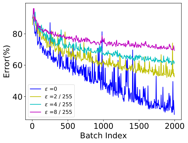
For ReLU networks, adversarially-trained models have been found to have sparser weights and intermediate activations [9], i.e., they have more dead neurons. Dead neurons are implicitly favored by adversarial training, because the output is independent of the input perturbation. Note that training fails when all the neurons in one layer are dead for all training instances. The model is then effectively broken into two parts by this dead layer: the preceding layers will no longer be trained because the gradients are all blocked; the following layers do not depend on the input and thus give constant outputs. In essence, training is then stuck in a parameter space that only includes constant classifiers. In practice, this usually happens when the model has small width and the value of $\epsilon$ is large.

Theorem 2 indicates that the gradients are non-vanishing in adversarial training and more likely to have large magnitude under large values of $\epsilon$. This is validated by Figure 2(d), in which we report the norm of the stochastic gradient $\|\triangledown_{\theta}\widehat{\mathcal{L}}_{\epsilon}(\theta)\|$ in the last 2000 mini-batch updates for CIFAR10 models. In vanilla training, the gradient is almost zero in the end, indicating that the optimizer finds a critical point. In this case $\|\triangledown_{\theta}\widehat{\mathcal{L}}_{\epsilon}(\theta)\|$ is dominated by the variance introduced by stochasticity. However, $\|\triangledown_{\theta}\widehat{\mathcal{L}}_{\epsilon}(\theta)\|$ increases with $\epsilon$. When $\epsilon$ is larger, $\|\triangledown_{\theta}\widehat{\mathcal{L}}_{\epsilon}(\theta)\|$ is also larger and non-vanishing, indicating that the model is still bouncing around the parameter space at the end of training.

The decreased gradient magnitude in the initial suboptimal region and the increased gradient magnitude in the final near-minimum region indicate that the adversarial loss landscape is not favorable to optimization when we train under large adversarial budgets. Additional results on MNIST models are provided in Figure 8 of Appendix C.2.1, where the same observations can be made.

To study the effective local Lipschitz constant of $\mathcal{L}_{\epsilon}(\theta)$, we analyze the Hessian spectrum of models trained under different values of $\epsilon$. It is known that the curvature in the neighborhood of model parameters is dominated by the top eigenvalues of the Hessian matrix $\triangledown^{2}\mathcal{L}_{\epsilon}(\theta)$. To this end, we use the power iteration method as in [50] to iteratively estimate the top 20 eigenvalues and the corresponding eigenvectors of the Hessian matrix. Furthermore, to discard the effect of the scale of function $\mathcal{L}_{\epsilon}(\theta)$ for different $\epsilon$, we estimate the scale of $\mathcal{L}_{\epsilon}(\theta)$ by randomly sampling $\theta$. We then normalize the top Hessian eigenvalues by the average value of $\mathcal{L}_{\epsilon}(\theta)$ on these random samples. In addition, we show the learning curve of $\mathcal{L}_{\epsilon}(\theta)$ on the training set during training in Figure 11 of Appendix C.2.2. It clearly show similar magnitude of $\mathcal{L}_{\epsilon}(\theta)$ for different values of $\epsilon$.

In Figure 4, we show the top 20 Hessian eigenvalues, both before and after normalization, of CIFAR10 models under different adversarial budgets. We also provide 3D visualizations of the neighborhood in the directions of the top 2 eigenvectors in Figure 12 of Appendix C.2.2. It is clear that the local effective second-order Lipschitz constant of the model obtained consistently increases with the value of $\epsilon$. That is, the minima found in $\mathcal{L}_{\epsilon}(\theta)$ are sharper under larger $\epsilon$.

To validate the claim in Section 3.2 that non-smoothness arises from abrupt changes of the adversarial examples, we study the similarity of adversarial perturbations generated by different model parameter values in a small neighborhood. Specifically, we perturb the model parameters $\theta$ in opposite directions to $\theta+a\mathbf{v}$ and $\theta-a\mathbf{v}$, where $\mathbf{v}$ is a unit vector and $a$ is a scalar. Let $\mathbf{x}^{\prime}_{a\mathbf{v}}$ and $\mathbf{x}^{\prime}_{-a\mathbf{v}}$ represent the adversarial examples generated by the corresponding model parameters. We then calculate the average cosine similarity between the perturbation $\mathbf{x}^{\prime}_{a\mathbf{v}}-\mathbf{x}$ and $\mathbf{x}^{\prime}_{-a\mathbf{v}}-\mathbf{x}$ over the training set.

The results on CIFAR10 models are provided in Figure 4. To account for the random start in PGD, we run each experiment $4$ times and report the average value. The variances of all experiments are smaller than $0.005$ and thus not shown in the figure. Note that, when $\mathbf{v}$ is a random unit vector, the robust error $\mathcal{E}_{\epsilon}(\theta)$ of the parameters $\theta\pm a\mathbf{v}$ on both the training and test sets remains unchanged for different values of $a$, indicating a flat landscape in the direction $\mathbf{v}$. The adversarial examples in this case are mostly similar and have very high cosine similarity. By contrast, if $\mathbf{v}$ is the top eigenvector of the Hessian matrix, i.e., the most curvy direction, then we see a sharp increase in the robust error $\mathcal{E}_{\epsilon}(\theta)$ when we increase $a$. Correspondingly, the cosine similarity between the adversarial perturbations is much lower, which indicates dramatic changes of the adversarial examples. We perform the same experiments on MNIST models in Appendix C.2.2 with the same observations.

References

- [1] Naveed Akhtar and Ajmal Mian. Threat of adversarial attacks on deep learning in computer vision: A survey. IEEE Access, 6:14410–14430, 2018.
- [2] Jean-Baptiste Alayrac, Jonathan Uesato, Po-Sen Huang, Alhussein Fawzi, Robert Stanforth, and Pushmeet Kohli. Are labels required for improving adversarial robustness? In Advances in Neural Information Processing Systems, pages 12192–12202, 2019.
- [3] Maksym Andriushchenko, Francesco Croce, Nicolas Flammarion, and Matthias Hein. Square attack: a query-efficient black-box adversarial attack via random search. arXiv preprint arXiv:1912.00049, 2019.
- [4] Anish Athalye, Nicholas Carlini, and David Wagner. Obfuscated gradients give a false sense of security: Circumventing defenses to adversarial examples. arXiv preprint arXiv:1802.00420, 2018.
- [5] Mislav Balunovic and Martin Vechev. Adversarial training and provable defenses: Bridging the gap. In International Conference on Learning Representations, 2020.
- [6] Yair Carmon, Aditi Raghunathan, Ludwig Schmidt, John C Duchi, and Percy S Liang. Unlabeled data improves adversarial robustness. In Advances in Neural Information Processing Systems, pages 11190–11201, 2019.
- [7] Djork-Arné Clevert, Thomas Unterthiner, and Sepp Hochreiter. Fast and accurate deep network learning by exponential linear units (elus). arXiv preprint arXiv:1511.07289, 2015.
- [8] Jeremy M Cohen, Elan Rosenfeld, and J Zico Kolter. Certified adversarial robustness via randomized smoothing. arXiv preprint arXiv:1902.02918, 2019.
- [9] Francesco Croce, Maksym Andriushchenko, and Matthias Hein. Provable robustness of relu networks via maximization of linear regions. arXiv preprint arXiv:1810.07481, 2018.
- [10] Francesco Croce and Matthias Hein. Reliable evaluation of adversarial robustness with an ensemble of diverse parameter-free attacks. arXiv preprint arXiv:2003.01690, 2020.
- [11] Laurent Dinh, Razvan Pascanu, Samy Bengio, and Yoshua Bengio. Sharp minima can generalize for deep nets. In Proceedings of the 34th International Conference on Machine Learning-Volume 70, pages 1019–1028. JMLR. org, 2017.
- [12] Felix Draxler, Kambis Veschgini, Manfred Salmhofer, and Fred A Hamprecht. Essentially no barriers in neural network energy landscape. arXiv preprint arXiv:1803.00885, 2018.
- [13] Stanislav Fort and Stanislaw Jastrzebski. Large scale structure of neural network loss landscapes. arXiv preprint arXiv:1906.04724, 2019.
- [14] Timur Garipov, Pavel Izmailov, Dmitrii Podoprikhin, Dmitry P Vetrov, and Andrew G Wilson. Loss surfaces, mode connectivity, and fast ensembling of dnns. In Advances in Neural Information Processing Systems, pages 8789–8798, 2018.
- [15] Mario Geiger, Stefano Spigler, Stéphane d’Ascoli, Levent Sagun, Marco Baity-Jesi, Giulio Biroli, and Matthieu Wyart. Jamming transition as a paradigm to understand the loss landscape of deep neural networks. Physical Review E, 100(1):012115, 2019.
- [16] Behrooz Ghorbani, Shankar Krishnan, and Ying Xiao. An investigation into neural net optimization via hessian eigenvalue density. arXiv preprint arXiv:1901.10159, 2019.
- [17] Xavier Glorot and Yoshua Bengio. Understanding the difficulty of training deep feedforward neural networks. In Proceedings of the thirteenth international conference on artificial intelligence and statistics, pages 249–256, 2010.
- [18] Ian J Goodfellow, Jonathon Shlens, and Christian Szegedy. Explaining and harnessing adversarial examples. arXiv preprint arXiv:1412.6572, 2014.
- [19] Akhilesh Gotmare, Nitish Shirish Keskar, Caiming Xiong, and Richard Socher. A closer look at deep learning heuristics: Learning rate restarts, warmup and distillation. arXiv preprint arXiv:1810.13243, 2018.
- [20] Sven Gowal, Krishnamurthy Dvijotham, Robert Stanforth, Rudy Bunel, Chongli Qin, Jonathan Uesato, Timothy Mann, and Pushmeet Kohli. On the effectiveness of interval bound propagation for training verifiably robust models. arXiv preprint arXiv:1810.12715, 2018.
- [21] Shupeng Gui, Haotao N Wang, Haichuan Yang, Chen Yu, Zhangyang Wang, and Ji Liu. Model compression with adversarial robustness: A unified optimization framework. In Advances in Neural Information Processing Systems, pages 1283–1294, 2019.
- [22] Kaiming He, Xiangyu Zhang, Shaoqing Ren, and Jian Sun. Delving deep into rectifiers: Surpassing human-level performance on imagenet classification. In Proceedings of the IEEE international conference on computer vision, pages 1026–1034, 2015.
- [23] Kaiming He, Xiangyu Zhang, Shaoqing Ren, and Jian Sun. Deep residual learning for image recognition. In Proceedings of the IEEE conference on computer vision and pattern recognition, pages 770–778, 2016.
- [24] Dan Hendrycks, Kimin Lee, and Mantas Mazeika. Using pre-training can improve model robustness and uncertainty. arXiv preprint arXiv:1901.09960, 2019.
- [25] Gao Huang, Yixuan Li, Geoff Pleiss, Zhuang Liu, John E Hopcroft, and Kilian Q Weinberger. Snapshot ensembles: Train 1, get m for free. arXiv preprint arXiv:1704.00109, 2017.
- [26] Kenji Kawaguchi. Deep learning without poor local minima. In Advances in neural information processing systems, pages 586–594, 2016.
- [27] Nitish Shirish Keskar, Dheevatsa Mudigere, Jorge Nocedal, Mikhail Smelyanskiy, and Ping Tak Peter Tang. On large-batch training for deep learning: Generalization gap and sharp minima. arXiv preprint arXiv:1609.04836, 2016.
- [28] Diederik P Kingma and Jimmy Ba. Adam: A method for stochastic optimization. arXiv preprint arXiv:1412.6980, 2014.
- [29] J Zico Kolter and Eric Wong. Provable defenses against adversarial examples via the convex outer adversarial polytope. arXiv preprint arXiv:1711.00851, 1(2):3, 2017.
- [30] Jason D Lee, Max Simchowitz, Michael I Jordan, and Benjamin Recht. Gradient descent converges to minimizers. arXiv preprint arXiv:1602.04915, 2016.
- [31] Hao Li, Zheng Xu, Gavin Taylor, Christoph Studer, and Tom Goldstein. Visualizing the loss landscape of neural nets. In Advances in Neural Information Processing Systems, pages 6389–6399, 2018.
- [32] Xingjun Ma, Yuhao Niu, Lin Gu, Yisen Wang, Yitian Zhao, James Bailey, and Feng Lu. Understanding adversarial attacks on deep learning based medical image analysis systems. Pattern Recognition, page 107332, 2020.
- [33] Aleksander Madry, Aleksandar Makelov, Ludwig Schmidt, Dimitris Tsipras, and Adrian Vladu. Towards deep learning models resistant to adversarial attacks. arXiv preprint arXiv:1706.06083, 2017.
- [34] Seyed-Mohsen Moosavi-Dezfooli, Alhussein Fawzi, Omar Fawzi, and Pascal Frossard. Universal adversarial perturbations. In Proceedings of the IEEE conference on computer vision and pattern recognition, pages 1765–1773, 2017.
- [35] Roman Novak, Yasaman Bahri, Daniel A. Abolafia, Jeffrey Pennington, and Jascha Sohl-Dickstein. Sensitivity and generalization in neural networks: an empirical study. In International Conference on Learning Representations, 2018.
- [36] Aditi Raghunathan, Jacob Steinhardt, and Percy Liang. Certified defenses against adversarial examples. arXiv preprint arXiv:1801.09344, 2018.
- [37] Leslie Rice, Eric Wong, and J Zico Kolter. Overfitting in adversarially robust deep learning. arXiv preprint arXiv:2002.11569, 2020.
- [38] Itay Safran and Ohad Shamir. On the quality of the initial basin in overspecified neural networks. In International Conference on Machine Learning, pages 774–782, 2016.
- [39] Hadi Salman, Greg Yang, Jerry Li, Pengchuan Zhang, Huan Zhang, Ilya Razenshteyn, and Sebastien Bubeck. Provably robust deep learning via adversarially trained smoothed classifiers. arXiv preprint arXiv:1906.04584, 2019.
- [40] Ludwig Schmidt, Shibani Santurkar, Dimitris Tsipras, Kunal Talwar, and Aleksander Madry. Adversarially robust generalization requires more data. In Advances in Neural Information Processing Systems, pages 5014–5026, 2018.
- [41] Ali Shafahi, Mahyar Najibi, Amin Ghiasi, Zheng Xu, John Dickerson, Christoph Studer, Larry S Davis, Gavin Taylor, and Tom Goldstein. Adversarial training for free! arXiv preprint arXiv:1904.12843, 2019.
- [42] Abhishek Sinha, Mayank Singh, Nupur Kumari, Balaji Krishnamurthy, Harshitha Machiraju, and Vineeth N Balasubramanian. Harnessing the vulnerability of latent layers in adversarially trained models. arXiv preprint arXiv:1905.05186, 2019.
- [43] Aman Sinha, Hongseok Namkoong, and John Duchi. Certifiable distributional robustness with principled adversarial training. In International Conference on Learning Representations, 2018.
- [44] Ivan Skorokhodov and Mikhail Burtsev. Loss surface sightseeing by multi-point optimization. arXiv preprint arXiv:1910.03867, 2019.
- [45] Christian Szegedy, Wojciech Zaremba, Ilya Sutskever, Joan Bruna, Dumitru Erhan, Ian Goodfellow, and Rob Fergus. Intriguing properties of neural networks. arXiv preprint arXiv:1312.6199, 2013.
- [46] Eric Wong, Leslie Rice, and J. Zico Kolter. Fast is better than free: Revisiting adversarial training. In International Conference on Learning Representations, 2020.
- [47] Eric Wong, Frank Schmidt, Jan Hendrik Metzen, and J Zico Kolter. Scaling provable adversarial defenses. In Advances in Neural Information Processing Systems, pages 8410–8419, 2018.
- [48] Cihang Xie and Alan Yuille. Intriguing properties of adversarial training. arXiv preprint arXiv:1906.03787, 2019.
- [49] Cihang Xie and Alan Yuille. Intriguing properties of adversarial training at scale. In International Conference on Learning Representations, 2020.
- [50] Zhewei Yao, Amir Gholami, Qi Lei, Kurt Keutzer, and Michael W Mahoney. Hessian-based analysis of large batch training and robustness to adversaries. In Advances in Neural Information Processing Systems, pages 4949–4959, 2018.
- [51] Shaokai Ye, Kaidi Xu, Sijia Liu, Hao Cheng, Jan-Henrik Lambrechts, Huan Zhang, Aojun Zhou, Kaisheng Ma, Yanzhi Wang, and Xue Lin. Adversarial robustness vs. model compression, or both. In The IEEE International Conference on Computer Vision (ICCV), volume 2, 2019.
- [52] Dinghuai Zhang, Tianyuan Zhang, Yiping Lu, Zhanxing Zhu, and Bin Dong. You only propagate once: Accelerating adversarial training via maximal principle. In Advances in Neural Information Processing Systems, pages 227–238, 2019.
- [53] Huan Zhang, Hongge Chen, Chaowei Xiao, Bo Li, Duane Boning, and Cho-Jui Hsieh. Towards stable and efficient training of verifiably robust neural networks. arXiv preprint arXiv:1906.06316, 2019.
- [54] Pu Zhao, Pin-Yu Chen, Payel Das, Karthikeyan Natesan Ramamurthy, and Xue Lin. Bridging mode connectivity in loss landscapes and adversarial robustness. In International Conference on Learning Representations, 2020.
Appendix A Theoretical Analysis
A.1 Binary Logistic Regression
In this section, we discuss binary logistic regression. In this case, and the logit function is , where is the only trainable parameter. If we use and to label both classes, then the overall loss function for a dataset is . Under the adversarial budget , the corresponding adversarial loss function is , where is the dual norm of . Since the magnitude of does not change the results of the classifier, we can assume without loss of generality. As a result, the adversarial loss function is