Towards Model-Agnostic Post-Hoc Adjustment for Balancing Ranking Fairness and Algorithm UtilityConference: Proceedings of the 27th ACM SIGKDD Conference on Knowledge Discovery and Data Mining; August 14–18, 2021; Virtual Event, Singapore.Proceedings of the 27th ACM SIGKDD Conference on Knowledge Discovery and Data Mining (KDD ’21), August 14–18, 2021, Virtual Event, SingaporePrice: 15.00ISBN: 978-1-4503-8332-5/21/08DOI: 10.1145/3447548.3467251CCS: Computing methodologies RankingCCS: Theory of computation Design and analysis of algorithmsCCS: Theory of computation Theory and algorithms for application domains

Machine learning algorithms have been widely applied in a variety of real-world applications including the high-stakes scenarios such as loan approvals, criminal justice, healthcare, etc. An increasing concern is whether these algorithms make fair decisions in these cases. For example, ProPublica reported that an algorithm used across the US for predicting a defendant’s risk of future crime produced higher scores to African-Americans than Caucasians on average (Angwin et al. 2016). This stimulates lots of research on improving the fairness of the decisions made by machine learning algorithms.

Existing works on fairness in machine learning have mostly focused on the disparate impacts of binary decisions informed by algorithms with respect to different groups formed from the protected variables (e.g., gender or race). Demographic parity requires the classification results to be independent of the group memberships. Equalized odds (Hardt et al. 2016) seeks for equal false positive and negative rates across different groups. Accuracy parity (Zafar et al. 2017) needs equalized error rates across different groups.

Another scenario that frequently involves computational algorithms is ranking. For example, Model for End-stage Liver Disease (MELD) score, which is derived from a simple linear model from several features, has been used for prioritizing candidates who need liver transplantation (Wiesner et al. 2003). Studies have found that women were less likely than men to receive a liver transplant within 3 years with the MELD score (Moylan et al. 2008). To quantify ranking fairness, Kallus et al. (Kallus and Zhou 2019) proposed xAUC, which measures the probability of positive examples of one group being ranked above negative examples of another group. Beutel et al. (Beutel et al. 2019a) proposed a similar definition pairwise ranking fairness (PRF), which requires equal probabilities for positive instances from each group ranked above all negative instances.

To address the potential disparity induced from risk scores, Kallus et al. (Kallus and Zhou 2019) proposed a post-processing approach that adjusts the risk scores of the instances in the disadvantaged group with a parameterized monotonically increasing function. This method is model agnostic and aims to achieve equal xAUC, but it does not consider algorithm utility (i.e., AUC) explicitly. Beutel et al. (Beutel et al. 2019a) studied the balance between algorithm utility and ranking fairness and proposed an optimization framework by minimizing an objective including the classification loss and a regularization term evaluating the absolute correlation between the group membership and pairwise residual predictions. Though this method considers both utility and fairness, is model-dependent and does not directly optimize PRF disparity but an approximated proxy.

In this paper, we develop a model agnostic post-processing framework, xOrder, to achieve ranking fairness and maintain the algorithm utility. Specifically, we show that both algorithm utility and ranking fairness are essentially determined by the ordering of the instances involved. xOrder makes direct adjustments of the cross-group instance ordering (while existing post-processing algorithms mostly aimed at adjusting the ranking scores to optimize the ordering). The optimal adjustments can be obtained through a dynamic programming procedure of minimizing an objective comprising a weighted sum of algorithm utility loss and ranking disparity. We theoretically analyze our method in two cases. If we focus on maximizing the utility, xOrder achieves a global optimal solution. While we care only about minimizing the disparity, it can have a relatively low bound of ranking disparity. The learned ordering adjustment can be easily transferred to the test data through linear interpolation.

We evaluate xOrder empirically on four popular benchmark data sets for studying algorithm fairness and two real-world electronic health record data repositories. The results show xOrder can achieve low ranking disparities on all data sets while at the same time maintaining good algorithm utilities. In addition, we compare the performance of xOrder with another post-processing algorithm when faced with the difference between training and test distributions. From the results, we find our algorithm can achieve robust performance when training and test ranking score distributions are significantly different. The source codes of xOrder are made publicly available at https://github.com/cuis15/xorder.

Algorithm fairness is defined as the disparities in the decisions made across groups formed by protected variables, such as gender and race. Many previous works on this topic focused on binary decision settings. Researchers have used different proxies as fairness measures which are required to be the same across different groups for achieving fairness. Examples of such proxies include the proportion of examples classified as positive (Calders et al. 2009; Calders and Verwer 2010), as well as the prediction performance metrics such as true/false positive rates and error rates (Dixon et al. 2018; Feldman et al. 2015; Hardt et al. 2016; Zafar et al. 2017; Kallus and Zhou 2018). A related concept that is worthy of mentioning here is calibration (Lichtenstein et al. 1981). A model with risk score $\operatorname{S}$ on input $\operatorname{X}$ to generate output $\operatorname{Y}$ is considered calibrated by group if for $\forall s\in[0,1]$, we have $\operatorname{Pr}(\operatorname{Y}=1|\operatorname{S}=s,\operatorname{A}=a)=\operatorname{Pr}(\operatorname{Y}=1|\operatorname{S}=s,\operatorname{A}=b)$ where $\mathrm{A}$ is the group variable (Chouldechova 2017). Recent studies have shown that it is impossible to satisfy both error rate fairness and calibration simultaneously when the prevalence of positive instances are different across groups (Kleinberg et al. 2016; Chouldechova 2017). Plenty of approaches have been proposed to achieve fairness in binary classification settings. One type of method is to train a classifier without any adjustments and then post-process the prediction scores by setting different thresholds for different groups (Hardt et al. 2016). Other methods have been developed for optimization of fairness metrics during the model training process through adversarial learning (Zemel et al. 2013; Louizos et al. 2015; Beutel et al. 2017; Madras et al. 2018; Zhang et al. 2018) or regularization (Kamishima et al. 2011; Zafar et al. 2015; Beutel et al. 2019b).

Ranking fairness is an important issue in applications where the decisions are made by algorithm produced ranking scores, such as the example of liver transplantation candidate prioritization with MELD score (Wiesner et al. 2003). This problem is related to but different from binary decision making (Narasimhan and Agarwal 2013; Menon and Williamson 2016). There are prior works formulating this problem in the setting of selecting the top-k items ranked based on the ranking scores for any k (Celis et al. 2017; Yang and Stoyanovich 2017; Zehlike et al. 2017; Geyik et al. 2019). For each sub-problem with a specific k, the top-k ranked examples can be treated as positive while the remaining examples can be treated as negative, so that these sub-problems can be viewed as binary classification problems. There are works trying to assign a weight to each instance according to the orders and study the difference of such weights across different groups (Singh and Joachims 2018; Singh and Joachims 2019). Our focus is the fairness on bipartite ranking, which seeks for a good ranking function that ranks positive instances above negative ones (Menon and Williamson 2016). Kallus et al. (Kallus and Zhou 2019) defined xAUC (Area under Cross-Receiver Operating Characteristic curve) as the probability of positive examples of one group being ranked above negative examples of another group. They require equal xAUC to achieve ranking fairness. Beutel et al. proposed a similar definition of pairwise ranking fairness(PRF) as the probability that positive examples from one group are ranked above all negative examples (Beutel et al. 2019a) and use the difference of PRF across groups as a ranking fairness metric. They further proved that some traditional fairness metrics (such as calibration and MSE) are insufficient for guaranteeing ranking fairness under PRF metric.

To address ranking fairness problem, Kallus et al. (Kallus and Zhou 2019) proposed a post-processing technique. They transformed the prediction scores in the disadvantaged group with a logistic function and optimized the empirical xAUC disparity by exhaustive searching on the space of parameters without considering the trade-off between algorithm utility and fairness. As the objective of the ranking problem is non-differentiable, there are theoretical and empirical works which propose to apply a differentiable objective to approximate the original non-differentiable objective (Vogel et al. 2020)  (Beutel et al. 2019a)  (Narasimhan et al. 2020). Vogel et al. propose to use a logistic function as smooth surrogate relaxations and provide upper bounds of the difference between the global optima of the original and the relaxed objectives. Narasimhan et al. reduced ranking problems to constrained optimization problems and proposed to solve the problems by applying an existed optimization framework proposed in  (Cotter et al. 2019). Beutel et al. proposed a pairwise regularization for the objective function (Beutel et al. 2019a). The regularization is computed as the absolute correlation between the residual prediction scores of the positive and negative example and the group membership of the positive example. However, PRF disparity is determined by judging whether a positive example is ranked above a negative one using an indicator function. The proposed pairwise regularization can be seen as an approximation of PRF disparity by replacing the indicator function with the residual prediction scores. This regularization does not guarantee ranking fairness under PRF metric. Moreover, it is difficult to apply this regularization to some learning methods such as boosting model (Freund et al. 2003). If we apply fairness regularization proposed by Beutal et al. to boosting model, it is challenging to reweight the samples during the boosting iterations, because the impact of increasing/decreasing the weight of the samples on fairness is difficult to control.

Suppose we have data ($\operatorname{X}$, $\operatorname{A}$, $\operatorname{Y}$) on features $\operatorname{X}\in\mathcal{X}$, sensitive attribute $\operatorname{A}\in\mathcal{A}$ and binary label $\operatorname{Y}\in\{0,1\}$. We are interested in the performance and the fairness issue of a predictive ranking score function $R$: $\mathcal{X}\times\mathcal{A}\rightarrow\mathbb{R}$. Here we focus on the case where $R$ returns an estimated conditional probability positive label corresponding to a given individual’s ranking score. We use $\mathrm{S}=R(\operatorname{X},\operatorname{A})\in[0,1]$ to denote the individual ranking score variable and the score $\mathrm{S}$ means the probability that the individual belongs to positive group.

Given $\operatorname{S}$, we can derive a binary classifier with a given threshold $\theta$, such that $\hat{\operatorname{Y}}_{\theta}=\mathbb{I}[\operatorname{S}\geq\theta]$ and $\mathbb{I}$ is the indicator function. To evaluate the performance of $R$, the receiver operator characteristic (ROC) curve is widely adopted with the false positive rate (FPR) on x-axis and the true positive rate (TPR) on y-axis as the threshold $\theta$ varies. The area under the ROC curve (AUC) quantitatively measures the quality of the learned scoring function $R$.

AUC can also be understood as the probability that a randomly drawn ranking score from the positive class is ranked above a randomly drawn score from the negative class (Hanley and McNeil 1982)

where $\operatorname{S}_{1}$ and $\operatorname{S}_{0}$ represent a ranking score of a random positive and negative sample. $n_{1}$ and $n_{0}$ correspond to the number of positives and negatives, respectively. Note that we dropped the group variable in the $R$ function because it is irrelevant to the measure of AUC (i.e., $\mathrm{X}_{i}$, $\mathrm{X}_{i}$ can be from any groups). The two group-level ranking fairness metrics can be measured by the following Cross-Area Under the Curve (xAUC) metric (Kallus and Zhou 2019).

From Eq.(2) we can see that xAUC measures the probability of a random positive sample in $a$ ranked higher than a random negative sample in $b$. Correspondingly, xAUC($b$,$a$) means $\operatorname{Pr}(\operatorname{S}_{1}^{b}>\operatorname{S}_{0}^{a})$, and the ranking disparity can be measured by

From Eq.(4) we can see that the PRF for group $a$ measures the probability of a random positive sample in $a$ ranked higher than a random negative sample in either $a$ or $b$. Then we can also define the following $\Delta$PRF metric to measure the ranking disparity

From above definitions we can see the utility (measured by AUC as in Eq.(1)) and fairness (measured by $\Delta$xAUC in Eq.(2) or $\Delta$PRF in Eq.(4)) of ranking function $R$ are essentially determined by the ordering of data samples induced by the predicted ranking scores. In the following, we use $\operatorname{p}^{a}$ and $\operatorname{p}^{b}$ to represent the data sample sequences in $a$ and $b$ with their ranking scores ranked in descending orders. That is, $\operatorname{p}^{a}=[\operatorname{p}^{a(1)},\operatorname{p}^{a(2)},...,\operatorname{p}^{a(n^{a})}]$ with $R(\operatorname{X}_{\operatorname{p}^{a(i)}},a)\geqslant R(\operatorname{X}_{\operatorname{p}^{a(j)}},a)$ if $0\leqslant i<j\leqslant n^{a}$, and $\operatorname{p}^{b}$ is defined in the same way, then we have the following definition.

One example of such cross-group ordering is:

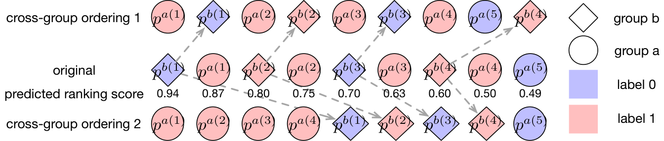
$o(\operatorname{p}^{a},\operatorname{p}^{b})$=$[\operatorname{p}^{a(1)},\operatorname{p}^{b(1)},\operatorname{p}^{a(2)},...,\operatorname{p}^{a(n^{a})},...,\operatorname{p}^{b(n^{b})}]$. From the above definitions we can see that we only need cross-group ordering $o(\operatorname{p}^{a},\operatorname{p}^{b})$ to estimate both algorithm utility measured by AUC and ranking fairness measured by either $\Delta$xAUC or $\Delta$PRF, i.e., we do not need the actual ranking scores. With this definition, we have the following proposition.

The proof of Proposition 1 is provided in Appendix. From proposition  4, if we only care about ranking fairness, we can achieve a relatively low disparity by a trivial method introduced in Appendix. Our proposal in this paper is to look for an optimal cross-group ordering $o^{*}(\operatorname{p}^{a},\operatorname{p}^{b})$, which can achieve ranking fairness and maximally maintain algorithm utility, through post-processing. We will use xAUC as the ranking fairness metric in our detailed derivations. The same procedure can be similarly developed for PRF based ranking fairness.

One important issue to consider is that the cross-group ordering that achieves the same level of ranking fairness is not unique. In Figure 1, we demonstrate an illustrative example with 9 samples showing that different cross-group ordering can result in different AUCs with the same $\Delta$xAUC. The middle row in Figure 1 shows the original predicted ranking scores and their induced sample ranking, which achieves a ranking disparity $\Delta\mathrm{xAUC}=0.75$. The top row shows one cross-group ordering with ranking disparity $\Delta\mathrm{xAUC}=0$ and algorithm utility $\mathrm{AUC}=0.56$. The bottom row shows another cross-group ranking with $\Delta\mathrm{xAUC}=0$ but $\mathrm{AUC}=0.83$.

The proof of this proposition is provided in Appendix.

To intuitively understand the post-processing process, we treat the cross-group ordering as a path from the higher ranked instances to lower ranked instances. With the same example shown in Figure 1, we demonstrate the original ordering of those samples induced by their predicted ranking scores (middle row of Figure 1) on the top of Figure 2(a), where the direction on the path indicates the ordering. The ordering corresponding to the bottom row of Figure 1 is demonstrated at the bottom of Figure 2(a).

With this analogy, the optimal cross-group ordering $o^{*}(\operatorname{p}^{a},\operatorname{p}^{b})$ can be achieved by a path finding process. The path must start from $\operatorname{p}^{a(1)}$ or $\operatorname{p}^{b(1)}$, and end with $\operatorname{p}^{a(n^{a})}$ or $\operatorname{p}^{b(n^{b})}$. Each instance in $\operatorname{p}^{a}$ and $\operatorname{p}^{b}$ can only appear once in the final path, and the orders of the instances in the final path must be the same as their orders in $\operatorname{p}^{a}$ and $\operatorname{p}^{b}$. The path can be obtained through a dynamic programming process. In particular, we first partition the entire decision space into a $(n^{b}+1)\times(n^{a}+1)$ grid. Each location $(i,j)~0\leqslant i\leqslant n^{a},0\leqslant j\leqslant n^{b}$ on the lattice corresponds to a decision step on determining whether to add $p^{a(i)}$ or $p^{b(j)}$ into the current path, which can be determined with the following rule:

where $\operatorname{p}^{a(:i)}$ represents the first $i$ elements in $\operatorname{p}^{a}$ ($\operatorname{p}^{a(:i-1)}$, $\operatorname{p}^{b(:j-1)}$ and $\operatorname{p}^{b(:j)}$ are similarly defined). $o^{*}(\operatorname{p}^{a(:i-1)},\operatorname{p}^{b(:j)})\textcircled{+}\operatorname{p}^{a(i)}$ means appending $\operatorname{p}^{a(i)}$ to the end of $o^{*}(\operatorname{p}^{a(:i-1)},\operatorname{p}^{b(:j)})$. The value of function $\widehat{\mathrm{G}}(o(\operatorname{p}^{a(:i)},\operatorname{p}^{b(:j)}))$ is defined as follows

in which $\widehat{\operatorname{G}}(o(\operatorname{p}^{a(:i)},\operatorname{p}^{b(:j)}))=\operatorname{G}(o(\operatorname{p}^{a},\operatorname{p}^{b}))$ in Eq. 16 when $i=n^{a},j=n^{b}$.

Figure 2(a) demonstrates the case of applying our rule to step $i=4,j=3$ in the example shown in Figure 1.

Algorithm 1 summarized the whole pipeline of identifying the optimal path. In particular, our algorithm calculates a cost for every point $(i,j)$ in the decision lattice as the value of the $\operatorname{\widehat{G}}$ function evaluated on the path reaching $(i,j)$ from $(0,0)$. Please note that the first row ($j=0$) only involves the instances in $a$, therefore the path reaching the points in this row are uniquely defined considering the within group instance order should be preserved in the path. The decision points in the first column ($i=0$) enjoy similar characteristics. After the cost values for the decision points in the first row and column are calculated, the costs values on the rest of the decision points in the lattice can be calculated iteratively until $i=n^{a}$ and $j=n^{b}$.

Algorithm 1 can also be viewed as a process to maximize the objective function in Eq.(6). It has $O(N^{2})$ time complexity as it is a 2-D dynamic programming process. Different $\lambda$ values trade-off the algorithm utility and ranking fairness differently and the solution Algorithm 1 converges to is a local optima. Moreover, we have the following proposition.

The proof of this theorem is provided in Appendix.

From the above process, we transfer the learned ordering from training set to test set by interpolation. We also try other operations to achieve interpolation (e.g. ranking uniform linear interpolation) and get similar experimental results.

In this paper, we investigate the problem of algorithmic fairness. Given an imperfect model, we propose a general post-processing framework, xOrder, to achieve a good balance between ranking fairness and model utility by direct adjustment to the cross group ranking orders. We formulate xOrder as an optimization problem and propose a dynamic programming process to solve it. Empirical results on both benchmark and real world medical data sets demonstrated that xOrder can achieve a low ranking disparity while keeping a maximum algorithm utility.