Engineering two-qubit mixed states with weak measurements

Introduction.—A generalized quantum measurement comprises a two-step protocol: (i) switching on, and later off, an interaction Hamiltonian, coupling the quantum system and the quantum detector, leading to a unitary evolution of the combined setup over a prescribed time interval; (ii) performing a projective measurement of the decoupled detector, which leads to a probabilistic quantum jump (von Neumann 2018; Wiseman and Milburn 2009; Wheeler and Zurek 1983). The detector readout provides information about the system’s state. Measurements are designated strong (projective) or weak, based on the system-detector interaction strength. The former collapses the system to one of the eigenstates of the measured observable. By contrast, generalized (a.k.a. weak) measurements may result in a slight nudge to the system state (Arthurs and Kelly 1965; Aharonov et al. 1988; Brun 2002; Svensson 2013; Patel and Kumar 2017). No matter how weak the measurement is, it always creates an unavoidable impact on the system state through its back-action (Korotkov 1999; Korotkov 2001). Traditionally, this measurement-induced back-action was considered an undesirable effect since the primary purpose of a measurement is to extract information about the system without perturbing it.

Following a disparate paradigm, one may employ the measurement-induced back-action on the system’s state as a means to control the system’s evolution, steering (Ste) it towards a predesignated pure target state (Pechen et al. 2006; Roa et al. 2006; Roa et al. 2007; Jacobs 2010; Ashhab and Nori 2010). A recent work (cf. (Roy et al. 2020) and references therein) analyzed a host of protocols utilizing “blind” measurements (Bli) for engineering pure target states in single- and many-body systems.

Traditionally, mixed states are not the objective of quantum steering. In practice, non-pure states may appear due to errors or noise of steering protocols. In a paradigmatic shift, we put them here as the target of steering, emphasizing the interest in and the value of mixed states. Their quantumness can be expressed through their discord Henderson and Vedral 2001; Ollivier and Zurek 2001; Modi et al. 2012; Hunt et al. 2019; *Kumar2020c; *Hunt2020. Discorded quantum states have been proposed as resources for various quantum information tasks: achieving quantum speedup (Datta et al. 2008; Lanyon et al. 2008), remote state preparation (Dakić et al. 2012), and quantum purification protocols (Bennett et al. 1996; Murao et al. 1998). Engineering predesignated mixed states is, therefore, a task of interest.

The present analysis introduces a measurement-based protocol which can be used to steer a two-qubit system to an arbitrary predesignated state (pure or mixed), independently of the system’s initial state (the latter is assumed unknown). We illustrate our protocol by considering a family of target states. These, depending on the protocol parameters, may be: (i) non-discorded and non-entangled (“classical”), (ii) discorded and non-entangled, or (iii) discorded and entangled, thus providing us with a smooth navigation tool from classical to fully quantum states.

The guiding principle of our protocol is as follows. Under sufficiently weak measurement, the system evolution can be described by a Lindbladian master equation. Such an equation will have at least one (and in the present case exactly one) steady state that is approached exponentially quickly. We design the protocol such that this steady state is the target state. We first recall a measurement-based protocol whose steady state is an arbitrarily chosen pure state (Roy et al. 2020). In order to generate a mixed state, we diagonalize the density matrix of the target state and juxtapose the protocols for stabilizing each of the density matrix’s pure eigenstates. In the explicit example we consider, we find that the rate of converging towards the target state does not significantly depend on its discord or degree of entanglement, so that our protocol is equally efficient independently of the target state’s usefulness for quantum information purposes.

General evolution under repeated blind measurements.—Consider a quantum system in state represented by the density matrix $\rho_{s}$ and a quantum detector prepared in state $\rho_{d}^{(0)}$. Before they interact, the joint system-detector state can be written as

In order to perform a measurement, the system interacts with the detector via an interaction Hamiltonian $H_{s-d}$; the joint system-detector state evolves as

where $U=\exp\left(-iH_{s-d}\tau\right)$, and $\tau$ is the interaction time. Subsequently the detector state is measured projectively, disentangling the composite system-detector state and generating a measurement back-action on the system state. When discarding (i.e., tracing out) the measurement readouts, a procedure we denote “blind measurement”, the effect of the back-action is represented through

Following each measurement step, the detector is reset to its initial state $\rho_{d}^{(0)}$, and then the same measurement procedure is repeated. This protocol gives rise to a non-trivial evolution of the system state.

Denoting the system-detector interaction time $\tau$, and taking the continuous time limit $\tau\rightarrow dt$, one arrives at the following differential equation for the system state evolution under blind measurements

Here $\mathcal{L}$ is the Liouvillian superoperator acting on the system state, and we dropped the terms $O(\tau^{2})$ on the r.h.s. The first term on the right-hand-side of the above equation generates unitary evolution of $\rho_{s}$, while the second term represents dissipative evolution and can be cast in the form of a Lindbladian. In other words, the above equation can be written as

where $\{\cdot,\cdot\}$ represents the anti-commutator, $H_{s}$ is the effective system Hamiltonian, and $L_{j}$ are the Lindblad jump operators acting on the system state. This way, the sequence of measurements influences the system state in a quasicontinuous manner and ultimately steers it to a steady state determined by the condition

Steering towards a pure target state.—We now recall the principles of measurement-based steering protocol of Ref. (Roy et al. 2020), focusing on the two-qubit case, at the center of our analysis. The protocol facilitates stabilizing the system in an arbitrary pure target state $\left|B_{1}\right\rangle$, corresponding to $\rho_{s}^{(T)}=|B_{1}\rangle\langle B_{1}|$.

To implement the protocol we first select three arbitrary states $\left|B_{2}\right\rangle$, $\left|B_{3}\right\rangle$, and $\left|B_{4}\right\rangle$, such that together with $\left|B_{1}\right\rangle$ they form an orthonormal basis in the four-dimensional Hilbert space of the two-qubit system. Three steps now follow: in the $k^{\text{th}}$ step, $k=1,2,3$, a measurement is performed with a system-detector coupling that is designed such that the measurement back-action steers the system away from $\left|B_{k+1}\right\rangle$. This is accomplished by choosing $H_{s-d}^{k}=J\left(|B_{1}\rangle\langle B_{k+1}|\otimes\sigma^{-}+h.c.\right)$, where the detector is a single qubit acted upon by the Pauli matrices $\sigma^{\pm}=\left(\sigma_{x}^{(d)}\pm i\sigma_{y}^{(d)}\right)/2$, and $J$ is the coupling strength (for simplicity it is the same in all the three steps). Before each measurement, the detector is initialized in $\rho_{d}^{(0)}=\left|\uparrow\right\rangle\left\langle\uparrow\right|$. With the duration of each step being $\tau$, the density matrix evolution over $dt=3\tau$ is given by

where $g=J^{2}\tau/3$, and the jump operators $L_{j}=(1-\delta_{1j})|B_{1}\rangle\langle B_{j}|$ (we introduced $L_{1}=0$ for completeness). It follows from Eq. (7) that

i.e., the system is steered towards the desired pure state.

It is instructive to understand the mechanism by which the above steering works. In each step, the system-detector interaction Hamiltonian $H_{s-d}^{k}$ steers the system in a two-dimensional subspace spanned by $|B_{1}\rangle$ and $|B_{k+1}\rangle$ from the state $|B_{k+1}\rangle$ to $|B_{1}\rangle$ without affecting the rest of $|B_{i}\rangle$ $(i\neq k+1)$. Since $H_{s-d}^{k}$ commutes with $|B_{1}\rangle\langle B_{1}|\otimes\rho_{d}^{(0)}$, the measurement does not disturb the system if it is in state $\left|B_{1}\right\rangle$, and the detector then remains in its initial state, $|\uparrow\rangle$. This makes $\left|B_{1}\right\rangle$ not just a steady state of the evolution, but a dark state in the terminology of Ref. (Diehl et al. 2008): once the system is in $\left|B_{1}\right\rangle$ it is not affected by the detectors. If the system is in $\left|B_{k+1}\right\rangle$, a transition to $\left|B_{1}\right\rangle$ (accompanied by the detector state flipping to $\left|\downarrow\right\rangle$) happens with probability $\sin^{2}J\tau$. Likewise, with probability $\cos^{2}J\tau$, the detector does not flip the state and the system remains in $\left|B_{k+1}\right\rangle$. Note that if the system is initially in a (coherent or incoherent) superposition of $\left|B_{1}\right\rangle$ and $\left|B_{k+1}\right\rangle$, both detector readouts affect the system state: $\left|\downarrow\right\rangle$ state of the detector implies the system has jumped from $\left|B_{k+1}\right\rangle$ to $\left|B_{1}\right\rangle$, while $\left|\uparrow\right\rangle$ implies a change of the weights of the superposition due to different probabilities of the $\uparrow$ readout depending on the system state (this is referred in the literature as a “null weak measurement” (Ruskov et al. 2007; Zilberberg et al. 2013; Zilberberg et al. 2014; Gebhart et al. 2020) or by a number of different names (Elitzur and Dolev 2001; Paraoanu 2006; Xu et al. 2011)). Averaging over the possible detector readouts and taking the limit $J\tau\ll 1$, one obtains the master equation (7).

Steering towards a mixed target state.—We now focus on the key result of the paper: steering the two-qubit system to a desired mixed state. Any mixed target state $\rho_{s}^{(T)}$ has a spectral decomposition (Nielsen and Chuang 2010)

where $\left|B_{i=1,...,4}\right\rangle$ form an orthonormal basis in the two-qubit Hilbert space, and $p_{i}\geq 0$ is the probability of the system being in the corresponding $\left|B_{i}\right\rangle$ state, so that $\sum_{i=1}^{4}p_{i}=1$. The protocol described in the previous section can be used to steer the system to $\left|B_{1}\right\rangle$. Furthermore, by exchanging the roles of $\left|B_{1}\right\rangle$ and one of $\left|B_{i\neq 1}\right\rangle$, the protocol steers the system to the corresponding $\left|B_{i}\right\rangle$. We now show that combining the four protocols, each steering the system to one of $\left|B_{i}\right\rangle$, with appropriate coupling strengths, $J\rightarrow J_{i}$, allows to stabilize the mixed state in Eq. (9).

A schematic experimental setup for this complex protocol is presented in Fig. 1. Each part of the protocol, steering the system towards one of the $\left|B_{i}\right\rangle$ lasts $3\tau$. Consequently, the density matrix evolution for $dt=4\times 3\tau=12\tau$ is described by

where $g_{i}=J_{i}^{2}\tau/12$ and $L_{j}^{(i)}=(1-\delta_{ij})|B_{i}\rangle\langle B_{j}|$. Equation (10) has a unique steady state,

We note that choosing

where $j=1,2,3,4$ and $\bar{g}=\sum_{i=1}^{4}g_{i}$, stabilizes the desired target state in Eq. (9). Therefore, measurement-based steering towards an arbitrary mixed state requires diagonalizing the density matrix of the latter, bringing the state to the form (9), and concurrent utilization of the four protocols, each stabilizing one of the pure eigenstates which make up the mixed-state density matrix.

We emphasize that the simple-looking result of Eq. (12) is highly non-trivial. Indeed, for arbitrary four Lindbladians $\tilde{\mathcal{L}}_{i}$ such that $\tilde{\mathcal{L}}_{i}[|B_{i}\rangle\langle B_{i}|]=0$, one cannot guarantee that $\sum_{i}g_{i}\tilde{\mathcal{L}}_{i}[\sum_{j}g_{j}|B_{j}\rangle\langle B_{j}|]=\sum_{i,j}g_{i}g_{j}\tilde{\mathcal{L}}_{i}[|B_{j}\rangle\langle B_{j}|]=0$. The fact that this holds in our case is a special feature of the measurements we employ here (i.e., of the Lindbladians describing the measurement-induced evolution). Employing other types of measurements may also allow for stabilizing arbitrary states, however, the relation between $g_{j}$ and $p_{j}$ may not be as simple as Eq. (12).

If we record the detector’s readouts, the dynamics of the system subject to our protocol can be understood as follows: The limit of weak measurement addressed here, $J_{i}\tau\ll 1$, implies that a detector click (one of the detectors flipping its state to $\left|\downarrow\right\rangle$ during the measurement) is a rare event. It follows that the system, initially prepared in a possibly coherent superposition of different $\left|B_{i}\right\rangle$, will experience coherence-preserving dynamics induced by a “no-click” back-action for a long time $\sim\bar{g}^{-1}$ (this is akin to “null weak measurements” (Ruskov et al. 2007; Zilberberg et al. 2013; Zilberberg et al. 2014; Gebhart et al. 2020)). Eventually, a click will register, bringing the system to one of the $\left|B_{i}\right\rangle$ states and destroying coherence between different $\left|B_{i}\right\rangle$ components. From this point on, the no-click dynamics does not affect the system state, while rare clicks make it jump between different $\left|B_{i}\right\rangle$ states. The system spending random amounts of time in different $\left|B_{i}\right\rangle$ results in the average state given by Eq. (9). Notably, the system, while being on average in the target state, probabilistically jumps among the constituent pure states $\left|B_{i}\right\rangle$, which is manifested by occasional detector clicks. In other words, a mixed target state in our protocol is a steady state but not a dark state.

Steering to “classical” vs “quantum” states.—We now illustrate our protocol with an example where the system can be steered into a family of states which can be classical or quantum depending on the measurement couplings employed. Consider the following two-qubit state,

where $|\psi^{\pm}\rangle=\frac{1}{\sqrt{2}}\left(|\uparrow\downarrow\rangle\pm|\downarrow\uparrow\rangle\right),$ and

Here $\alpha$ and $\beta$ are two independent parameters such that $0\leq\alpha,\beta\leq 1$, and the coefficients $p_{i}$ correspond to the $p_{i}$ in Eq. (9). This state may or may not have quantum correlations depending on $\alpha$ and $\beta$. For example, using Peres-Horodecki criterion (Peres 1996; Horodecki et al. 1996), one shows that $\tilde{\rho}$ is separable (not entangled) if and only if $\alpha\geq\frac{3\beta-1}{3\beta+1}$.

Quantum correlations are commonly quantified via concurrence (a measure of entanglement) (Wootters 1998; Modi et al. 2012) and quantum discord (Henderson and Vedral 2001; Ollivier and Zurek 2001; Modi et al. 2012; Hunt et al. 2019). Calculating discord $\mathcal{Q}$ and concurrence $\mathcal{C}$ for an arbitrary state is a challenging task, but for the state in Eq. (13) both of them can be calculated analytically (Wootters 1998; Luo 2008; Ali et al. 2010; Modi et al. 2012). They are respectively given by

and

Note that the discord $\mathcal{Q}(\tilde{\rho})$ is only zero when: (i) $\alpha=1$ or (ii) $\beta=0$, while the concurrence $\mathcal{C}(\tilde{\rho})$ exhibits a sharp change of behavior at finite $\alpha$ and $\beta$, cf. Fig. 2. The state $\tilde{\rho}$ can thus be purely classical (both discord and concurrence vanish), discorded (concurrence vanishes), or entangled (concurrence and discord are both non-zero) depending on the parameters $\alpha$ and $\beta$.

We may generate $\tilde{\rho}$ using the protocol described above. First, the target state density matrix should be diagonalized. It is evident from Eq. (13) that the eigenbasis of $\tilde{\rho}$ is

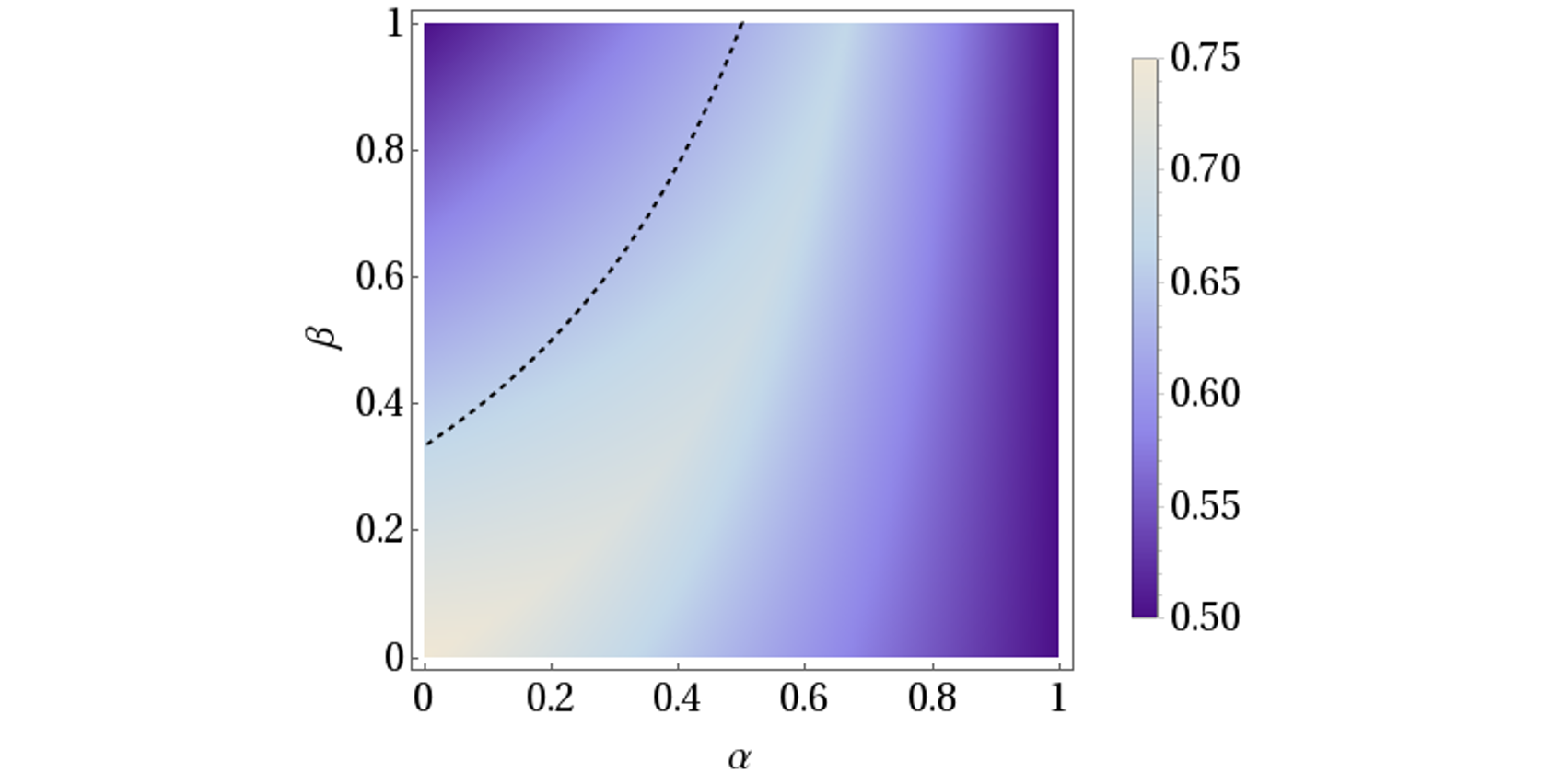
Using Eq. (12), one obtains that the couplings $g_{i}$ in Eq. (10) are $g_{i}=\bar{g}\,p_{i},$ where $\bar{g}=\sum_{i}g_{i}$ characterizes the total strength of all measurements employed. Figure 3 illustrates the time evolution of the two-qubit system as it is steered from an initial state to the target state $\tilde{\rho}$. Deviations from the target state decay exponentially in time; the decay rates are determined by the real parts of the non-zero eigenvalues of the Liouvillian superoperator $\mathcal{L}$, cf. Eq. (10). The smallest of the decay rates is referred to as the convergence rate; it is determined by the inverse of the Liouvillian gap—the smallest in magnitude real part of all non-zero eigenvalues. The dependence of the convergence rate on the target state is presented in Fig. 4. Note that the dependence on $\alpha$ and $\beta$ is not too strong, implying that our protocol works equally well for both entangled and non-entangled states, as well as for states in the vicinity of the transition between the two regions.

Discussion.—We have proposed a measurement-based protocol that can generate any two-qubit state by design (pure or mixed), starting from an arbitrary unknown initial state. We illustrate the protocol with an example, in which the target state can be classical, discorded, or entangled, depending on relative strengths of the measurements employed in the protocol.

Note that conventional studies of open system evolution (e.g., (Gao 1997; Prosen 2011; Albert and Jiang 2014)) are concerned with finding the steady state of a given Liouvillian. By contrast, here we are concerned with stabilizing a predesignated state ("target state"), i.e., finding the evolution protocol (Liouvillian) for which our target state is the steady state. We also note that our approach is distinct from drive-and-dissipation schemes (Wu et al. 2007; Diehl et al. 2008; Kraus et al. 2008; Roncaglia et al. 2010; Pechen 2011; Diehl et al. 2011; Murch et al. 2012; Bardyn et al. 2013; Leghtas et al. 2013; Liu et al. 2016; Goldman et al. 2016; Lu et al. 2017; Huang et al. 2018), where environment is employed to relax the system to a desired state. The two crucial distinctions here are: (a) the relaxation is induced by measurements, implying the possibility to use the measurement readouts to confirm the system’s desired behavior (and, possibly, hasten the convergence towards the target state); (b) our system does not have a Hamiltonian (no “drive”).

Our protocol can be implemented in a variety of experimental platforms. The main ingredient of our protocol, blind measurement stabilizing the system at a specific pure state, is particularly natural for implementation in cold-ion systems (Ben Av et al. 2020). The nature of cold-ion experiments does not allow for registering individual measurement readouts in order to verify the protocol behavior. This can, however, be done by working with superconducting “artificial atoms” (Vijay et al. 2011; Minev et al. 2019).

An interesting future direction concerns stabilizing $N$-qubit mixed states. Stabilizing $N$-qubit pure states in an efficient manner is already a challenging problem, which, however, has been solved for the restricted class of tensor-network states (Kraus et al. 2008; Verstraete et al. 2009; Roy et al. 2020). Stabilizing $N$-qubit mixed states turns out to be an even more challenging problem still under research (Bondarenko and Osborne 2018). Our two-qubit protocol may be a useful block in future $N$-qubit protocols.