Point-mass sensitivity of gravimetric satellitesJournal: Advances in Space Research

Robert Spero Address: robert.spero@jpl.nasa.gov
Jet Propulsion Laboratory, Pasadena, CA 91109

Abstract

Frequency-domain expressions are found for gradiometer and satellite-to-satellite tracking measurements of a point source on the surface of the Earth. The maximum signal-to-noise ratio as a function of noise in the measurement apparatus is computed, and from that the minimum detectable point mass is inferred. A point mass of magnitude $M_{3}={\text{\unboldmath$\mathrm{100}$}}\,\text{\unboldmath$\mathrm{Gt}$}$ gives a signal-to-noise ratio of 3 when a GOCE-like gradiometer passes directly over the mass. On the satellite-to-satellite tracking mission GRACE-FO $M_{3}={\text{\unboldmath$\mathrm{1{.}3}$}}\,\text{\unboldmath$\mathrm{Gt}$}$ for the microwave instrument and $M_{3}={\text{\unboldmath$\mathrm{0{.}5}$}}\,\text{\unboldmath$\mathrm{Gt}$}$ for the laser ranging interferometer. The sensitivity of future GRACE-like missions with different orbital parameters and improved accelerometer sensitivity is explored, and the optimum spacecraft separation for detecting point-like sources is found. The future-mission benefit of improving the accelerometer sensitivity for measurement of non-gravitational disturbances is shown by the resulting reduction of $M_{3},$ to as small as $\mathrm{7}$ $\mathrm{Mt}$ for $\mathrm{500}$ $\mathrm{km}$ orbital altitude and optimized satellite separation of $\mathrm{900}$ $\mathrm{km}$ .

1 Introduction

A global gravity map is the principal data product of satellite gravity missions. Previously CHAMP (Reigber et al., 2003), GRACE (Tapley et al., 2004), and GOCE (Drinkwater et al., 2006) collected data to map the Earth’s gravity, and GRAIL (Konopliv et al., 2013) measured the Moon’s gravity. Currently GRACE Follow-On (GRACE-FO, Landerer et al., 2020) is extending the GRACE data record, with increased ranging precision afforded by its laser ranging interferometer (LRI, Abich et al., 2019).

As pointed out by Watkins et al., 2015, the most commonly used method of analyzing satellite gravity data is based on global gravity fields expressed in terms of spherical harmonic basis functions. An alternative to spherical harmonics is the mass concentration, or mascon, model. Starting with Wong et al., 1971, the mascon approach was applied to single-satellite lunar orbital measurements to infer the surface gravity of the moon. Mascons can be modeled as many discrete sources (Pollack, 1973, Watkins et al., 2005) that cover the globe, or used to solve for regional fields. Han, 2013 applied mascons to GRAIL data to solve for regional fields of the Moon.

Though they differ slightly in assumptions and results, the spherical harmonic and mascon methods are constructed to answer the same question: what is the gravity field that is most consistent with measurements? Here we address a different question: what is the limit to measurement precision of a point-like mass on the surface? This is an artificial model, a single mascon, that is not directly applicable to the geodetic agenda of measuring the Earth’s gravity. We do not attempt to replicate the global gravity-field inversion achieved by the usual many-mascon analysis. Rather, the motivation for this analysis is twofold: to provide a single-number figure of merit, namely the minimum detectable isolated point mass perturbation, and to find the optimal filter for such a detection. The minimum detectable mass $M_{3}$ is defined as the point mass that a gives a signal-to-noise ratio $\rho=3$ in a single orbital pass directly over the point mass. It is calculated by applying the Wiener optimal filter to the problem of detecting a signal of known waveform, against a background specified by instrument noise power spectral density (Wainstein and Zubakov, 1970). A comparison of $M_{3}$ for different orbital configurations and instrument sensitivities guides the design of future missions. Additionally, we find the optimum satellite separation in GRACE-like missions for a specified instrument noise power spectral density.

2 Gradiometer Mass Sensitivity

Consider a gradiometer flying directly over a point mass $M$ at altitude $h,$ Figure 1 left.

Refer to caption — Fig. 1: Measurement of gravitational field from a point mass $M$ at along-track distance $x$ , altitude $h,$ and velocity $v.$ Left: Vertical gradient $g_{z}.$ Right: Differential acceleration $a_{R}$ between spacecraft 1 and 2 with average separation $L$ .

At orbital altitude $h={\text{\unboldmath$\mathrm{330}$}}\,\text{\unboldmath$\mathrm{km}$},$ the along-track velocity $v$ is the orbital velocity $v_{o}={\text{\unboldmath$\mathrm{7{.}7}$}}\,\text{\unboldmath$\mathrm{km/s}$}$ and the along-track distance $x$ changes at approximately constant rate, $x=v_{o}t.$ The acceleration at the spacecraft in the vertical, $z$ direction is $a_{z}=-GMz/(x^{2}+z^{2})^{3/2},$ and the gradient in the $z$ direction is $g_{z}=da_{z}/dz=GM[3z^{2}(x^{2}+z^{2})^{-5/2}-(x^{2}+z^{2})^{-3/2}].$ $G=$ Newton’s constant of gravitation. Substituting $z\rightarrow h$ and $x\rightarrow v_{o}t$ ,

g_{z}(t)=\kappa_{g}M\left[3(1+[f_{h}t]^{2})^{-5/2}-(1+[f_{h}t]^{2})^{-3/2}\right]

(1)

where $\kappa_{g}M=GM/h^{3}={\text{\unboldmath$\mathrm{1{.}85{}\times{}10^{-3}}$}}\,\text{\unboldmath$\mathrm{mE}$}$ with $M={\text{\unboldmath$\mathrm{1}$}}\,\text{\unboldmath$\mathrm{Gt}$}$ and $f_{h}=v_{o}/h={\text{\unboldmath$\mathrm{23}$}}\,\text{\unboldmath$\mathrm{mHz}$};\ {\text{\unboldmath$\mathrm{1}$}}\,\text{\unboldmath$\mathrm{mE}$}={\text{\unboldmath$\mathrm{1{}\times{}10^{-12}}$}}\,\text{\unboldmath$\mathrm{s^{-2}}$}.$ At $t=0$ , when the gradiometer is directly above the source mass, the gradient reaches its maximum value $g_{z}=2\kappa_{g}M.$ At $x=\pm\sqrt{2}h,\ g_{z}=0.$

The Fourier transform of $p(t)$ is defined by ${\mathcal{F}}[p(t)]\equiv p(f)=\int_{-\infty}^{\infty}dt\,p(t)\exp(-2\pi ift).$ Applying the Fourier transform to $g_{z}(t)$ :

g_{z}(f)=\kappa_{g}M\frac{4\pi f}{f_{h}^{2}}\left[K_{1}\left(\frac{2\pi f}{f_{h}}\right)+\frac{2\pi f}{f_{h}}K_{0}\left(\frac{2\pi f}{f_{h}}\right)\right]

(2)

where $K_{n}$ is the modified Bessel function of the second kind, order $n$ . From Abramowitz and Stegun, 1964, Section 9.7.2, $K_{n}(z)\sim\sqrt{\pi/(2z)}e^{-z},$ where $\sim$ indicates approximately equal for large $z.$ At frequency $f\gg f_{h},$ the measurement response is attenuated approximately exponentially with $e$ -folding frequency $f_{h}/(2\pi)={\text{\unboldmath$\mathrm{3{.}7}$}}\,\text{\unboldmath$\mathrm{mHz}$}.$ This corresponds to harmonic order $N=f_{h}/(2\pi f_{1})=20,$ where $f_{1}={\text{\unboldmath$\mathrm{0{.}183}$}}\,\text{\unboldmath$\mathrm{mHz}$}$ is the orbital frequency.

The signal-to-noise ratio $\rho$ depends on the signal and the power spectral density of the gradiometer noise, $S_{g}(f).$ Define the frequency-dependent signal-to-noise-ratio density SNRD as

W_{g_{z}}(f)=\frac{|g_{z}(f)|^{2}}{S_{g}(f)}.

(3)

In general, $\rho$ depends on what filtering is applied to the instrument output. After Flanagan and Hughes, 1998, with optimum filtering the maximum signal-to-noise ratio per unit source mass $\rho^{\prime}$ is

\rho^{\prime}=\sqrt{4\int_{0}^{\infty}W_{g_{z}}^{\prime}(f)df}.

(4)

Prime superscripts indicate quantities normalized by the source mass: $\rho^{\prime}=\rho/M$ and $W^{\prime}_{g_{z}}(f)=W_{g_{z}}(f)/M^{2}.$ It follows that the minimum detectable point mass with $\rho=3$ is

M_{3}=\frac{3}{\sqrt{4\int_{0}^{\infty}W^{\prime}_{g_{z}}(f)df}}.

(5)

The lower panel of Figure 2 shows $M_{3}$ as a function of orbital altitude $h$ for a gradiometer limited by white spectral noise $S_{g}(f)={\text{\unboldmath$\mathrm{1}$}}\,\text{\unboldmath$\mathrm{mE/\sqrt{\mathrm{Hz}}}$}$ (approximated value for GOCE from Touboul et al., 1999, Touboul et al., 1999a). At $h={\text{\unboldmath$\mathrm{330}$}}\,\text{\unboldmath$\mathrm{km}$},\ M_{3}={\text{\unboldmath$\mathrm{100}$}}\,\text{\unboldmath$\mathrm{Gt}$}$ and the minimum observable gradient at the peak time $t=0$ is $2\kappa_{g}M={\text{\unboldmath$\mathrm{0{.}37}$}}\,\text{\unboldmath$\mathrm{mE}$}.$

3 Sensitivity of GRACE-like measurements

The measurement configuration and signal parameters for the low-low satellite-to-satellite tracking (SST) of GRACE and GRACE-FO are shown in Figure 1, right. The primary signal is the along-track differential position of the spacecraft, measured by microwave ranging or laser interferometry.

3.1 Single Spacecraft Acceleration

For simplicity, the Flat-Earth approximation (Tapley, 1997) is used. This approximation neglects centrifugal acceleration, which introduces an error of less than 20% at Fourier frequencies greater than $\mathrm{2}$ $\mathrm{mHz}$ (Ghobadi-Far et al., 2018, Figure 1; Müller, 2017, Figure 1.7). In this approximation, the acceleration on spacecraft 1 flying over point mass $M$ at along-track distance $x$ is $a_{1}=-GMx/(h^{2}+x^{2})^{3/2}.$

Define the acceleration per unit source mass, $a^{\prime}_{1}=a_{1}/M.$ Then

a^{\prime}_{1}=-\frac{Gtv_{o}}{(h^{2}+v_{o}^{2}t^{2})^{3/2}}

(6)

Converting to frequency space,

a^{\prime}_{1}(f)=\mathcal{F}[a^{\prime}_{1}(t)]=\frac{4\pi ifGK_{0}\left(\frac{2\pi f}{f_{h}}\right)}{v^{2}_{o}}.

(7)

3.2 Range Acceleration Signal

The acceleration experienced by spacecraft 2 is the same as spacecraft 1 at distance $L$ , but delayed by $\tau=L/v_{o}.$ The resulting (along-track) range acceleration between the spacecraft (Figure 3, left) is similar to what Han, 2013 computed for the response of the GRAIL spacecraft to regional lunar gravity. The peak range acceleration $a_{R}^{p}$ is

a_{R}^{p}=\frac{GL}{\left(h^{2}+(L/2)^{2}\right)^{3/2}}M\equiv\kappa_{R}M,

(8)

where $\kappa_{R}=GL(h^{2}+(L/2)^{2})^{-3/2}.$

Using the identity $\mathcal{F}(\text{delay }\tau)=\exp(-2\pi if\tau)$ , the range acceleration in the frequency domain, $a_{R}(f),$ is given by

	$\displaystyle a^{\prime}_{R}(f)$	$\displaystyle=$	$\displaystyle a^{\prime}_{1}(f)(1-e^{-2\pi if\tau})$		(9)
	$\displaystyle\|a^{\prime}_{R}(f)\|$	$\displaystyle=$	$\displaystyle 2\|a^{\prime}_{1}(f)\sin(\pi f\tau)\|$		(10)

That is, in the frequency domain the range acceleration is the single-satellite acceleration multiplied by $2|\sin(\pi f\tau)|.$ For $f\ll 1/\tau,$ $|a_{R}(f)|~\propto L$ , which is the response for the spacecraft pair acting as a gradiometer. The response departs from that of a gradiometer at large $L,$ most conspicuously in the form of high-frequency nulls where the signal vanishes. The first null is at $f_{\mathrm{null}}=1/\tau={\text{\unboldmath$\mathrm{38}$}}\,\text{\unboldmath$\mathrm{mHz}$}$ for low-Earth orbit and $L={\text{\unboldmath$\mathrm{200}$}}\,\text{\unboldmath$\mathrm{km}$}$ , as recognized by Wolff, 1969. In degree-variance evaluations of measurement sensitivity, the first null is expressed as a maximum in geoid height error at degree $N=f_{\text{null}}/f_{1}=216$ for $L={\text{\unboldmath$\mathrm{200}$}}\,\text{\unboldmath$\mathrm{km}$},$ and $N=86$ for $L={\text{\unboldmath$\mathrm{500}$}}\,\text{\unboldmath$\mathrm{km}$},$ where $f_{1}=$ orbital frequency = $\mathrm{0{.}176}$ $\mathrm{mHz}$ .

From Equations 7 and 10,

|a^{\prime}_{R}(f)|=\frac{8\pi fG}{v^{2}_{o}}\left|K_{0}\left(\frac{2\pi f}{f_{h}}\right)\right|\left|\sin\left(\frac{2\pi f}{f_{L}}\right)\right|,

(11)

where

$\displaystyle v_{o}=$	orbital velocity	$\displaystyle=$	$\mathrm{7{.}6}$ $\mathrm{km/s}$
$\displaystyle h=$	orbital altitude	$\displaystyle=$	$\mathrm{500}$ $\mathrm{km}$
$\displaystyle L=$	spacecraft separation	$\displaystyle=$	$\mathrm{200}$ $\mathrm{km}$
$\displaystyle f_{h}=$	$\displaystyle\frac{v_{o}}{h}$	$\displaystyle=$	$\mathrm{15{.}2}$ $\mathrm{mHz}$
$\displaystyle f_{L}=$	$\displaystyle\frac{v_{o}}{L/2}$	$\displaystyle=$	$\mathrm{76}$ $\mathrm{mHz}$
$\displaystyle\tau=$	$\displaystyle\frac{L}{v_{o}}$	$\displaystyle=$	$\mathrm{26}$ $\mathrm{s}$
$\displaystyle\kappa_{R}=$	$\displaystyle\frac{GL}{\left(h^{2}+(L/2)^{2}\right)^{3/2}}$	$\displaystyle=$	$\displaystyle{\text{\unboldmath$\mathrm{0{.}101}$}}\,\text{\unboldmath$\mathrm{nm/s^{2}/Gt}$}.$

These numerical values apply to GRACE-FO. The approximately exponential attenuation with frequency of $|a_{R}(f)|$ has $e$ -folding frequency $\mathrm{2{.}5}$ $\mathrm{mHz}$ , corresponding to harmonic order $N=14.$

To explore the valid realm of the point-mass approximation, Figure 3 shows the range acceleration signal from a square-shaped planar mass of side length S, computed by numerical integration. The S=1 km result is in agreement with the point-mass analytical calculation, which is valid at the 20% level for sources as large as S=300 km. Henceforth, we restrict our analysis to the signal from a point source.

Equation 11 gives the measurement impulse response; that is, the range acceleration frequency response to a point mass input. This facilitates the direct comparison of signal and noise amplitudes as computed in the following section, and yields an expression for the minimum detectable mass for GRACE-like measurements of point source perturbations to surface gravity.

3.3 Noise and Mass Sensitivity

Consider the range measurement made by the laser ranging interferometer (LRI) on GRACE-FO. Assuming the measurement resolution is limited by the thermal noise of the laser reference cavity (Numata et al., 2004), the displacement noise root power spectral density (rpsd) $\tilde{x}_{\text{LRI}}$ and strain rpsd $\tilde{x}_{\text{LRI}}/L$ are given by

\tilde{x}_{\text{LRI}}(f)/L=x_{c}/\sqrt{f},

(12)

where $x_{c}$ is a constant. For the LRI (Abich et al., 2019), $x_{c}={\text{\unboldmath$\mathrm{1{}\times{}10^{-15}}$}}\,\text{\unboldmath$\mathrm{}$}.$ The rpsd of the LRI range acceleration noise is

\sqrt{S_{\text{LRI}}(f)}=(2\pi f)^{2}\cdot\tilde{x}_{\text{LRI}}(f).

(13)

Take for the accelerometer measurement noise rpsd on a single satellite of GRACE and GRACE-FO (Touboul et al., 1999)

\sqrt{S_{\mathrm{ACC_{1}}}(f)}=\tilde{a}_{0}\sqrt{1+\left(\frac{f_{k}}{f}\right)^{2}}.

(14)

Estaimates of $\tilde{a}_{0}$ and $f_{k}$ range from $\mathrm{3{}\times{}10^{-11}}$ $\mathrm{m/s^{2}/\sqrt{\text{Hz}}}$ and $\mathrm{10}$ $\mathrm{mHz}$ , respectively (Hauk and Wiese, 2020) to $\mathrm{1{}\times{}10^{-10}}$ $\mathrm{m/s^{2}/\sqrt{\text{Hz}}}$ and $\mathrm{5}$ $\mathrm{mHz}$ , respectively (Christophe et al., 2010, Conklin and Nguyen, 2017) . We take as a compromise $\tilde{a}_{0}={\text{\unboldmath$\mathrm{7{}\times{}10^{-11}}$}}\,\text{\unboldmath$\mathrm{m/s^{2}/\sqrt{\text{Hz}}}$}$ and $f_{k}={\text{\unboldmath$\mathrm{5}$}}\,\text{\unboldmath$\mathrm{mHz}$}.$ Assuming that the acceleration measurements on the two satellites are uncorrelated, the total accelerometer noise is double: $S_{\mathrm{ACC}}=2S_{\mathrm{ACC_{1}}}.$

Improved accelerometers in future missions (Christophe et al., 2010, Conklin and Nguyen, 2017) may have $\tilde{a}_{0}={\text{\unboldmath$\mathrm{7{}\times{}10^{-13}}$}}\,\text{\unboldmath$\mathrm{m/s^{2}/\sqrt{\text{Hz}}}$}.$

The total instrument noise power spectral density is

S_{a}=S_{\text{ACC}}+S_{\text{LRI}}.

(15)

Figure 4 shows $\sqrt{S_{a}}$ for different ranging instrument and accelerometer noise spectra. The MWI ranging noise is approximated by white displacement noise, $\tilde{x}_{\text{MWI}}={\text{\unboldmath$\mathrm{6{}\times{}10^{-7}}$}}\,\text{\unboldmath$\mathrm{m/\sqrt{\rm Hz}}$}.$ This estimate is based on comparing MWI range measurements to simultaneous LRI range measurements. To guide the eye to the frequencies that have the largest signal, $|a_{R}(f)|$ for a $\mathrm{1}$ $\mathrm{Gt}$ point source from Figure 3 is overlaid as the solid black line. The units of $|a_{R}|$ are m/s.

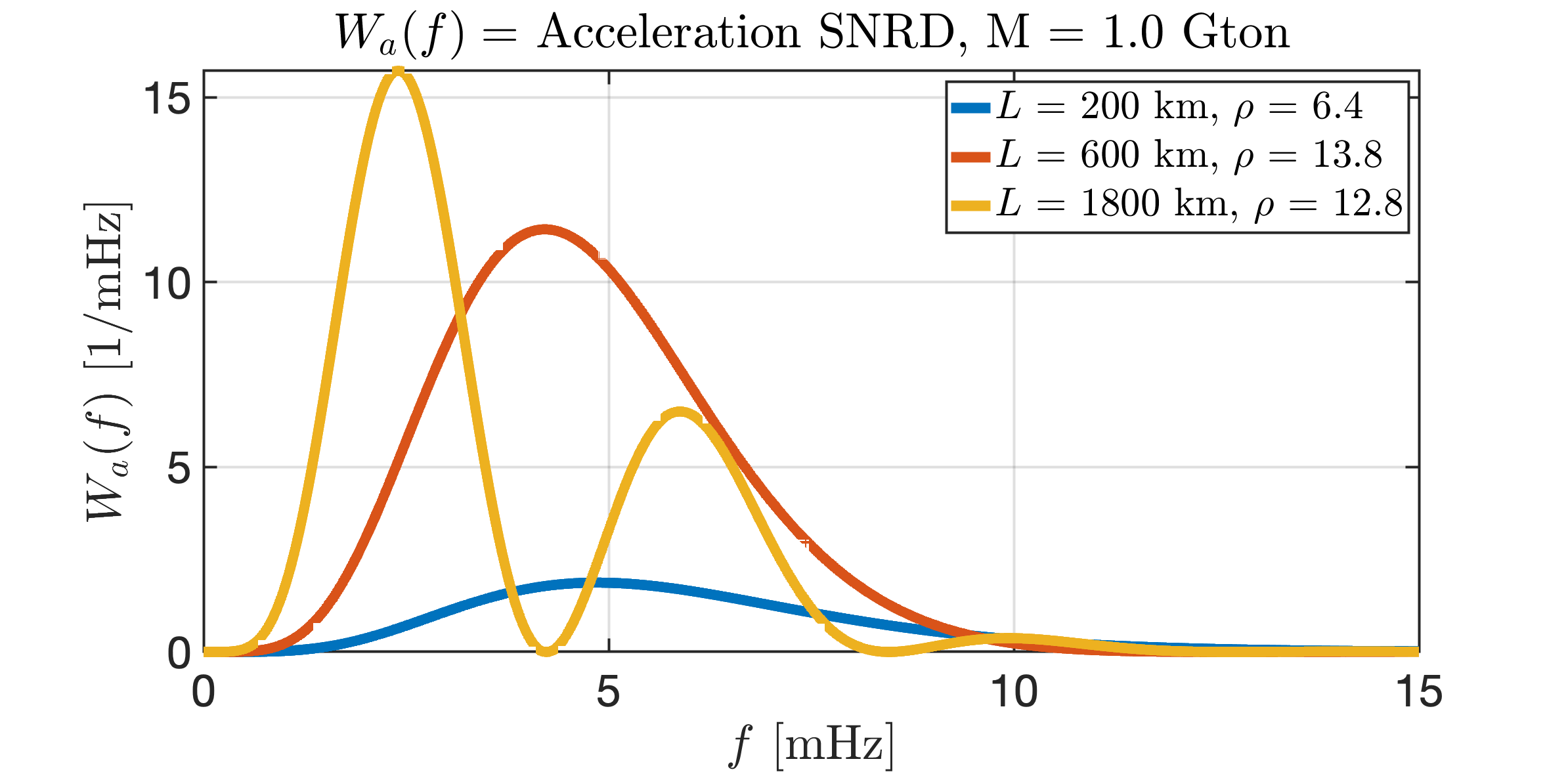
As in Section 2, define the SNRD for range acceleration

W^{\prime}_{a}(f)=\frac{|a_{R}(f)|^{2}/M^{2}}{S_{a}(f)}.

(16)

$W_{a}(f)=W_{a}^{\prime}M^{2}$ is shown in Figure 5 for several values of $L.$ The oscillations with nulls at multiples of $1/\tau=v_{o}/L$ degrade $\rho$ for $L$ beyond an optimum spacecraft separation.

The optimal signal-to-noise ratio per unit mass is

\rho^{\prime}=\sqrt{4\int_{0}^{\infty}W_{a}^{\prime}(f)df},\

(17)

and the source mass that gives $\rho=3$ is (cf. Equation 5)

M_{3}=\frac{3}{\sqrt{4\int_{0}^{\infty}W^{\prime}_{a}(f)df}}.

(18)

From Equations 11 through 16 and Equation 18, the GRACE-FO parameters with the microwave ranging instrument (MWI) and LRI give respectively $M_{3}={\text{\unboldmath$\mathrm{1{.}3}$}}\,\text{\unboldmath$\mathrm{Gt}$},{\text{\unboldmath$\mathrm{0{.}5}$}}\,\text{\unboldmath$\mathrm{Gt}$}.$ The corresponding detectable peak accelerations, $\kappa_{R}M_{3},$ are $\mathrm{0{.}13}$ $\mathrm{nm/s^{2}}$ , $\mathrm{0{.}047}$ $\mathrm{nm/s^{2}}$ .

Another assessment of mass sensitivity for SST laser ranging is inferred from Colombo and Chao, 1992, who proposed a laser ranging mission that, with $(h,L)=(600,\ 500)\,$ km was found by simulation to have sensitivity to weekly changes of $\mathrm{1}$ $\mathrm{mm}$ water height over a square region 400 km across, or mass sensitivity of $\mathrm{160}$ $\mathrm{Mt}$ . In comparison, we find for the LRI on GRACE-FO at the same $(h,L)$ , $M_{3}={\text{\unboldmath$\mathrm{400}$}}\,\text{\unboldmath$\mathrm{Mt}$}.$ The two measurements have different assumed instrument sensitivity and averaging times (week-to-week vs. single-pass).

Figure 6 shows the mass sensitivity $M_{3}$ as a function of $h$ and $L$ for the LRI ranging instrument with two different levels of accelerometer sensitivity: $\tilde{a}_{0}={\text{\unboldmath$\mathrm{7{}\times{}10^{-11}}$}}\,\text{\unboldmath$\mathrm{}$}$ and $\mathrm{7{}\times{}10^{-13}}$ $\mathrm{m/s^{2}/\sqrt{\text{Hz}}}$ . The lower row of Figure 6 shows the optimum $L$ for a given $h$ and the resulting $M_{3}.$ The optimum $L$ for the LRI on GRACE-FO, operating at $h={\text{\unboldmath$\mathrm{500}$}}\,\text{\unboldmath$\mathrm{km}$}$ , is $L={\text{\unboldmath$\mathrm{900}$}}\,\text{\unboldmath$\mathrm{km}$},$ which would give $M_{3}={\text{\unboldmath$\mathrm{200}$}}\,\text{\unboldmath$\mathrm{Mt}$}.$ That reflects a potential factor of 2.5 improvement over $M_{3}={\text{\unboldmath$\mathrm{500}$}}\,\text{\unboldmath$\mathrm{Mt}$}$ for the nominal satellite separation of $L={\text{\unboldmath$\mathrm{200}$}}\,\text{\unboldmath$\mathrm{km}$}.$ A future mission with the improved $\tilde{a}_{0},$ $h={\text{\unboldmath$\mathrm{500}$}}\,\text{\unboldmath$\mathrm{km}$},$ and optimal satellite separation $L={\text{\unboldmath$\mathrm{900}$}}\,\text{\unboldmath$\mathrm{km}$}$ has $M_{3}={\text{\unboldmath$\mathrm{7}$}}\,\text{\unboldmath$\mathrm{Mt}$}.$

3.4 Optimal filter

The filter that gives maximum signal-to-noise ratio is (Wainstein and Zubakov, 1970, Chapter 3)

G(f)=\frac{a_{R}^{*}(f)}{S_{a}(f)},

(19)

with ^∗ denoting complex conjugation. The filter’s input is the measured range acceleration. $G(f)$ is an example of a filter for extracting a signal of known waveform, in this case the range acceleration resulting from flying over a point mass. Dropping the multiplicative constants, the filter magnitude is

|G(f)|=\frac{\left|fK_{0}\left(\frac{2\pi f}{f_{h}}\right)\sin\left(\frac{2\pi f}{f_{L}}\right)\right|}{S_{a}(f)}.

(20)

Normalized $|G(f)|$ for the MWI and LRI on GRACE-FO are shown in Figure 7.

Ghobadi-Far et al., 2018 analyzed the GRACE-FO MWI signal in terms of the line-of-sight gravity difference, and applied the same analysis method to the GRACE-FO LRI signal in Ghobadi-Far et al., 2020. In their analysis of MWI data, Ghobadi-Far et al., 2018 defined the gravimetric quantity $\delta g^{\text{LOS}}_{12},$ or line-of-sight (LOS) gravity difference, which differs from the range acceleration residual $\delta\ddot{\rho}$ by $\Delta_{0},$ the residual centrifugal acceleration:

\delta g_{12}^{\text{LOS}}=\delta\ddot{\rho}+\Delta_{0}.

(21)

Residuals are relative to a reference field. The admittance $Z(f)$ is defined as the ratio of power spectra,

Z(f)=\frac{S_{\delta\ddot{\rho},\delta g_{12}^{\text{LOS}}}(f)}{S_{\delta\ddot{\rho},\delta\ddot{\rho}}(f)},

(22)

where $S_{\delta\ddot{\rho},\delta\ddot{\rho}}(f)$ is the power spectrum of the MWI range acceleration measurement and $S_{\delta\ddot{\rho},\delta g_{12}^{\text{LOS}}}(f)$ is the cross-power spectrum between the range acceleration and the LOS gravity difference. Keeping the shorthand notation $p(f)={\cal F}[p(t)],\ Z(f)$ is a filter that transforms residual range acceleration $\delta\ddot{\rho}(f)=a_{R}(f)$ to $\delta g_{\text{F}}^{\text{LOS}}(f)$ , an estimate of $\delta g^{\text{LOS}}_{12}(f):$

\delta g^{\text{LOS}}_{\text{F}}(f)=Z(f)\delta\ddot{\rho}(f).

(23)

$Z(f),$ normalized to have a maximum value of 1, is shown as the dashed trace in Figure 7. $Z(f)$ is the optimal filter to apply to MWI range acceleration, based on the measurement data that includes signal from the gravity field. It applies to extracting the best SNR from a residual regional or global field and does not explicitly depend on instrument noise spectra.

In contrast, $G(f)$ is fine-tuned to the problem of detecting the specific waveform of a point mass, in the presence of known measurement noise. Since a point mass generates a field with the highest possible frequency content, the $G(f)$ passband starts higher in frequency than $Z(f).$ The LRI $G(f)$ passband is higher than for the MWI because the LRI measurement has reduced noise at high frequency.

A practical use for the $G(f)$ filter is searching for unknown point-like features, such as underground water storage of 100 km spatial extent. The filter would be applied to range acceleration measurements after subtracting the effect of the known field, including time-varying gravity, and non-gravitational accelerations.

4 Conclusion

We derived the optimum sensitivity of orbiting gravimetric satellites to a point source, that is a single mascon. The signal-to-noise ratio is found as a function of instrument noise and orbital parameters. The signal is converted to frequency space by the Fourier transform, and the signal-to-noise ratio is derived from optimal filtering a signal of known waveform. This analysis differs from the conventional approach of spherical harmonic expansion to characterize the field from an arbitrary mass distribution. Such an expansion requires a very large harmonic order to accurately approximate the field from a point source, as shown in A.

The frequency response of an orbiting gradiometer to a point mass directly under the flight track is approximated by Equation 2 that depends only on the orbital altitude and the magnitude of the point mass. Likewise, for an SST-based measurement of the gravitational field, the range acceleration is approximated by Equation 11 that includes dependency on the average satellite separation. Applying Wiener optimal filter theory, these responses and the noise spectra of the ranging measurement and of accelerometer-based measurement of non-gravitational forces give $\rho,$ the maximum achievable signal-to-noise ratio. The resolvable mass $M_{3}$ is defined as the magnitude of the point mass that gives $\rho=3.$ $M_{3}$ is the ultimate mass sensitivity, and realistic non-point mass distributions that are not directly under the flight track will give larger $M_{3}$ in practice. Nonetheless, $M_{3}$ provides a figure of merit for comparing future missions with different orbits and instrument sensitivities to guide the design of such missions. For SST measurements $M_{3}$ has a minimum value at a calculable satellite separation $L,$ giving the optimum separation for discovering point-like (meaning less than approximately 300 km) features such as subsurface water storage. Equation 20 specifies the optimal filter for such a search. As a caveat, the $M_{3}$ metric and its $L$ optimization does not apply to large-scale gravimetry, such as required by oceanography.

Acknowledgments

The author thanks Kirk McKenzie, Gabriel Ramirez, Pep Sanjuan and David Wiese for useful discussions, and Christopher McCullough for key insights. The contributions of four anonymous reviewers, who suggested improvements that are incorporated in this manuscript, is gratefully acknowledged. This research was carried out at the Jet Propulsion Laboratory, California Institute of Technology, under a contract with the National Aeronautics and Space Administration. ©2020 California Institute of Technology. Government sponsorship acknowledged.

Appendix A Multipole expansion and the Wahr equation for surface density

The gravitational potential is conventionally expressed as the multipole expansion (Kaula, 1966, Kaula, 2013, Chao and Gross, 1987)

	$\displaystyle U(r,\theta,\phi)=$	$\displaystyle\frac{GM_{e}}{a}\sum_{n=0}^{\infty}\sum_{m=0}^{n}\left(\frac{a}{r}\right)^{n+1}\overline{P}_{nm}(\cos\theta)$		(24)
		$\displaystyle\times(\overline{C}_{nm}\cos m\phi+\overline{S}_{nm}\sin m\phi).$

As illustrated in Figure 8 $(r,\theta,\phi)$ = (distance from the center of the Earth, co-latitude, longitude), $(a,M_{e})=$ (Earth radius, Earth mass), and $\overline{P}_{nm}$ is the fully-normalized associated Legendre function. The field is entirely specified by the Stokes coefficients $(\overline{C}_{nm},\overline{S}_{nm}).$

For a known mass distribution $dM=\rho(r^{\prime},\theta^{\prime},\phi^{\prime})dV^{\prime}$ with primes designating the source mass coordinates, $(\overline{C}_{nm},\overline{S}_{nm})$ are evaluated as the volume integral Bettadpur, 2018

\begin{bmatrix}\overline{C}_{nm}\\ \overline{S}_{nm}\end{bmatrix}=\frac{1}{(2n+1)M_{e}}\int_{V^{\prime}}dM\,\left(\frac{r^{\prime}}{a}\right)^{n}\overline{P}_{nm}(\lambda^{\prime})\begin{bmatrix}\cos m\phi^{\prime}\\ \sin m\phi^{\prime}\end{bmatrix},

(25)

where $\lambda^{\prime}=\cos\theta^{\prime}.$ For a point mass at $r^{\prime}=a$

\begin{bmatrix}\overline{C}_{nm}\\ \overline{S}_{nm}\end{bmatrix}=\frac{M}{(2n+1)M_{e}}\overline{P}_{nm}(\lambda^{\prime})\begin{bmatrix}\cos m\phi^{\prime}\\ \sin m\phi^{\prime}\end{bmatrix}.

(26)

A single point mass can be placed at the north pole, $(\theta^{\prime},\phi^{\prime})=(0,0)$ without loss of generality. Then

\begin{bmatrix}\overline{C}_{nm}\\ \overline{S}_{nm}\end{bmatrix}=\frac{M}{(2n+1)M_{e}}\overline{P}_{nm}(1)\begin{bmatrix}1\\ 0\end{bmatrix}.

(27)

The relationship between the fully normalized Legendre function $\overline{P}_{nm}$ and the associated Legendre function $P_{nm}$ is

\overline{P}_{nm}=\sqrt{\frac{(2-\delta_{m0})(2n+1)(n-m)!}{(n+m)!}}P_{nm},

(28)

where $\delta_{mn}$ is the Kronecker delta. Since $P_{nm}(1)=\delta_{m0},\ \overline{P}_{nm}(1)=\delta_{m0}\sqrt{2n+1}.$ For a point mass at the pole Equation 26 reduces to

\begin{bmatrix}\overline{C}_{nm}\\ \overline{S}_{nm}\end{bmatrix}=\frac{M}{M_{e}}\frac{1}{\sqrt{2n+1}}\begin{bmatrix}\delta_{m0}\\ 0\end{bmatrix}.

(29)

The potential from Equations 24 and 29 is independent of $\phi$ and is given by the multipole expansion

U(r,\theta)=\frac{GM}{a}\sum_{n=0}^{\infty}\left(\frac{a}{r}\right)^{n+1}P_{n}(\cos\theta),

(30)

the familiar expansion from electrostatics for the azimuthally symmetric electric field from a point charge (Jackson, 2007) and from gravitational potential theory (Blakely, 1996, Section 6.4.2).

The Wahr equation for surface density from $(\overline{C}_{nm},\overline{S}_{nm})$ (Wahr et al., 1998) is

	$\displaystyle\sigma(\theta^{\prime},\phi^{\prime})=$	$\displaystyle\frac{a\rho_{\text{ave}}}{3}\sum_{n=0}^{\infty}\sum_{m=0}^{n}\overline{P}_{nm}(\cos\theta^{\prime})\frac{2n+1}{1+k_{n}}$
		$\displaystyle\times(\overline{C}_{nm}\cos m\phi^{\prime}+\overline{S}_{nm}\sin m\phi^{\prime}),$		(31)

where $k_{n}=$ Love number.

To study the error of a finite-degree spherical harmonic approximation to a point mass, consider a spherical cap in the limit of small cap size. The spherical cap is centered at coordinates $(\theta^{\prime},\phi^{\prime})$ and its angular radius is $\alpha$ and $\lambda\equiv\cos\alpha.$ As computed by Pollack, 1973, the Stokes coefficients are

\begin{bmatrix}\overline{C}_{nm}\\ \overline{S}_{nm}\end{bmatrix}=-\frac{M}{M_{e}}\frac{P_{n+1}-P_{n-1}}{(2n+1)^{2}(1-\lambda)}\overline{P}_{nm}(\cos\theta^{\prime})\begin{bmatrix}\cos m\phi^{\prime}\\ \sin m\phi^{\prime}\end{bmatrix},

(32)

where we use the shorthand $P_{j}(\lambda)=P_{j}.$ For a spherical cap at the north pole,

\begin{bmatrix}\overline{C}_{nm}\\ \overline{S}_{nm}\end{bmatrix}=-\frac{M}{M_{e}}\frac{P_{n+1}-P_{n-1}}{(2n+1)^{3/2}(1-\lambda)}\begin{bmatrix}\delta_{m0}\\ 0\end{bmatrix}.

(33)

The spherical cap reduces to a point mass in the limit of $\alpha=0,\text{ or }\lambda=1$ ; substituting

$\lim_{\lambda\to 1}\left[P_{n+1}-P_{n-1}\right]=(\lambda-1)(2n+1)$ = into Equation 33 gives Equation 29.

By comparing expressions similar to Equation 24 and Equation A, Dickey et al., 1997 identifies

\hat{\overline{C}}_{nm}+\hat{\overline{S}}_{nm}=\frac{\rho_{\text{ave}}}{3\rho_{w}}\frac{2n+1}{1+k_{n}}(\overline{C}_{nm}+\overline{S}_{nm})

(34)

where $\rho_{w}$ is the density of water as the transformation to convert geoid expansion coefficients $(\overline{C}_{nm},\overline{S}_{nm})$ to mass expansion coefficients $(\hat{\overline{C}}_{nm},\hat{\overline{S}}_{nm})$ , p. 101 their Equation (B5).

At the pole, from Equation A, dropping the $n=0$ term that represents the total potential of the Earth, and neglecting the Earth’s elasticity by setting $k_{n}=0,$

\sigma=\frac{a\rho_{\text{ave}}}{3}\sum_{n=1}^{\infty}\overline{P}_{nm}(1)(2n+1)\overline{C}_{nm}.

(35)

From Equation 33,

$\displaystyle\sigma$	$\displaystyle=$	$\displaystyle-\frac{M}{M_{e}}\frac{a}{1-\lambda}\frac{\rho_{\text{ave}}}{3}$	(36)
		$\displaystyle\times\sum_{n=1}^{\infty}\overline{P}_{nm}(1)\frac{2n+1}{(2n+1)^{3/2}}(P_{n+1}-P_{n-1})$
	$\displaystyle=$	$\displaystyle-\frac{M}{M_{e}}\frac{a}{1-\lambda}\frac{\rho_{\text{ave}}}{3}\sum_{n=1}^{\infty}P_{n+1}-P_{n-1}$
	$\displaystyle=$	$\displaystyle\frac{M}{M_{e}}\frac{a\rho_{\text{ave}}}{3}T_{\infty}.$

The quantity $T_{\infty}$ is the $N=\infty$ limit of the truncated sum, defined as

$\displaystyle T_{N}(\lambda)$	$\displaystyle=$	$\displaystyle\frac{1}{1-\lambda}\sum_{n=1}^{N}P_{n-1}-P_{n+1}$	(37)
	$\displaystyle=$	$\displaystyle\frac{1}{1-\lambda}\left(P_{0}+P_{1}-(P_{N}+P_{N+1}\right)$
	$\displaystyle=$	$\displaystyle\frac{1+\lambda-(P_{N}+P_{N+1})}{1-\lambda}.$

For a small spherical cap, $\alpha<<1$ (and $\lambda=\cos\alpha$ slightly $<1$ ), the cap area is $A=\pi(a\alpha)^{2}.$ Using $\sigma=M/A\text{ and }\rho_{\text{ave}}=3M_{e}/(4\pi a^{3}),$ Equation 36 is equivalent to

\frac{\alpha^{2}T_{\infty}(\cos\alpha)}{4}-1=0.

(38)

The fractional error in $\sigma$ due to truncation of the summation Equation 36 at order $N$ is

\epsilon_{N}=\frac{\alpha^{2}T_{N}(\cos\alpha)}{4}-1\approx-P_{N}(\cos\alpha).

(39)

See Figure 9 for $\epsilon_{N}$ with small spherical caps of two different sizes. The slow reduction of $|\epsilon_{N}|$ with increasing $N$ shows that the unfiltered spherical harmonic expansion is ill-suited to characterize the field from a point-like source. The truncation error is often reduced by applying a spectral localizing filter (Panet et al., 2013, Appendix 2); see also Wahr et al., 1998, Swenson and Wahr, 2002, Seo et al., 2005, and Werth et al., 2009.

References

Abich et al., (2019) Abich, K., Abramovici, A., Amparan, B., Baatzsch, A., Bachman Okihiro, B. B., Barr, D. C., Bize, M. P., Bogan, C., Braxmaier, C., Burke, M. J., et al. (2019). In-orbit performance of the GRACE Follow-on laser ranging interferometer. Physical Review Letters, 123(3):031101.
Abramowitz and Stegun, (1964) Abramowitz, M. and Stegun, I. A. (1964). Handbook of Mathematical Functions with Formulas, Graphs, and Mathematical Tables. Dover, New York, ninth Dover printing, tenth GPO printing edition.
Bettadpur, (2018) Bettadpur, S. (2018). GRACE L-2 Product User Manual. Center for Space Research, The University of Texas at Austin. GRACE 327-734, CSR-GR-03-01.
Blakely, (1996) Blakely, Richard J. (1996). Potential Theory in Gravity and Magnetic Applications. Cambridge University Press.
Chao and Gross, (1987) Chao, B. F. and Gross, R. S. (1987). Changes in the Earth’s rotation and low-degree gravitational field induced by earthquakes. Geophysical Journal International, 91(3):569–596.
Christophe et al., (2010) Christophe, B., Marque, J., and Foulon, B. (2010). In-orbit data verification of the accelerometers of the ESA GOCE mission. In SF2A-2010: Proceedings of the Annual meeting of the French Society of Astronomy and Astrophysics, volume 1, page 113.
Colombo and Chao, (1992) Colombo, O. and Chao, B. (1992). Global gravitational change from space in 2001. In IAG Symp., 112, 71–74.
Conklin and Nguyen, (2017) Conklin, J. and Nguyen, A. N. (2017). Drag-free control and drag force recovery of small satellites. In 31st Annual AIAA/USU Conference on Small Satellites.
Dickey et al., (1997) Dickey, J., Bentley, C. R., Bilham, R., Carton, J., Eanes, R., Herring, T. A., Kaula, W., Lagerleof, G., Rojstaczer, S., Smith, W., et al. (1997). Satellite gravity and the geosphere. National Research Council Report, 112.
Drinkwater et al., (2006) Drinkwater, M. R., Haagmans, R., Muzi, D., Popescu, A., Floberghagen, R., Kern, M., and Fehringer, M. (2006). The GOCE gravity mission: ESA’s first core Earth explorer. In Proceedings of the 3rd international GOCE user workshop, pages 6–8.
Flanagan and Hughes, (1998) Flanagan, E. E. and Hughes, S. A. (1998). Measuring gravitational waves from binary black hole coalescences. i. signal to noise for inspiral, merger, and ringdown. Phys. Rev. D, 57:4535–4565.
Ghobadi-Far et al., (2018) Ghobadi-Far, K., Han, S.-C., Weller, S., Loomis, B. D., Luthcke, S. B., Mayer-Gürr, T., and Behzadpour, S. (2018). A transfer function between line-of-sight gravity difference and GRACE intersatellite ranging data and an application to hydrological surface mass variation. Journal of Geophysical Research: Solid Earth, 123(10):9186–9201.
Ghobadi-Far et al., (2020) Ghobadi-Far,K. Han, S.-C., McCullough, C. M. Wiese, D. N., Yuan, D. Landerer, F. W. Sauber, J, Watkins, M. M., (2020) GRACE Follow-On Laser Ranging Interferometer Measurements Uniquely Distinguish Short-Wavelength Gravitational Perturbations. Geophysical Research Letters, 47(16):e2020GL089445.
Han, (2013) Han, S.-C. (2013). Determination and localized analysis of intersatellite line of sight gravity difference: Results from the GRAIL primary mission. Journal of Geophysical Research: Planets, 118(11):2323–2337.
Hauk and Wiese, (2020) Hauk, M. and Wiese, D. N., (2020). New Methods for Linking Science Objectives to Remote Sensing Observations: A Concept Study Using Single-and Dual-Pair Satellite Gravimetry Architectures. Earth and Space Science, 7(3):e2019EA000922.
Jackson, (2007) Jackson, J. D. (2007). Classical electrodynamics. John Wiley & Sons.
Kaula, (1966) Kaula, W. M. (1966). Tests and combination of satellite determinations of the gravity field with gravimetry. Journal of Geophysical Research, 71(22):5303–5314.
Kaula, (2013) Kaula, W. M. (2013). Theory of satellite geodesy: applications of satellites to geodesy. Courier Corporation.
Konopliv et al., (2013) Konopliv, A. S., Park, R. S., Yuan, D.-N., Asmar, S. W., Watkins, M. M., Williams, J. G., Fahnestock, E., Kruizinga, G., Paik, M., Strekalov, D., et al. (2013). The JPL lunar gravity field to spherical harmonic degree 660 from the GRAIL primary mission. Journal of Geophysical Research: Planets, 118(7):1415–1434.
Landerer et al., (2020) Landerer, F., Flechtner, F., Save, H., Webb, F., Bandikova, T., and Bertiger, WI, et al. (2020). Extending the global mass change data record: GRACE follow-on instrument and science data performance. Geophysical Research Letters, 47(12).
McCullough, (2019) McCullough, C., Harvey, N., Save, H., Bandikova, T (2019). Description of Calibrated GRACE-FO Accelerometer Data Products (ACT) GRACE-FO Level-1 Product Version 04 Manual JPL D-103863
Müller, (2017) Müller, V. (2017). Design considerations for future geodesy missions and for space laser interferometry Ph.D. Thesis, Gottfried Wilhelm Leibniz Universität Hannover, 2017.
Numata et al., (2004) Numata, K., Kemery, A., and Camp, J. (2004). Thermal-noise limit in the frequency stabilization of lasers with rigid cavities. Physical Review Letters, 93(25):250602.
Panet et al., (2013) Panet, I., Flury, J., Biancale, R., Gruber, T., Johannessen, J., van den Broeke, M., van Dam, T., Gegout, P., Hughes, C., Ramillien, G., et al. (2013). Earth system mass transport mission (e. motion): a concept for future Earth gravity field measurements from space. Surveys in Geophysics, 34(2):141–163.
Pollack, (1973) Pollack, H. N. (1973). Spherical harmonic representation of the gravitational potential of a point mass, a spherical cap, and a spherical rectangle. Journal of Geophysical Research, 78(11):1760–1768.
Reigber et al., (2003) Reigber, C., Schwintzer, P., Neumayer, K.-H., Barthelmes, F., König, R., Förste, C., Balmino, G., Biancale, R., Lemoine, J.-M., Loyer, S., et al. (2003). The CHAMP-only Earth gravity field model EIGEN-2. Advances in Space Research, 31(8):1883–1888.
Seo et al., (2005) Seo, K.-W., Wilson, C., Chen, J., Famiglietti, J., and Rodell, M. (2005). Filters to estimate water storage variations from GRACE. In IAG Symp., 128, 607–611. Springer.
Swenson and Wahr, (2002) Swenson, S. and Wahr, J. (2002). Methods for inferring regional surface-mass anomalies from gravity recovery and climate experiment (GRACE) measurements of time-variable gravity. Journal of Geophysical Research: Solid Earth, 107(B9):ETG–3.
Tapley, (1997) Tapley, B. D (1997). Evaluation of Flat-Earth Approximation Results for Geopotential Missions. Journal of Guidance, Control, and Dynamics, 20(2):246–252.
Tapley et al., (2004) Tapley, B. D., Bettadpur, S., Ries, J. C., Thompson, P. F., and Watkins, M. M. (2004). GRACE measurements of mass variability in the Earth system. Science, 305(5683):503–505.
Touboul et al., (1999) Touboul, P., Willemenot, E., Foulon, B., and Josselin, V. (1999). Accelerometers for CHAMP, GRACE and GOCE space missions: synergy and evolution. Boll. Geof. Teor. Appl, 40(3-4):321–327.
(32) Touboul, P., Foulon, B., and Willemenot (1999a). Electrostatic space accelerometers for present and future missions. Acta Astronautica, 45(10):605–617.
Wahr et al., (1998) Wahr, J., Molenaar, M., and Bryan, F. (1998). Time variability of the Earth’s gravity field: Hydrological and oceanic effects and their possible detection using GRACE. Journal of Geophysical Research: Solid Earth, 103(B12):30205–30229.
Wainstein and Zubakov, (1970) Wainstein, L. A. and Zubakov, V. (1970). Extraction of signals from noise. PrenticeHall, Englewood Cliffs, NJ.
Watkins et al., (2015) Watkins, M., Wiese, D. N., Yuan, D.-N., Boening, C., and Landerer, F. W. (2015). Improved methods for observing Earth’s time variable mass distribution with GRACE using spherical cap mascons. Journal of Geophysical Research: Solid Earth, 120(4):2648–2671.
Watkins et al., (2005) Watkins, M., Yuan, D., Kuang, D., Bertiger, W., Kim, M., and Kruizinga, G. (2005). GRACE harmonic and mascon solutions at JPL. AGU Fall Meeting, 2005:G22A–04.
Werth et al., (2009) Werth, S., Güntner, A., Schmidt, R., and Kusche, J. (2009). Evaluation of GRACE filter tools from a hydrological perspective. Geophysical Journal International, 179(3):1499–1515.
Wolff, (1969) Wolff, M. (1969). Direct measurements of the Earth’s gravitational potential using a satellite pair. Journal of Geophysical Research, 74(22):5295–5300.
Wong et al., (1971) Wong, L., Buechler, G., Downs, W., Sjogren, W., Muller, P., and Gottlieb, P. (1971). A surface-layer representation of the lunar gravitational field. Journal of Geophysical Research, 76(26):6220–6236.