Masses of doubly heavy tetraquarks $T_{QQ^{\prime}}$ in a relativized quark model

Qi-Fang Lü Email: lvqifang@hunnu.edu.cn Affiliation: Department of Physics, Hunan Normal University, Changsha 410081, China Affiliation: Synergetic Innovation Center for Quantum Effects and Applications (SICQEA), Changsha 410081,China Affiliation: Key Laboratory of Low-Dimensional Quantum Structures and Quantum Control of Ministry of Education, Changsha 410081, China Dian-Yong Chen Email: chendy@seu.edu.cn Affiliation: School of Physics, Southeast University, Nanjing 210094, China Yu-Bing Dong Email: dongyb@ihep.ac.cn Affiliation: Institute of High Energy Physics, Chinese Academy of Sciences, Beijing 100049, China Affiliation: Theoretical Physics Center for Science Facilities (TPCSF), CAS, Beijing 100049, China Affiliation: School of Physical Sciences, University of Chinese Academy of Sciences, Beijing 101408, China

Abstract

In the present work, the mass spectra of doubly heavy tetraquarks $T_{QQ^{\prime}}$ are systematically investigated in a relativized quark model. The four-body systems including the Coulomb potential, confining potential, spin-spin interactions, and relativistic corrections are solved within the variational method. Our results suggest that the $IJ^{P}=01^{+}$ $bb\bar{u}\bar{d}$ state is 54 MeV below the relevant $\bar{B}\bar{B}$ and $\bar{B}\bar{B}^{*}$ thresholds, which indicates that both strong and electromagnetic decays are forbidden, and thus this state can be a stable one. Its large hidden color component and small root mean square radius demonstrate that it is a compact tetraquark rather than a loosely bound molecule or point-like diquark-antidiquark structure. Our predictions of the doubly heavy tetraquarks may provide valuable information for future experimental searches.

I Introduction

In the past two decades, plenty of new resonances have been observed in the hadronic physics, and some of them can be hardly classified into the conventional hadron sectors, i.e., mesons and baryons Tanabashi:2018oca. These exotic structures have attracted extensive theoretical and experimental interests due to their enigmatic properties Chen:2016qju; Hosaka:2016pey; Richard:2016eis; Lebed:2016hpi; Ali:2017jda; Esposito:2016noz; Guo:2017jvc; Olsen:2017bmm; Karliner:2017qhf; Liu:2019zoy; Brambilla:2019esw. To describe their inner structures, new effective degree of freedom are introduced to go beyond the traditional quark-antiquark and three-quark configurations. The experimental observations of charged quarkonium-like states $Z_{c(b)}$ Choi:2007wga; Aaij:2014jqa; Belle:2011aa; Ablikim:2013mio; Liu:2013dau and pentaquark states $P_{c}$ Aaij:2015tga; Aaij:2019vzc provide strong evidences for the existence of the exotic hadrons in QCD. Besides these hidden charm and bottom ones, it is also expected that the open flavor exotic states should exist. However, the experimental searches for these flavored exotic hadrons were beset with difficulties and obstacles, and the experiences of failures, such as $\Theta^{+}(1540)$ Nakano:2003qx and $X(5568)$ D0:2016mwd; Aaij:2016iev, have casted a shadow over this research area.

The situation began to change in 2017, when a doubly heavy baryon $\Xi_{cc}^{++}$ was observed by the LHCb Collaboration Aaij:2017ueg. Although the $\Xi_{cc}^{++}$ is regarded as a $S-$ wave conventional baryon, it provides an excellent opportunity to examine the interactions between two heavy quarks and search for more doubly heavy quark systems. Indeed, based on the mass of $\Xi_{cc}^{++}$ , the mass spectra of doubly heavy tetraquark states $T_{QQ^{\prime}}$ were studied subsequently, which indicate that there should exist at least one stable flavored exotic tetraquark $bb\bar{u}\bar{d}$ Karliner:2017qjm; Eichten:2017ffp.

Actually, the doubly heavy tetraquarks $T_{QQ^{\prime}}$ have been discussed for a long time. Before the observation of $\Xi_{cc}^{++}$ , there have been a number of theoretical works on the doubly heavy tetraquarks. Various approaches, involving quark models Karliner:2017qjm; Eichten:2017ffp; Ballot:1983iv; Lipkin:1986dw; Vijande:2009ac; Luo:2017eub; Ebert:2007rn; Semay:1994ht; Zouzou:1986qh; Heller:1986bt; Carlson:1987hh; SilvestreBrac:1993ss; SilvestreBrac:1993ry; Pepin:1996id; Brink:1998as; Vijande:2003ki; Zhang:2007mu; Vijande:2009kj; Yang:2009zzp, QCD sum rules Navarra:2007yw; Dias:2011mi; Chen:2013aba; Du:2012wp, and lattice QCD Ikeda:2013vwa; Bicudo:2015kna; Francis:2016hui; Bicudo:2017szl, were adopted to estimate their mass spectra. Due to the lack of experimental information on the doubly heavy systems, it is difficult to distinguish those numerous results. Also, several works have investigated their production mechanism, which should be helpful for experimental searches Gelman:2002wf; Janc:2004qn; DelFabbro:2004ta; Yuqi:2011gm; Hyodo:2012pm. Lately, stimulated by the observation of $\Xi_{cc}^{++}$ , the studies on doubly heavy systems were revived and have interested plenty of theorists and experimenters. In particular, the properties for the doubly heavy tetraquarks, such as their masses, decays, and production rates, have been extensively discussed in the past years Mehen:2017nrh; Wang:2017dtg; Yan:2018gik; Ali:2018ifm; Xing:2018bqt; Agaev:2018vag; Ali:2018xfq; Park:2018wjk; Agaev:2018khe; Francis:2018jyb; Junnarkar:2018twb; Deng:2018kly; Caramees:2018oue; Agaev:2019qqn; Sundu:2019feu; Maiani:2019cwl; Zhu:2019iwm; Maiani:2019lpu; Fontoura:2019opw; Agaev:2019kkz; Leskovec:2019ioa; Liu:2019yye; Hernandez:2019eox; Yang:2019itm; Tang:2019nwv; Agaev:2020dba; Wang:2020jgb; Tan:2020ldi. Within different frameworks, these studies present distinctive results and conclusions. However, almost all the works agree that the isoscalar $T_{bb}$ state should be stable against its strong and electromagnetic decays. The binding energy relative to the $\bar{B}\bar{B}^{*}$ threshold is predicted to be more than 100 MeV by most studies, which is deeply bound and leads to a compact configuration.

Within the framework of quark models, the previous studies were mainly based on the nonrelativistic quark potential models or simple quark models. Since the doubly heavy tetraquarks also include two light antiquarks, the relativistic corrections for the mass spectra may be significant. For instance, the masses of doubly heavy tetraquarks are calculated within a relativistic quark model under the diquark approximation Ebert:2007rn. However, the four-body calculations together with relativistic effects have not been done in the literature. Therefore, before making a final conclusion on the isoscalar $T_{bb}$ state, it is essential to perform a calculation in a relativized quark model with few-body method for the doubly heavy tetraquark spectra.

In this issue, we investigate the mass spectra of doubly heavy tetraquarks $T_{QQ^{\prime}}$ in the relativized quark model proposed by Godfrey, Capstick, and Isgur Godfrey:1985xj; Capstick:1986bm. This model has been extensively adopted to study the properties of conventional hadrons and it may give a unified description of different flavor sectors. Also, under the diquark approximation, the authors have employed the relativized quark model to deal with the tetraquark states and achieved satisfactory results Lu:2016cwr; Lu:2016zhe; Lu:2019ira; Anwar:2017toa; Anwar:2018sol; Bedolla:2019zwg; Ferretti:2020ewe. Thus, the relativized quark model is suitable for us to deal with the doubly heavy tetraquarks, where all the heavy-heavy, heavy-light, and light-light quark interactions are involved. For the first time, we extend the relativized quark model to investigate the double heavy tetraquark spectra by solving a four-body Schrödinger-type equation. With the present extension, the tetraquark, as well as the conventional hadrons can be described in a uniform frame.

This paper is organized as follows. The framework of relativized quark model and few-body method are introduced in Sec. II. The results and discussions of doubly heavy tetraquark spectra are given in Sec. III. A summary is presented in the last section.

II Model

II.1 Hamiltonian

To calculate the mass spectra of doubly heavy tetraquarks $T_{QQ^{\prime}}\equiv QQ^{\prime}\bar{q}\bar{q}^{\prime}$ , the relativized Hamiltonian should be constructed. Similar to the procedures of the conventional mesons and baryons Godfrey:1985xj; Capstick:1986bm, the relativized Hamiltonian for a $QQ^{\prime}\bar{q}\bar{q}^{\prime}$ tetraquark state can be written as

H=H_{0}+\sum_{i<j}V_{ij}^{\rm oge}+\sum_{i<j}V_{ij}^{\rm conf},

(1)

where $H_{0}$ is a relativistic kinetic energy term

H_{0}=\sum_{i=1}^{4}(p_{i}^{2}+m_{i}^{2})^{1/2}.

(2)

The $V_{ij}^{\rm oge}$ is the one gluon exchange pairwise potential, and $V_{ij}^{\rm conf}$ corresponds to the confining part. The kinematic energy of the center-of-mass system can be eliminated by the constraint $\sum_{i=1}^{4}\bm{p}_{i}=0$ .

In present work, we only concentrate on the $S-$ wave ground states and do not include the spin-orbit and tensor interactions. Then, the potential $V_{ij}^{\rm oge}$ can be expressed as

V_{ij}^{\rm{oge}}=\beta_{ij}^{1/2}\tilde{G}(r_{ij})\beta_{ij}^{1/2}+\delta_{ij}^{1/2+\epsilon_{c}}\frac{2\bm{S_{i}}\cdot\bm{S_{j}}}{3m_{i}m_{j}}\nabla^{2}\tilde{G}(r_{ij})\delta_{ij}^{1/2+\epsilon_{c}},

(3)

with

\beta_{ij}=1+\frac{p_{ij}^{2}}{(p_{ij}^{2}+m_{i}^{2})^{1/2}(p_{ij}^{2}+m_{j}^{2})^{1/2}},

(4)

and

\delta_{ij}=\frac{m_{i}m_{j}}{(p_{ij}^{2}+m_{i}^{2})^{1/2}(p_{ij}^{2}+m_{j}^{2})^{1/2}}.

(5)

The $p_{ij}$ is the magnitude of the momentum of either of the quarks in the center-of-mass frame of $ij$ quark subsystem, and the $\epsilon_{c}$ is a free parameter reflecting the momentum dependence. The smeared Coulomb potential $\tilde{G}(r_{ij})$ is

\tilde{G}(r_{ij})=\bm{F}_{i}\cdot\bm{F}_{j}\sum_{k=1}^{3}\frac{\alpha_{k}}{r_{ij}}{\rm erf}(\tau_{kij}r_{ij}),

(6)

with

\frac{1}{\tau_{kij}^{2}}=\frac{1}{\gamma_{k}^{2}}+\frac{1}{\sigma_{ij}^{2}},

(7)

and

\sigma_{ij}^{2}=\sigma_{0}^{2}\left[\frac{1}{2}+\frac{1}{2}\left(\frac{4m_{i}m_{j}}{(m_{i}+m_{j})^{2}}\right)^{4}\right]+s^{2}\left(\frac{2m_{i}m_{j}}{m_{i}+m_{j}}\right)^{2}.

(8)

The $\bm{F}_{i}\cdot\bm{F}_{j}$ stands for the color matrix and reads

\bm{F}_{i}=\left\{\begin{aligned} &\frac{\lambda_{i}}{2}~~~{\rm for~quarks,}\\ &-\frac{\lambda_{i}^{*}}{2}~{\rm for~antiquarks.}\\ \end{aligned}\right.

(9)

Similarly, the confining interaction $V_{ij}^{\rm conf}$ can be expressed as

V_{ij}^{\rm{conf}}=-\frac{3}{4}\bm{F}_{i}\cdot\bm{F}_{j}\left\{br\left[\frac{e^{-\sigma_{ij}^{2}r^{2}}}{\sqrt{\pi}\sigma_{ij}r}+\left(1+\frac{1}{2\sigma_{ij}^{2}r^{2}}\right){\rm erf}(\sigma_{ij}r)\right]+c\right\}.

(10)

All the parameters used here are taken from the original reference Godfrey:1985xj and collected in Table 1 for convenience. The details of the relativized procedure can be found in Refs. Godfrey:1985xj; Capstick:1986bm.

Table 1: Relevant parameters of the relativized quark model Godfrey:1985xj.

$m_{u}/m_{d}(\rm MeV)$	$m_{s}(\rm MeV)$	$m_{c}(\rm MeV)$	$m_{b}(\rm MeV)$	$\alpha_{1}$
220	419	1628	4977	0.25
$\alpha_{2}$	$\alpha_{3}$	$\gamma_{1}(\rm GeV)$	$\gamma_{2}(\rm GeV)$	$\gamma_{3}(\rm GeV)$
0.15	0.20	1/2	$\sqrt{10}/2$	$\sqrt{1000}/2$
$b(\rm GeV^{2})$	$c(\rm MeV)$	$\sigma_{0}(\rm GeV)$	$s$	$\epsilon_{c}$
0.18	-253	1.80	1.55	-0.168

II.2 Matrix elements of color, flavor, and spin parts

The wave function of a $Q_{1}Q_{2}^{\prime}\bar{q}_{3}\bar{q}_{4}^{\prime}$ state can be divided into color, flavor, spin, and spatial parts. In the color space, one has two kinds of colorless states with well defined permutation properties,

|\bar{3}3\rangle=|(Q_{1}Q_{2}^{\prime})^{\bar{3}}(\bar{q}_{3}\bar{q}_{4}^{\prime})^{3}\rangle,

(11)

|6\bar{6}\rangle=|(Q_{1}Q_{2}^{\prime})^{6}(\bar{q}_{3}\bar{q}_{4}^{\prime})^{\bar{6}}\rangle,

(12)

where the $|\bar{3}3\rangle$ is antisymmetric under the exchange of both quarks and antiquarks, and the $|6\bar{6}\rangle$ is the symmetric one. One can evaluate the color matrix elements $\langle\bm{F}_{i}\cdot\bm{F}_{j}\rangle$ with the help of explicit color wave functions or the SU(3) Casimir operator. The results are collected in Table 2.

Table 2: Color matrix elements.

$\langle\hat{O}\rangle$	$\langle\bm{F}_{1}\cdot\bm{F}_{2}\rangle$	$\langle\bm{F}_{3}\cdot\bm{F}_{4}\rangle$	$\langle\bm{F}_{1}\cdot\bm{F}_{3}\rangle$	$\langle\bm{F}_{2}\cdot\bm{F}_{4}\rangle$	$\langle\bm{F}_{1}\cdot\bm{F}_{4}\rangle$	$\langle\bm{F}_{2}\cdot\bm{F}_{3}\rangle$
$\langle\bar{3}3\|\hat{O}\|\bar{3}3\rangle$	-2/3	-2/3	-1/3	-1/3	-1/3	-1/3
$\langle 6\bar{6}\|\hat{O}\|6\bar{6}\rangle$	1/3	1/3	-5/6	-5/6	-5/6	-5/6
$\langle\bar{3}3\|\hat{O}\|6\bar{6}\rangle$	0	0	$-1/\sqrt{2}$	$-1/\sqrt{2}$	$1/\sqrt{2}$	$1/\sqrt{2}$

For the flavor part, the combination between quarks $\bar{u}$ and $\bar{d}$ can be symmetric with $I=1$ or antisymmetric with $I=0$ , while the combinations of $\bar{s}\bar{s}$ , $cc$ , and $bb$ are always symmetric. For combinations $\bar{u}\bar{s}$ and $\bar{d}\bar{s}$ , one can also construct the symmetric and antisymmetric flavor wave functions under the flavor SU(3) symmetry. The $c$ and $b$ are treated as different particles and no symmetry constraint should be obeyed. For convenience, the notation $\bar{u}\bar{d}$ represents the combinations of $\bar{u}\bar{u}$ , $\bar{d}\bar{d}$ , $(\bar{u}\bar{d}+\bar{d}\bar{u})/\sqrt{2}$ , and $(\bar{u}\bar{d}-\bar{d}\bar{u})/\sqrt{2}$ , and notation $\bar{u}\bar{s}$ stands for the combinations $(\bar{u}\bar{s}+\bar{s}\bar{u})/\sqrt{2}$ , $(\bar{u}\bar{s}-\bar{s}\bar{u})/\sqrt{2}$ , $(\bar{d}\bar{s}+\bar{s}\bar{d})/\sqrt{2}$ , and $(\bar{d}\bar{s}-\bar{s}\bar{d})/\sqrt{2}$ in the present work.

In the spin space, one can construct six spin states,

\chi^{00}_{0}=|(Q_{1}Q_{2}^{\prime})_{0}(\bar{q}_{3}\bar{q}_{4}^{\prime})_{0}\rangle_{0},

(13)

\chi^{11}_{0}=|(Q_{1}Q_{2}^{\prime})_{1}(\bar{q}_{3}\bar{q}_{4}^{\prime})_{1}\rangle_{0},

(14)

\chi^{01}_{1}=|(Q_{1}Q_{2}^{\prime})_{0}(\bar{q}_{3}\bar{q}_{4}^{\prime})_{1}\rangle_{1},

(15)

\chi^{10}_{1}=|(Q_{1}Q_{2}^{\prime})_{1}(\bar{q}_{3}\bar{q}_{4}^{\prime})_{0}\rangle_{1},

(16)

\chi^{11}_{1}=|(Q_{1}Q_{2}^{\prime})_{1}(\bar{q}_{3}\bar{q}_{4}^{\prime})_{1}\rangle_{1},

(17)

\chi^{11}_{2}=|(Q_{1}Q_{2}^{\prime})_{1}(\bar{q}_{3}\bar{q}_{4}^{\prime})_{1}\rangle_{2},

(18)

where $(Q_{1}Q_{2}^{\prime})_{0}$ and $(\bar{q}_{3}\bar{q}_{4}^{\prime})_{0}$ are antisymmetric for the two fermions under permutations, and the $(Q_{1}Q_{2}^{\prime})_{1}$ and $(\bar{q}_{3}\bar{q}_{4}^{\prime})_{1}$ are symmetric. For the notation $\chi^{S_{12}S_{34}}_{S}$ , the $S_{12}$ , $S_{34}$ , and $S$ are the spin of two heavy quarks, spin of two light antiquarks, and total spin, respectively. The relevant spin matrix elements can be evaluated with the standard angular momentum algebra, and the results are listed in Table 3.

Table 3: Spin matrix elements.

$\langle\hat{O}\rangle$	$\langle\bm{S}_{1}\cdot\bm{S}_{2}\rangle$	$\langle\bm{S}_{3}\cdot\bm{S}_{4}\rangle$	$\langle\bm{S}_{1}\cdot\bm{S}_{3}\rangle$	$\langle\bm{S}_{2}\cdot\bm{S}_{4}\rangle$	$\langle\bm{S}_{1}\cdot\bm{S}_{4}\rangle$	$\langle\bm{S}_{2}\cdot\bm{S}_{3}\rangle$
$\langle\chi^{00}_{0}\|\hat{O}\|\chi^{00}_{0}\rangle$	-3/4	-3/4	0	0	0	0
$\langle\chi^{11}_{0}\|\hat{O}\|\chi^{11}_{0}\rangle$	1/4	1/4	-1/2	-1/2	-1/2	-1/2
$\langle\chi^{00}_{0}\|\hat{O}\|\chi^{11}_{0}\rangle$	0	0	$-\sqrt{3}/4$	$-\sqrt{3}/4$	$\sqrt{3}/4$	$\sqrt{3}/4$
$\langle\chi^{01}_{1}\|\hat{O}\|\chi^{01}_{1}\rangle$	-3/4	1/4	0	0	0	0
$\langle\chi^{10}_{1}\|\hat{O}\|\chi^{10}_{1}\rangle$	1/4	-3/4	0	0	0	0
$\langle\chi^{11}_{1}\|\hat{O}\|\chi^{11}_{1}\rangle$	1/4	1/4	-1/4	-1/4	-1/4	-1/4
$\langle\chi^{01}_{1}\|\hat{O}\|\chi^{10}_{1}\rangle$	0	0	1/4	1/4	-1/4	-1/4
$\langle\chi^{01}_{1}\|\hat{O}\|\chi^{11}_{1}\rangle$	0	0	$-\sqrt{2}/4$	$\sqrt{2}/4$	$-\sqrt{2}/4$	$\sqrt{2}/4$
$\langle\chi^{10}_{1}\|\hat{O}\|\chi^{11}_{1}\rangle$	0	0	$\sqrt{2}/4$	$-\sqrt{2}/4$	$-\sqrt{2}/4$	$\sqrt{2}/4$
$\langle\chi^{11}_{2}\|\hat{O}\|\chi^{11}_{2}\rangle$	1/4	1/4	1/4	1/4	1/4	1/4

For a $S-$ wave $T_{QQ^{\prime}}$ state, the spatial part is always symmetric, and then the color-spin-flavor wave function should be antisymmetric for the identical quarks and antiquarks according to the Pauli exclusion principle. From the above discussions, we perform all possible configurations for the $QQ^{\prime}\bar{q}\bar{q}^{\prime}$ systems in Table 4. It should be noted that for a given system different configurations with same isospin-spin can mix with each other.

Table 4: All possible configurations for the

QQ^{\prime}\bar{q}\bar{q}^{\prime}

systems. The subscripts and superscripts are the spin quantum numbers and color types, respectively. The braces

\{~\}

, brackets

[~]

strand for the symmetric, antisymmetric flavor wave functions, respectively. The parentheses

(~)

are used for the subsystems without permutation symmetries.

System	$IJ^{P}$	Configuration
$\{cc\}[\bar{u}\bar{d}]$	$01^{+}$	$\|\{cc\}^{\bar{3}}_{1}[\bar{u}\bar{d}]^{3}_{0}\rangle_{1}$	$\|\{cc\}^{6}_{0}[\bar{u}\bar{d}]^{\bar{6}}_{1}\rangle_{1}$	$\cdots$
$\{cc\}\{\bar{u}\bar{d}\}$	$10^{+}$	$\|\{cc\}^{\bar{3}}_{1}\{\bar{u}\bar{d}\}^{3}_{1}\rangle_{0}$	$\|\{cc\}^{6}_{0}\{\bar{u}\bar{d}\}^{\bar{6}}_{0}\rangle_{0}$	$\cdots$
	$11^{+}$	$\|\{cc\}^{\bar{3}}_{1}\{\bar{u}\bar{d}\}^{3}_{1}\rangle_{1}$	$\cdots$	$\cdots$
	$12^{+}$	$\|\{cc\}^{\bar{3}}_{1}\{\bar{u}\bar{d}\}^{3}_{1}\rangle_{2}$	$\cdots$	$\cdots$
$\{bb\}[\bar{u}\bar{d}]$	$01^{+}$	$\|\{bb\}^{\bar{3}}_{1}[\bar{u}\bar{d}]^{3}_{0}\rangle_{1}$	$\|\{bb\}^{6}_{0}[\bar{u}\bar{d}]^{\bar{6}}_{1}\rangle_{1}$	$\cdots$
$\{bb\}\{\bar{u}\bar{d}\}$	$10^{+}$	$\|\{bb\}^{\bar{3}}_{1}\{\bar{u}\bar{d}\}^{3}_{1}\rangle_{0}$	$\|\{bb\}^{6}_{0}\{\bar{u}\bar{d}\}^{\bar{6}}_{0}\rangle_{0}$	$\cdots$
	$11^{+}$	$\|\{bb\}^{\bar{3}}_{1}\{\bar{u}\bar{d}\}^{3}_{1}\rangle_{1}$	$\cdots$	$\cdots$
	$12^{+}$	$\|\{bb\}^{\bar{3}}_{1}\{\bar{u}\bar{d}\}^{3}_{1}\rangle_{2}$	$\cdots$	$\cdots$
$(cb)[\bar{u}\bar{d}]$	$00^{+}$	$\|(cb)^{\bar{3}}_{0}[\bar{u}\bar{d}]^{3}_{0}\rangle_{0}$	$\|(cb)^{6}_{1}[\bar{u}\bar{d}]^{\bar{6}}_{1}\rangle_{0}$	$\cdots$
	$01^{+}$	$\|(cb)^{\bar{3}}_{1}[\bar{u}\bar{d}]^{3}_{0}\rangle_{1}$	$\|(cb)^{6}_{0}[\bar{u}\bar{d}]^{\bar{6}}_{1}\rangle_{1}$	$\|(cb)^{6}_{1}[\bar{u}\bar{d}]^{\bar{6}}_{1}\rangle_{1}$
	$02^{+}$	$\|(cb)^{6}_{1}[\bar{u}\bar{d}]^{\bar{6}}_{1}\rangle_{2}$	$\cdots$	$\cdots$
$(cb)\{\bar{u}\bar{d}\}$	$10^{+}$	$\|(cb)^{\bar{3}}_{1}\{\bar{u}\bar{d}\}^{3}_{1}\rangle_{0}$	$\|(cb)^{6}_{0}\{\bar{u}\bar{d}\}^{\bar{6}}_{0}\rangle_{0}$	$\cdots$
	$11^{+}$	$\|(cb)^{\bar{3}}_{0}\{\bar{u}\bar{d}\}^{3}_{1}\rangle_{1}$	$\|(cb)^{\bar{3}}_{1}\{\bar{u}\bar{d}\}^{3}_{1}\rangle_{1}$	$\|(cb)^{6}_{1}\{\bar{u}\bar{d}\}^{\bar{6}}_{0}\rangle_{1}$
	$12^{+}$	$\|(cb)^{\bar{3}}_{1}\{\bar{u}\bar{d}\}^{3}_{1}\rangle_{2}$	$\cdots$	$\cdots$
$\{cc\}[\bar{u}\bar{s}]$	$\frac{1}{2}1^{+}$	$\|\{cc\}^{\bar{3}}_{1}[\bar{u}\bar{s}]^{3}_{0}\rangle_{1}$	$\|\{cc\}^{6}_{0}[\bar{u}\bar{s}]^{\bar{6}}_{1}\rangle_{1}$	$\cdots$
$\{cc\}\{\bar{u}\bar{s}\}$	$\frac{1}{2}0^{+}$	$\|\{cc\}^{\bar{3}}_{1}\{\bar{u}\bar{s}\}^{3}_{1}\rangle_{0}$	$\|\{cc\}^{6}_{0}\{\bar{u}\bar{s}\}^{\bar{6}}_{0}\rangle_{0}$	$\cdots$
	$\frac{1}{2}1^{+}$	$\|\{cc\}^{\bar{3}}_{1}\{\bar{u}\bar{s}\}^{3}_{1}\rangle_{1}$	$\cdots$	$\cdots$
	$\frac{1}{2}2^{+}$	$\|\{cc\}^{\bar{3}}_{1}\{\bar{u}\bar{s}\}^{3}_{1}\rangle_{2}$	$\cdots$	$\cdots$
$\{bb\}[\bar{u}\bar{s}]$	$\frac{1}{2}1^{+}$	$\|\{bb\}^{\bar{3}}_{1}[\bar{u}\bar{s}]^{3}_{0}\rangle_{1}$	$\|\{bb\}^{6}_{0}[\bar{u}\bar{s}]^{\bar{6}}_{1}\rangle_{1}$	$\cdots$
$\{bb\}\{\bar{u}\bar{s}\}$	$\frac{1}{2}0^{+}$	$\|\{bb\}^{\bar{3}}_{1}\{\bar{u}\bar{s}\}^{3}_{1}\rangle_{0}$	$\|\{bb\}^{6}_{0}\{\bar{u}\bar{s}\}^{\bar{6}}_{0}\rangle_{0}$	$\cdots$
	$\frac{1}{2}1^{+}$	$\|\{bb\}^{\bar{3}}_{1}\{\bar{u}\bar{s}\}^{3}_{1}\rangle_{1}$	$\cdots$	$\cdots$
	$\frac{1}{2}2^{+}$	$\|\{bb\}^{\bar{3}}_{1}\{\bar{u}\bar{s}\}^{3}_{1}\rangle_{2}$	$\cdots$	$\cdots$
$(cb)[\bar{u}\bar{s}]$	$\frac{1}{2}0^{+}$	$\|(cb)^{\bar{3}}_{0}[\bar{u}\bar{s}]^{3}_{0}\rangle_{0}$	$\|(cb)^{6}_{1}[\bar{u}\bar{s}]^{\bar{6}}_{1}\rangle_{0}$	$\cdots$
	$\frac{1}{2}1^{+}$	$\|(cb)^{\bar{3}}_{1}[\bar{u}\bar{s}]^{3}_{0}\rangle_{1}$	$\|(cb)^{6}_{0}[\bar{u}\bar{s}]^{\bar{6}}_{1}\rangle_{1}$	$\|(cb)^{6}_{1}[\bar{u}\bar{s}]^{\bar{6}}_{1}\rangle_{1}$
	$\frac{1}{2}2^{+}$	$\|(cb)^{6}_{1}[\bar{u}\bar{s}]^{\bar{6}}_{1}\rangle_{2}$	$\cdots$	$\cdots$
$(cb)\{\bar{u}\bar{s}\}$	$\frac{1}{2}0^{+}$	$\|(cb)^{\bar{3}}_{1}\{\bar{u}\bar{s}\}^{3}_{1}\rangle_{0}$	$\|(cb)^{6}_{0}\{\bar{u}\bar{s}\}^{\bar{6}}_{0}\rangle_{0}$	$\cdots$
	$\frac{1}{2}1^{+}$	$\|(cb)^{\bar{3}}_{0}\{\bar{u}\bar{s}\}^{3}_{1}\rangle_{1}$	$\|(cb)^{\bar{3}}_{1}\{\bar{u}\bar{s}\}^{3}_{1}\rangle_{1}$	$\|(cb)^{6}_{1}\{\bar{u}\bar{s}\}^{\bar{6}}_{0}\rangle_{1}$
	$\frac{1}{2}2^{+}$	$\|(cb)^{\bar{3}}_{1}\{\bar{u}\bar{s}\}^{3}_{1}\rangle_{2}$	$\cdots$	$\cdots$
$\{cc\}\{\bar{s}\bar{s}\}$	$00^{+}$	$\|\{cc\}^{\bar{3}}_{1}\{\bar{s}\bar{s}\}^{3}_{1}\rangle_{0}$	$\|\{cc\}^{6}_{0}\{\bar{s}\bar{s}\}^{\bar{6}}_{0}\rangle_{0}$	$\cdots$
	$01^{+}$	$\|\{cc\}^{\bar{3}}_{1}\{\bar{s}\bar{s}\}^{3}_{1}\rangle_{1}$	$\cdots$	$\cdots$
	$02^{+}$	$\|\{cc\}^{\bar{3}}_{1}\{\bar{s}\bar{s}\}^{3}_{1}\rangle_{2}$	$\cdots$	$\cdots$
$\{bb\}\{\bar{s}\bar{s}\}$	$00^{+}$	$\|\{bb\}^{\bar{3}}_{1}\{\bar{s}\bar{s}\}^{3}_{1}\rangle_{0}$	$\|\{bb\}^{6}_{0}\{\bar{s}\bar{s}\}^{\bar{6}}_{0}\rangle_{0}$	$\cdots$
	$01^{+}$	$\|\{bb\}^{\bar{3}}_{1}\{\bar{s}\bar{s}\}^{3}_{1}\rangle_{1}$	$\cdots$	$\cdots$
	$02^{+}$	$\|\{bb\}^{\bar{3}}_{1}\{\bar{s}\bar{s}\}^{3}_{1}\rangle_{2}$	$\cdots$	$\cdots$
$(cb)\{\bar{s}\bar{s}\}$	$00^{+}$	$\|(cb)^{\bar{3}}_{1}\{\bar{s}\bar{s}\}^{3}_{1}\rangle_{0}$	$\|(cb)^{6}_{0}\{\bar{s}\bar{s}\}^{\bar{6}}_{0}\rangle_{0}$	$\cdots$
	$01^{+}$	$\|(cb)^{\bar{3}}_{0}\{\bar{s}\bar{s}\}^{3}_{1}\rangle_{1}$	$\|(cb)^{\bar{3}}_{1}\{\bar{s}\bar{s}\}^{3}_{1}\rangle_{1}$	$\|(cb)^{6}_{1}\{\bar{s}\bar{s}\}^{\bar{6}}_{0}\rangle_{1}$
	$02^{+}$	$\|(cb)^{\bar{3}}_{1}\{\bar{s}\bar{s}\}^{3}_{1}\rangle_{2}$	$\cdots$	$\cdots$

II.3 Matrix elements of spatial part

For a $Q_{1}Q_{2}^{\prime}\bar{q}_{3}\bar{q}_{4}^{\prime}$ state, the Jacobi coordinates are shown in Figure 1. In these coordinates, one can define

\bm{r}_{12}=\bm{r}_{1}-\bm{r}_{2},

(19)

\bm{r}_{34}=\bm{r}_{3}-\bm{r}_{4},

(20)

\bm{r}=\frac{m_{1}\bm{r}_{1}+m_{2}\bm{r}_{2}}{m_{1}+m_{2}}-\frac{m_{3}\bm{r}_{3}+m_{4}\bm{r}_{4}}{m_{3}+m_{4}},

(21)

and

\bm{R}=\frac{m_{1}\bm{r}_{1}+m_{2}\bm{r}_{2}+m_{3}\bm{r}_{3}+m_{4}\bm{r}_{4}}{m_{1}+m_{2}+m_{3}+m_{4}}.

(22)

Then, other relevant coordinates of this system can be expressed in terms of $\bm{r}_{12}$ , $\bm{r}_{34}$ , and $\bm{r}$ as follows

\bm{r}_{13}=\bm{r}_{1}-\bm{r}_{3}=\frac{m_{2}}{m_{1}+m_{2}}\bm{r}_{12}-\frac{m_{4}}{m_{3}+m_{4}}\bm{r}_{34}+\bm{r},

(23)

\bm{r}_{24}=\bm{r}_{2}-\bm{r}_{4}=-\frac{m_{1}}{m_{1}+m_{2}}\bm{r}_{12}+\frac{m_{3}}{m_{3}+m_{4}}\bm{r}_{34}+\bm{r},

(24)

\bm{r}_{14}=\bm{r}_{1}-\bm{r}_{4}=\frac{m_{2}}{m_{1}+m_{2}}\bm{r}_{12}+\frac{m_{3}}{m_{3}+m_{4}}\bm{r}_{34}+\bm{r},

(25)

\bm{r}_{23}=\bm{r}_{2}-\bm{r}_{3}=-\frac{m_{1}}{m_{1}+m_{2}}\bm{r}_{12}-\frac{m_{4}}{m_{3}+m_{4}}\bm{r}_{34}+\bm{r},

(26)

$\displaystyle\bm{r}^{\prime}$	$\displaystyle=$	$\displaystyle\frac{m_{1}\bm{r}_{1}+m_{3}\bm{r}_{3}}{m_{1}+m_{3}}-\frac{m_{2}\bm{r}_{2}+m_{4}\bm{r}_{4}}{m_{2}+m_{4}}$	(27)
	$\displaystyle=$	$\displaystyle\frac{m_{1}m_{2}(m_{1}+m_{2}+m_{3}+m_{4})}{(m_{1}+m_{2})(m_{1}+m_{3})(m_{2}+m_{4})}\bm{r}_{12}+$
		$\displaystyle\frac{m_{3}m_{4}(m_{1}+m_{2}+m_{3}+m_{4})}{(m_{3}+m_{4})(m_{1}+m_{3})(m_{2}+m_{4})}\bm{r}_{34}+$
		$\displaystyle\frac{m_{1}m_{4}-m_{2}m_{3}}{(m_{1}+m_{3})(m_{2}+m_{4})}\bm{r},$

$\displaystyle\bm{r}^{\prime\prime}$	$\displaystyle=$	$\displaystyle\frac{m_{1}\bm{r}_{1}+m_{4}\bm{r}_{4}}{m_{1}+m_{4}}-\frac{m_{2}\bm{r}_{2}+m_{3}\bm{r}_{3}}{m_{2}+m_{3}}$	(28)
	$\displaystyle=$	$\displaystyle\frac{m_{1}m_{2}(m_{1}+m_{2}+m_{3}+m_{4})}{(m_{1}+m_{2})(m_{1}+m_{4})(m_{2}+m_{3})}\bm{r}_{12}-$
		$\displaystyle\frac{m_{3}m_{4}(m_{1}+m_{2}+m_{3}+m_{4})}{(m_{3}+m_{4})(m_{1}+m_{4})(m_{2}+m_{3})}\bm{r}_{34}+$
		$\displaystyle\frac{m_{1}m_{3}-m_{2}m_{4}}{(m_{1}+m_{4})(m_{2}+m_{3})}\bm{r}.$

Refer to caption — Figure 1: The $Q_{1}Q_{2}^{\prime}\bar{q}_{3}\bar{q}_{4}^{\prime}$ tetraquark state in Jacobi coordinates.

In our numerical calculation, the spatial wave function of a few-body system can be expanded in terms of a set of Gaussian basis functions, which forms an approximate complete set in a finite coordinate space Hiyama:2003cu. For a $S-$ wave $Q_{1}Q_{2}^{\prime}\bar{q}_{3}\bar{q}_{4}^{\prime}$ tetraquark, the expanded basis should satisfy the relation $\bm{l}_{12}+\bm{l}_{34}+\bm{l}=0$ , where the $\bm{l}_{12}$ , $\bm{l}_{34}$ , and $\bm{l}$ are the relative angular momenta of the $Q_{1}Q_{2}^{\prime}$ , $\bar{q}_{3}\bar{q}_{4}^{\prime}$ , and $(Q_{1}Q_{2}^{\prime})(\bar{q}_{3}\bar{q}_{4}^{\prime})$ , respectively. The contributions of higher orbital excitations to the ground states arise from the slight mixing via the spin-orbit or tensor interactions, which have been neglected in present calculations. Then, only the $l_{12}=l_{34}=l=0$ case should be considered, and the spatial wave function for a certain tetraquark configuration can be expressed as

\Psi(\bm{r}_{12},\bm{r}_{34},\bm{r})=\sum_{n_{Q},n_{q},n}C_{n_{Q}n_{q}n}\psi_{n_{Q}}(\bm{r}_{12})\psi_{n_{q}}(\bm{r}_{34})\psi_{n}(\bm{r}),

(29)

where $C_{n_{Q}n_{q}n}$ are the expansion coefficients. The $\psi_{n_{Q}}(\bm{r}_{12})\psi_{n_{q}}(\bm{r}_{34})\psi_{n}(\bm{r})$ stands for the position representation of the basis $|\alpha\rangle\equiv|n_{Q}n_{q}n\rangle$ , where

\psi_{n}(\bm{r})=\frac{2^{7/4}\nu_{n}^{3/4}}{\pi^{1/4}}e^{-\nu_{n}r^{2}}Y_{00}(\hat{\bm{r}})=\Bigg(\frac{2\nu_{n}}{\pi}\Bigg)^{3/4}e^{-\nu_{n}r^{2}},

(30)

\nu_{n}=\frac{1}{r_{1}^{2}a^{2(n-1)}},~~~~(n=1-N_{max}).

(31)

The three parameters $r_{1}$ , $a$ , and $N_{max}$ are the Gaussian size parameters in geometric progression for numerical calculations, and the final results are stable and independent with these parameters within an approximate complete set in a sufficiently large space Hiyama:2003cu. Besides the position representation $\psi_{n}(\bm{r})$ , it is also convenient for the numerical calculations to present the momentum representation $\phi_{n}(\bm{p})$ ,

\phi_{n}(\bm{p})=\frac{2^{1/4}}{\pi^{1/4}\nu_{n}^{3/4}}e^{-p^{2}/(4\nu_{n})}Y_{00}(\hat{\bm{p}})=\Bigg(\frac{1}{2\pi\nu_{n}}\Bigg)^{3/4}e^{-p^{2}/(4\nu_{n})}.

(32)

Similarly, the formulas of $\psi_{n_{Q}}(\bm{r}_{12})$ , $\phi_{n_{Q}}(\bm{p}_{12})$ , $\psi_{n_{q}}(\bm{r}_{34})$ , and $\phi_{n_{q}}(\bm{p}_{34})$ can be obtained by replacing the $n$ , $\bm{r}$ , and $\bm{p}$ of the $\psi_{n}(\bm{r})$ and $\phi_{n}(\bm{p})$ .

To calculate the spatial matrix elements, we encounter the momentum-dependent factors combined with the position-dependent potentials in the relativized Hamiltonian. This difficulty can be overcomed by inserting complete sets of Guassian functions between the two types of operators. Take the first term of $V_{ij}^{oge}$ for example, the matrix elements between two bases $|\alpha\rangle$ and $|\beta\rangle$ can be written as

	$\displaystyle\langle\alpha\|\beta_{ij}^{1/2}\tilde{G}(r_{ij})\beta_{ij}^{1/2}\|\beta\rangle$	$\displaystyle=$	$\displaystyle\sum_{\gamma,\delta,\rho,\lambda}\langle\alpha\|\beta_{ij}^{1/2}\|\gamma\rangle(N^{-1})_{\gamma\delta}\langle\delta\|\tilde{G}(r_{ij})\|\rho\rangle$		(33)
			$\displaystyle\times(N^{-1})_{\rho\lambda}\langle\lambda\|\beta_{ij}^{1/2}\|\beta\rangle.$		(33)

The $N$ is the overlap matrix of the Guassian functions with matrix elements $N_{ij}=\langle i|j\rangle$ , which arises form the nonorthogonality of the bases. Together with the explicit forms of the basis in two representations, one can evaluate the expectations of momentum-dependent parts and position-dependent parts in the momentum representation and position representation, respectively.

II.4 Generalized eigenvalue problem

When all the matrix elements have been worked out, the mass spectra can be obtained by solving the generalized eigenvalue problem. For a given configuration without mixing, the homogeneous equation set can be expressed as

\sum_{j=1}^{N_{max}^{3}}(H_{ij}-EN_{ij})C_{j}=0,~~~~(i=1-N_{max}^{3}).

(34)

Where, the $H_{ij}$ are the matrix elements in the total color-flavor-spin-spatial bases, $E$ stands for the eigenvalue, and $C_{j}$ are the relevant eigenvector. The lowest eigenvalue represents for the mass of this configuration, and the eigenvector corresponds to the expansion coefficients $C_{n_{Q}n_{q}n}$ in the spatial wave function.

From Table 4, a given system may include several different configurations with same $IJ^{P}$ , which can mix with each other. In present calculation, we first solve the generalized eigenvalue problem to get the masses of pure configurations, and then calculate the off-diagonal effects between different configurations. The final mass spectra can be obtained by diagonalizing the mass matrix of these configurations.

III RESULTS AND DISCUSSIONS

III.1 Numerical stability

Before discussing the properties of predicted tetraquarks, It is important to concentrate on the stabilities of the numerical procedures. In the nonrelativistic quark model, one can calculate the expectations of Hamiltonian in the trial wave functions, and always obtain the upper limit of the masses. When the number of bases increases, the numerical results decrease and approximate closely to the actual values. Empirically, stable results for $S-$ wave states can be achieved within small numbers of bases.

In the relativized quark model, to calculate the matrix elements of Hamiltonian, complete sets of Guassian functions should be inserted twice for the $V_{ij}^{oge}$ , while the $V_{ij}^{conf}$ and relativistic kinetic energy term can be evaluated straightforward. The number of basis should be large enough to guarantee approximate completeness, otherwise the matrix elements of $V_{ij}^{oge}$ terms will be meaningless. For the meson spectra, a dozen bases are adequate, while about one hundred bases are needed for the baryon spectra Godfrey:1985xj; Capstick:1986bm. One can expect that several hundred or one thousand Guassian functions are proper for calculating the tetraquark spectra.

Take the six pure configurations of $bb\bar{u}\bar{d}$ system for example, we investigate the dependence of results on the number of bases. The basis number varies from $N^{3}_{max}=6^{3}$ to $10^{3}$ , and the dependence is presented in Figure 2. It is found that the eigenvalues are stable when the $N^{3}_{max}$ becomes larger. With $N^{3}_{max}=10^{3}$ bases, the numerical uncertainties are rather small, which are enough for the quark model calculations. Thus, we adopt $10^{3}$ Gaussian bases to study the $S-$ wave $T_{QQ^{\prime}}$ spectra in present work.

III.2 Non-strange systems

The predicted masses of $cc\bar{u}\bar{d}$ , $bb\bar{u}\bar{d}$ , and $cb\bar{u}\bar{d}$ systems are presented in Table 5 and Figure 3. For the $cc\bar{u}\bar{d}$ system, the lowest state is the $IJ^{P}=01^{+}$ one with 4041 MeV, which is a mixing state of the $|\{cc\}^{\bar{3}}_{1}[\bar{u}\bar{d}]^{3}_{0}\rangle_{1}$ and $|\{cc\}^{6}_{0}[\bar{u}\bar{d}]^{\bar{6}}_{1}\rangle_{1}$ configurations. This mixing is relatively small, and the $|\{cc\}^{\bar{3}}_{1}[\bar{u}\bar{d}]^{3}_{0}\rangle_{1}$ component is predominant. Due to the quantum conservation, the $0^{+}$ and $2^{+}$ states might decay into a pair of pseudoscalar mesons, while the allowed decay mode of a $1^{+}$ state should be a vector meson plus a pseudoscalar one. From Figure 3, it can be seen that the lowest $cc\bar{u}\bar{d}$ state is 165 MeV higher than the $DD^{*}$ threshold, which can easily decay via falling apart mechanism.

Table 5: Predicted mass spectra for the

cc\bar{u}\bar{d}

bb\bar{u}\bar{d}

, and

cb\bar{u}\bar{d}

systems.

$IJ^{P}$	Configuration	$\langle H\rangle$ (MeV)	Mass (MeV)	Eigenvector
$01^{+}$	$\|\{cc\}^{\bar{3}}_{1}[\bar{u}\bar{d}]^{3}_{0}\rangle_{1}$	$\begin{pmatrix}4053&-55\\ -55&4302\end{pmatrix}$	$\begin{bmatrix}4041\\ 4313\end{bmatrix}$	$\begin{bmatrix}(-0.979,-0.205)\\ (0.205,-0.979)\end{bmatrix}$
	$\|\{cc\}^{6}_{0}[\bar{u}\bar{d}]^{\bar{6}}_{1}\rangle_{1}$	$\begin{pmatrix}4053&-55\\ -55&4302\end{pmatrix}$	$\begin{bmatrix}4041\\ 4313\end{bmatrix}$
$10^{+}$	$\|\{cc\}^{\bar{3}}_{1}\{\bar{u}\bar{d}\}^{3}_{1}\rangle_{0}$	$\begin{pmatrix}4241&-89\\ -89&4369\end{pmatrix}$	$\begin{bmatrix}4195\\ 4414\end{bmatrix}$	$\begin{bmatrix}(-0.890,-0.455)\\ (0.455,-0.890)\end{bmatrix}$
	$\|\{cc\}^{6}_{0}\{\bar{u}\bar{d}\}^{\bar{6}}_{0}\rangle_{0}$	$\begin{pmatrix}4241&-89\\ -89&4369\end{pmatrix}$	$\begin{bmatrix}4195\\ 4414\end{bmatrix}$
$11^{+}$	$\|\{cc\}^{\bar{3}}_{1}\{\bar{u}\bar{d}\}^{3}_{1}\rangle_{1}$	4268	4268	1
$12^{+}$	$\|\{cc\}^{\bar{3}}_{1}\{\bar{u}\bar{d}\}^{3}_{1}\rangle_{2}$	4318	4318	1
$01^{+}$	$\|\{bb\}^{\bar{3}}_{1}[\bar{u}\bar{d}]^{3}_{0}\rangle_{1}$	$\begin{pmatrix}10551&20\\ 20&10950\end{pmatrix}$	$\begin{bmatrix}10550\\ 10951\end{bmatrix}$	$\begin{bmatrix}(-0.999,0.050)\\ (-0.050,-0.999)\end{bmatrix}$
	$\|\{bb\}^{6}_{0}[\bar{u}\bar{d}]^{\bar{6}}_{1}\rangle_{1}$	$\begin{pmatrix}10551&20\\ 20&10950\end{pmatrix}$	$\begin{bmatrix}10550\\ 10951\end{bmatrix}$
$10^{+}$	$\|\{bb\}^{\bar{3}}_{1}\{\bar{u}\bar{d}\}^{3}_{1}\rangle_{0}$	$\begin{pmatrix}10769&31\\ 31&11015\end{pmatrix}$	$\begin{bmatrix}10765\\ 11019\end{bmatrix}$	$\begin{bmatrix}(-0.993,0.122)\\ (-0.122,-0.993)\end{bmatrix}$
	$\|\{bb\}^{6}_{0}\{\bar{u}\bar{d}\}^{\bar{6}}_{0}\rangle_{0}$	$\begin{pmatrix}10769&31\\ 31&11015\end{pmatrix}$	$\begin{bmatrix}10765\\ 11019\end{bmatrix}$
$11^{+}$	$\|\{bb\}^{\bar{3}}_{1}\{\bar{u}\bar{d}\}^{3}_{1}\rangle_{1}$	10779	10779	1
$12^{+}$	$\|\{bb\}^{\bar{3}}_{1}\{\bar{u}\bar{d}\}^{3}_{1}\rangle_{2}$	10799	10799	1
$00^{+}$	$\|(cb)^{\bar{3}}_{0}[\bar{u}\bar{d}]^{3}_{0}\rangle_{0}$	$\begin{pmatrix}7314&-67\\ -67&7563\end{pmatrix}$	$\begin{bmatrix}7297\\ 7580\end{bmatrix}$	$\begin{bmatrix}(-0.970,-0.245)\\ (0.245,-0.970)\end{bmatrix}$
	$\|(cb)^{6}_{1}[\bar{u}\bar{d}]^{\bar{6}}_{1}\rangle_{0}$	$\begin{pmatrix}7314&-67\\ -67&7563\end{pmatrix}$	$\begin{bmatrix}7297\\ 7580\end{bmatrix}$
$01^{+}$	$\|(cb)^{\bar{3}}_{1}[\bar{u}\bar{d}]^{3}_{0}\rangle_{1}$	$\begin{pmatrix}7330&-35&17\\ -35&7658&18\\ 17&18&7611\end{pmatrix}$	$\begin{bmatrix}7325\\ 7607\\ 7666\end{bmatrix}$	$\begin{bmatrix}(-0.992,-0.109,0.067)\\ (0.095,-0.274,0.957)\\ (-0.086,0.956,0.282)\end{bmatrix}$
	$\|(cb)^{6}_{0}[\bar{u}\bar{d}]^{\bar{6}}_{1}\rangle_{1}$
	$\|(cb)^{6}_{1}[\bar{u}\bar{d}]^{\bar{6}}_{1}\rangle_{1}$
$02^{+}$	$\|(cb)^{6}_{1}[\bar{u}\bar{d}]^{\bar{6}}_{1}\rangle_{2}$	7697	7697	1
$10^{+}$	$\|(cb)^{\bar{3}}_{1}\{\bar{u}\bar{d}\}^{3}_{1}\rangle_{0}$	$\begin{pmatrix}7535&-56\\ -56&7724\end{pmatrix}$	$\begin{bmatrix}7519\\ 7740\end{bmatrix}$	$\begin{bmatrix}(-0.964,-0.265)\\ (0.265,-0.964)\end{bmatrix}$
	$\|(cb)^{6}_{0}\{\bar{u}\bar{d}\}^{\bar{6}}_{0}\rangle_{0}$	$\begin{pmatrix}7535&-56\\ -56&7724\end{pmatrix}$	$\begin{bmatrix}7519\\ 7740\end{bmatrix}$
$11^{+}$	$\|(cb)^{\bar{3}}_{0}\{\bar{u}\bar{d}\}^{3}_{1}\rangle_{1}$	$\begin{pmatrix}7553&10&32\\ 10&7552&-16\\ 32&-16&7722\end{pmatrix}$	$\begin{bmatrix}7537\\ 7561\\ 7729\end{bmatrix}$	$\begin{bmatrix}(-0.740,0.648,0.183)\\ (-0.650,-0.758,0.054)\\ (-0.174,0.079,-0.982)\end{bmatrix}$
	$\|(cb)^{\bar{3}}_{1}\{\bar{u}\bar{d}\}^{3}_{1}\rangle_{1}$
	$\|(cb)^{6}_{1}\{\bar{u}\bar{d}\}^{\bar{6}}_{0}\rangle_{1}$
$12^{+}$	$\|(cb)^{\bar{3}}_{1}\{\bar{u}\bar{d}\}^{3}_{1}\rangle_{2}$	7586	7586	1

For the $bb\bar{u}\bar{d}$ system, the mixing between different configurations are rather small and can be neglected. The predicted mass of the lowest state is 10550 MeV, which is almost a pure $|\{bb\}^{\bar{3}}_{1}[\bar{u}\bar{d}]^{3}_{0}\rangle_{1}$ state. From our calculation, its mass is lower than the $\bar{B}\bar{B}$ and $\bar{B}\bar{B}^{*}$ thresholds, which indicates that both strong and electromagnetic decays are forbidden. Compared with $\bar{B}\bar{B}^{*}$ channel, the binding energy is 54 MeV and the decay width should be tiny enough. Although the binding energy is smaller than that of the nonrelativistic quark models Semay:1994ht; Pepin:1996id; Brink:1998as; Vijande:2003ki; Zouzou:1986qh; Park:2018wjk; Deng:2018kly; Hernandez:2019eox; Yang:2019itm; Maiani:2019cwl; Maiani:2019lpu, we obtain the same conclusion about the stability of this state. The differences may arise from the relativized Hamiltonian, where the smearing potentials and relativistic corrections are included. This narrow structure can be searched via final states of weak decays, such as $\bar{B}D\pi^{-}$ and $\bar{B}Dl^{-}\nu_{l}$ , in future LHC experiments Bediaga:2018lhg; Cerri:2018ypt.

For the $cb\bar{u}\bar{d}$ system, there are two lower states around 7.3 GeV. With small mixing, these two states mainly consist of $|(cb)^{\bar{3}}_{0}[\bar{u}\bar{d}]^{3}_{0}\rangle_{0}$ and $|(cb)^{\bar{3}}_{1}[\bar{u}\bar{d}]^{3}_{0}\rangle_{1}$ configurations, respectively. The predicted masses of $cb\bar{u}\bar{d}$ tetraquarks are much higher than the $D\bar{B}$ and $D\bar{B}^{*}$ thresholds, and they can decay via quark rearrangement. Our calculation suggests that no stable $cb\bar{u}\bar{d}$ state does exist.

Together with the mass spectra, the wave functions are also obtained by solving the generalized eigenvalue problem of Hamiltonian. With these wave functions, we can calculate the proportions of hidden color components and the root mean square radii. Besides the $|\bar{3}3\rangle$ and $|6\bar{6}\rangle$ classifications, one can also define other sets of color representations,

|11\rangle=|(Q_{1}\bar{q}_{3})^{1}(Q_{2}^{\prime}\bar{q}_{4}^{\prime})^{1}\rangle,

(35)

|88\rangle=|(Q_{1}\bar{q}_{3})^{8}(Q_{2}^{\prime}\bar{q}_{4}^{\prime})^{8}\rangle,

(36)

and

|1^{\prime}1^{\prime}\rangle=|(Q_{1}\bar{q}_{4}^{\prime})^{1}(Q_{2}^{\prime}\bar{q}_{3})^{1}\rangle,

(37)

|8^{\prime}8^{\prime}\rangle=|(Q_{1}\bar{q}_{4}^{\prime})^{8}(Q_{2}^{\prime}\bar{q}_{3})^{8}\rangle.

(38)

Then, the three sets of color representations can be related as follows,

|11\rangle=\sqrt{\frac{1}{3}}|\bar{3}3\rangle+\sqrt{\frac{2}{3}}|6\bar{6}\rangle,

(39)

|88\rangle=-\sqrt{\frac{2}{3}}|\bar{3}3\rangle+\sqrt{\frac{1}{3}}|6\bar{6}\rangle,

(40)

and

|1^{\prime}1^{\prime}\rangle=-\sqrt{\frac{1}{3}}|\bar{3}3\rangle+\sqrt{\frac{2}{3}}|6\bar{6}\rangle,

(41)

|8^{\prime}8^{\prime}\rangle=\sqrt{\frac{2}{3}}|\bar{3}3\rangle+\sqrt{\frac{1}{3}}|6\bar{6}\rangle.

(42)

Here, we adopt the $|11\rangle$ and $|88\rangle$ representations to stand for the neutral color and hidden color components, respectively.

The color proportions and root mean square radii of the three lowest $cc\bar{u}\bar{d}$ , $bb\bar{u}\bar{d}$ , and $cb\bar{u}\bar{d}$ states are presented in Table 6. The large hidden color component and small root mean square radius indicate that the $IJ^{P}=01^{+}$ $bb\bar{u}\bar{d}$ state is a compact tetraquark rather than a loosely bound molecule. Also, the $0.285\sim 0.484~\rm{fm}$ radii differentiate it from a point-like diquark-antidiquark structure. The sketch of this stable $T_{QQ^{\prime}}$ state is presented in Figure 4. It can be seen that the two heavy quarks stay close to each other like a static color source, while the light antiquark pair circles around this source and is shared by two heavy quarks.

Table 6: The color proportions and the root mean square radii of the three lowest

cc\bar{u}\bar{d}

bb\bar{u}\bar{d}

, and

cb\bar{u}\bar{d}

states. The expectations

\langle\bm{r}_{14}^{2}\rangle^{1/2}

\langle\bm{r}_{23}^{2}\rangle^{1/2}

, and

\langle\bm{r}^{\prime\prime 2}\rangle^{1/2}

equal to the values of

\langle\bm{r}_{24}^{2}\rangle^{1/2}

\langle\bm{r}_{13}^{2}\rangle^{1/2}

, and

\langle\bm{r}^{\prime 2}\rangle^{1/2}

, respectively, which are omitted for simplicity. The units of masses and root mean square radii are in MeV and fm, respectively.

System	Mass	$\|\bar{3}3\rangle$	$\|6\bar{6}\rangle$	$\|11\rangle$	$\|88\rangle$	$\langle\bm{r}_{12}^{2}\rangle^{1/2}$	$\langle\bm{r}_{34}^{2}\rangle^{1/2}$	$\langle\bm{r}^{2}\rangle^{1/2}$	$\langle\bm{r}_{13}^{2}\rangle^{1/2}$	$\langle\bm{r}_{24}^{2}\rangle^{1/2}$	$\langle\bm{r}^{\prime 2}\rangle^{1/2}$
$\{cc\}[\bar{u}\bar{d}]$	4041	95.8%	4.2%	34.7%	65.3%	0.449	0.597	0.386	0.537	0.537	0.402
$\{bb\}[\bar{u}\bar{d}]$	10550	99.8%	0.2%	33.4%	66.6%	0.285	0.484	0.370	0.465	0.465	0.274
$(cb)[\bar{u}\bar{d}]$	7297	94.0%	6.0%	35.3%	64.7%	0.357	0.489	0.373	0.521	0.455	0.324

III.3 Strange systems

In present work, we treat the antisymmetric $[\bar{u}\bar{s}]$ and symmetric $\{\bar{u}\bar{s}\}$ as different flavor parts and do not consider the admixture between them. This situation is similar as the conventional $\Xi_{c(b)}$ and $\Xi_{c(b)}^{\prime}$ baryons, which are usually regarded as two independent families. The mass spectra for the $cc\bar{u}\bar{s}$ , $bb\bar{u}\bar{s}$ , and $cb\bar{u}\bar{s}$ systems are shown in Table 7 and Figure 5. All of the tetraquarks locate above the corresponding thresholds, and the three lowest ones for these systems are 4232, 10734, and 7483 MeV, respectively. Analogously, the $0^{+}$ and $2^{+}$ states can decay into a pair of pseudoscalar mesons, and the $1^{+}$ states can fall apart into a vector meson plus a pseudoscalar one.

Table 7: Predicted mass spectra for the

cc\bar{u}\bar{s}

bb\bar{u}\bar{s}

, and

cb\bar{u}\bar{s}

systems.

$IJ^{P}$	Configuration	$\langle H\rangle$ (MeV)	Mass (MeV)	Eigenvector
$\frac{1}{2}1^{+}$	$\|\{cc\}^{\bar{3}}_{1}[\bar{u}\bar{s}]^{3}_{0}\rangle_{1}$	$\begin{pmatrix}4246&-50\\ -50&4414\end{pmatrix}$	$\begin{bmatrix}4232\\ 4427\end{bmatrix}$	$\begin{bmatrix}(-0.965,-0.263)\\ (0.263,-0.965)\end{bmatrix}$
	$\|\{cc\}^{6}_{0}[\bar{u}\bar{s}]^{\bar{6}}_{1}\rangle_{1}$	$\begin{pmatrix}4246&-50\\ -50&4414\end{pmatrix}$	$\begin{bmatrix}4232\\ 4427\end{bmatrix}$
$\frac{1}{2}0^{+}$	$\|\{cc\}^{\bar{3}}_{1}\{\bar{u}\bar{s}\}^{3}_{1}\rangle_{0}$	$\begin{pmatrix}4370&-82\\ -82&4465\end{pmatrix}$	$\begin{bmatrix}4323\\ 4512\end{bmatrix}$	$\begin{bmatrix}(-0.865,-0.501)\\ (0.501,-0.865)\end{bmatrix}$
	$\|\{cc\}^{6}_{0}\{\bar{u}\bar{s}\}^{\bar{6}}_{0}\rangle_{0}$	$\begin{pmatrix}4370&-82\\ -82&4465\end{pmatrix}$	$\begin{bmatrix}4323\\ 4512\end{bmatrix}$
$\frac{1}{2}1^{+}$	$\|\{cc\}^{\bar{3}}_{1}\{\bar{u}\bar{s}\}^{3}_{1}\rangle_{1}$	4394	4394	1
$\frac{1}{2}2^{+}$	$\|\{cc\}^{\bar{3}}_{1}\{\bar{u}\bar{s}\}^{3}_{1}\rangle_{2}$	4440	4440	1
$\frac{1}{2}1^{+}$	$\|\{bb\}^{\bar{3}}_{1}[\bar{u}\bar{s}]^{3}_{0}\rangle_{1}$	$\begin{pmatrix}10736&-19\\ -19&11044\end{pmatrix}$	$\begin{bmatrix}10734\\ 11046\end{bmatrix}$	$\begin{bmatrix}(-0.998,-0.060)\\ (0.060,-0.998)\end{bmatrix}$
	$\|\{bb\}^{6}_{0}[\bar{u}\bar{s}]^{\bar{6}}_{1}\rangle_{1}$	$\begin{pmatrix}10736&-19\\ -19&11044\end{pmatrix}$	$\begin{bmatrix}10734\\ 11046\end{bmatrix}$
$\frac{1}{2}0^{+}$	$\|\{bb\}^{\bar{3}}_{1}\{\bar{u}\bar{s}\}^{3}_{1}\rangle_{0}$	$\begin{pmatrix}10888&29\\ 29&11094\end{pmatrix}$	$\begin{bmatrix}10883\\ 11098\end{bmatrix}$	$\begin{bmatrix}(-0.990,0.138)\\ (-0.138,-0.990)\end{bmatrix}$
	$\|\{bb\}^{6}_{0}\{\bar{u}\bar{s}\}^{\bar{6}}_{0}\rangle_{0}$	$\begin{pmatrix}10888&29\\ 29&11094\end{pmatrix}$	$\begin{bmatrix}10883\\ 11098\end{bmatrix}$
$\frac{1}{2}1^{+}$	$\|\{bb\}^{\bar{3}}_{1}\{\bar{u}\bar{s}\}^{3}_{1}\rangle_{1}$	10897	10897	1
$\frac{1}{2}2^{+}$	$\|\{bb\}^{\bar{3}}_{1}\{\bar{u}\bar{s}\}^{3}_{1}\rangle_{2}$	10915	10915	1
$\frac{1}{2}0^{+}$	$\|(cb)^{\bar{3}}_{0}[\bar{u}\bar{s}]^{3}_{0}\rangle_{0}$	$\begin{pmatrix}7502&61\\ 61&7673\end{pmatrix}$	$\begin{bmatrix}7483\\ 7693\end{bmatrix}$	$\begin{bmatrix}(-0.952,0.306)\\ (-0.306,-0.952)\end{bmatrix}$
	$\|(cb)^{6}_{1}[\bar{u}\bar{s}]^{\bar{6}}_{1}\rangle_{0}$	$\begin{pmatrix}7502&61\\ 61&7673\end{pmatrix}$	$\begin{bmatrix}7483\\ 7693\end{bmatrix}$
$\frac{1}{2}1^{+}$	$\|(cb)^{\bar{3}}_{1}[\bar{u}\bar{s}]^{3}_{0}\rangle_{1}$	$\begin{pmatrix}7519&32&15\\ 32&7761&-16\\ 15&-16&7717\end{pmatrix}$	$\begin{bmatrix}7514\\ 7714\\ 7769\end{bmatrix}$	$\begin{bmatrix}(-0.987,0.134,0.086)\\ (0.117,0.249,0.961)\\ (0.107,0.959,-0.262)\end{bmatrix}$
	$\|(cb)^{6}_{0}[\bar{u}\bar{s}]^{\bar{6}}_{1}\rangle_{1}$
	$\|(cb)^{6}_{1}[\bar{u}\bar{s}]^{\bar{6}}_{1}\rangle_{1}$
$\frac{1}{2}2^{+}$	$\|(cb)^{6}_{1}[\bar{u}\bar{s}]^{\bar{6}}_{1}\rangle_{2}$	7796	7796	1
$\frac{1}{2}0^{+}$	$\|(cb)^{\bar{3}}_{1}\{\bar{u}\bar{s}\}^{3}_{1}\rangle_{0}$	$\begin{pmatrix}7659&52\\ 52&7811\end{pmatrix}$	$\begin{bmatrix}7643\\ 7827\end{bmatrix}$	$\begin{bmatrix}(-0.955,0.297)\\ (-0.297,-0.955)\end{bmatrix}$
	$\|(cb)^{6}_{0}\{\bar{u}\bar{s}\}^{\bar{6}}_{0}\rangle_{0}$	$\begin{pmatrix}7659&52\\ 52&7811\end{pmatrix}$	$\begin{bmatrix}7643\\ 7827\end{bmatrix}$
$\frac{1}{2}1^{+}$	$\|(cb)^{\bar{3}}_{0}\{\bar{u}\bar{s}\}^{3}_{1}\rangle_{1}$	$\begin{pmatrix}7674&-9&-30\\ -9&7675&-14\\ -30&-14&7808\end{pmatrix}$	$\begin{bmatrix}7659\\ 7682\\ 7816\end{bmatrix}$	$\begin{bmatrix}(0.769,0.604,0.211)\\ (0.608,-0.792,0.053)\\ (-0.199,-0.087,0.976)\end{bmatrix}$
	$\|(cb)^{\bar{3}}_{1}\{\bar{u}\bar{s}\}^{3}_{1}\rangle_{1}$
	$\|(cb)^{6}_{1}\{\bar{u}\bar{s}\}^{\bar{6}}_{0}\rangle_{1}$
$\frac{1}{2}2^{+}$	$\|(cb)^{\bar{3}}_{1}\{\bar{u}\bar{s}\}^{3}_{1}\rangle_{2}$	7705	7705	1

It should be mentioned that in the literature some results supported a stable $\{bb\}[\bar{u}\bar{s}]$ state with $IJ^{P}=\frac{1}{2}1^{+}$ Deng:2018kly; Eichten:2017ffp; Francis:2016hui; SilvestreBrac:1993ss; Du:2012wp; Junnarkar:2018twb, and others predicted a state near the open bottom thresholds Park:2018wjk; Ebert:2007rn. Our results show that the lowest $\{bb\}[\bar{u}\bar{s}]$ state is about 40 MeV above the $\bar{B}_{s}\bar{B}^{*}$ and $\bar{B}^{*}_{s}\bar{B}$ thresholds. Considering the uncertainties of relativized quark model, we conclude that a resonance-like $\{bb\}[\bar{u}\bar{s}]$ structure may exist. The results of color proportions and root mean square radii of the three lowest $cc\bar{u}\bar{s}$ , $bb\bar{u}\bar{s}$ , and $cb\bar{u}\bar{s}$ states are also listed in Table 8 for reference. More experimental searches are expected to resolve this problem in the future.

Table 8: The color proportions and root mean square radii of the three lowest

cc\bar{u}\bar{s}

bb\bar{u}\bar{s}

, and

cb\bar{u}\bar{s}

states. The units of masses and root mean square radii are in MeV and fm, respectively.

System	Mass	$\|\bar{3}3\rangle$	$\|6\bar{6}\rangle$	$\|11\rangle$	$\|88\rangle$	$\langle\bm{r}_{12}^{2}\rangle^{1/2}$	$\langle\bm{r}_{34}^{2}\rangle^{1/2}$	$\langle\bm{r}^{2}\rangle^{1/2}$	$\langle\bm{r}_{13}^{2}\rangle^{1/2}$	$\langle\bm{r}_{24}^{2}\rangle^{1/2}$	$\langle\bm{r}^{\prime 2}\rangle^{1/2}$
$\{cc\}[\bar{u}\bar{s}]$	4232	93.1%	6.9%	35.6%	64.4%	0.423	0.491	0.384	0.544	0.470	0.363
$\{bb\}[\bar{u}\bar{s}]$	10734	99.6%	0.4%	33.5%	66.5%	0.284	0.484	0.364	0.503	0.425	0.269
$(cb)[\bar{u}\bar{s}]$	7483	90.6%	9.4%	36.5%	63.5%	0.358	0.493	0.365	0.557	0.412	0.324

For the $cc\bar{s}\bar{s}$ , $bb\bar{s}\bar{s}$ , and $cb\bar{s}\bar{s}$ systems, the strange quark pair must be symmetric in flavor part and therefore, less states are predicted. From Table 9 and Figure 6, It can been seen that all of them lie much higher than the corresponding thresholds and can easily fall apart into the charmed strange or bottom strange final states. Our results are consistent with other theoretical works Ebert:2007rn; Zhang:2007mu, and we believe that no stable structure exists in $cc\bar{s}\bar{s}$ , $bb\bar{s}\bar{s}$ , and $cb\bar{s}\bar{s}$ systems.

Table 9: Predicted mass spectra for the

cc\bar{s}\bar{s}

bb\bar{s}\bar{s}

, and

cb\bar{s}\bar{s}

systems.

$IJ^{P}$	Configuration	$\langle H\rangle$ (MeV)	Mass (MeV)	Eigenvector
$00^{+}$	$\|\{cc\}^{\bar{3}}_{1}\{\bar{s}\bar{s}\}^{3}_{1}\rangle_{0}$	$\begin{pmatrix}4469&79\\ 79&4535\end{pmatrix}$	$\begin{bmatrix}4417\\ 4587\end{bmatrix}$	$\begin{bmatrix}(-0.832,0.555)\\ (-0.555,-0.832)\end{bmatrix}$
	$\|\{cc\}^{6}_{0}\{\bar{s}\bar{s}\}^{\bar{6}}_{0}\rangle_{0}$	$\begin{pmatrix}4469&79\\ 79&4535\end{pmatrix}$	$\begin{bmatrix}4417\\ 4587\end{bmatrix}$
$01^{+}$	$\|\{cc\}^{\bar{3}}_{1}\{\bar{s}\bar{s}\}^{3}_{1}\rangle_{1}$	4493	4493	1
$02^{+}$	$\|\{cc\}^{\bar{3}}_{1}\{\bar{s}\bar{s}\}^{3}_{1}\rangle_{2}$	4536	4536	1
$00^{+}$	$\|\{bb\}^{\bar{3}}_{1}\{\bar{s}\bar{s}\}^{3}_{1}\rangle_{0}$	$\begin{pmatrix}10977&-29\\ -29&11151\end{pmatrix}$	$\begin{bmatrix}10972\\ 11155\end{bmatrix}$	$\begin{bmatrix}(-0.987,-0.159)\\ (0.159,-0.987)\end{bmatrix}$
	$\|\{bb\}^{6}_{0}\{\bar{s}\bar{s}\}^{\bar{6}}_{0}\rangle_{0}$	$\begin{pmatrix}10977&-29\\ -29&11151\end{pmatrix}$	$\begin{bmatrix}10972\\ 11155\end{bmatrix}$
$01^{+}$	$\|\{bb\}^{\bar{3}}_{1}\{\bar{s}\bar{s}\}^{3}_{1}\rangle_{1}$	10986	10986	1
$02^{+}$	$\|\{bb\}^{\bar{3}}_{1}\{\bar{s}\bar{s}\}^{3}_{1}\rangle_{2}$	11004	11004	1
$00^{+}$	$\|(cb)^{\bar{3}}_{1}\{\bar{s}\bar{s}\}^{3}_{1}\rangle_{0}$	$\begin{pmatrix}7753&-50\\ -50&7876\end{pmatrix}$	$\begin{bmatrix}7735\\ 7894\end{bmatrix}$	$\begin{bmatrix}(-0.941,-0.337)\\ (0.337,-0.941)\end{bmatrix}$
	$\|(cb)^{6}_{0}\{\bar{s}\bar{s}\}^{\bar{6}}_{0}\rangle_{0}$	$\begin{pmatrix}7753&-50\\ -50&7876\end{pmatrix}$	$\begin{bmatrix}7735\\ 7894\end{bmatrix}$
$01^{+}$	$\|(cb)^{\bar{3}}_{0}\{\bar{s}\bar{s}\}^{3}_{1}\rangle_{1}$	$\begin{pmatrix}7767&-8&29\\ -8&7769&13\\ 29&13&7873\end{pmatrix}$	$\begin{bmatrix}7752\\ 7775\\ 7881\end{bmatrix}$	$\begin{bmatrix}(0.784,0.570,-0.248)\\ (-0.576,0.816,0.056)\\ (-0.234,-0.099,-0.967)\end{bmatrix}$
	$\|(cb)^{\bar{3}}_{1}\{\bar{s}\bar{s}\}^{3}_{1}\rangle_{1}$
	$\|(cb)^{6}_{1}\{\bar{s}\bar{s}\}^{\bar{6}}_{0}\rangle_{1}$
$02^{+}$	$\|(cb)^{\bar{3}}_{1}\{\bar{s}\bar{s}\}^{3}_{1}\rangle_{2}$	7798	7798	1

III.4 Mass ratios

With the mass spectra of the doubly heavy tetraquarks $T_{QQ^{\prime}}$ , one can discuss the mass differences between tetraquark states and the corresponding thresholds. For instance, the mass differences between lower $J^{P}=1^{+}$ tetraquarks and thresholds versus the different systems are plotted in Figure 7. With the fixed light antiquark subsystem, the mass differences decrease when the heavy quarks vary from $cc$ to $bb$ . Similarly, for a certain heavy quark subsystem, the mass differences show upward trends when the light antiquarks change from the $\bar{u}\bar{d}$ to $\bar{s}\bar{s}$ . The $IJ^{P}=01^{+}$ $\{bb\}[\bar{u}\bar{d}]$ state has the largest mass ratio between heavy quarks and light antiquarks, which forms a binding compact tetraquark. With the mass ratios between two subsystems decreasing, we can not obtain stable doubly heavy tetraquarks.

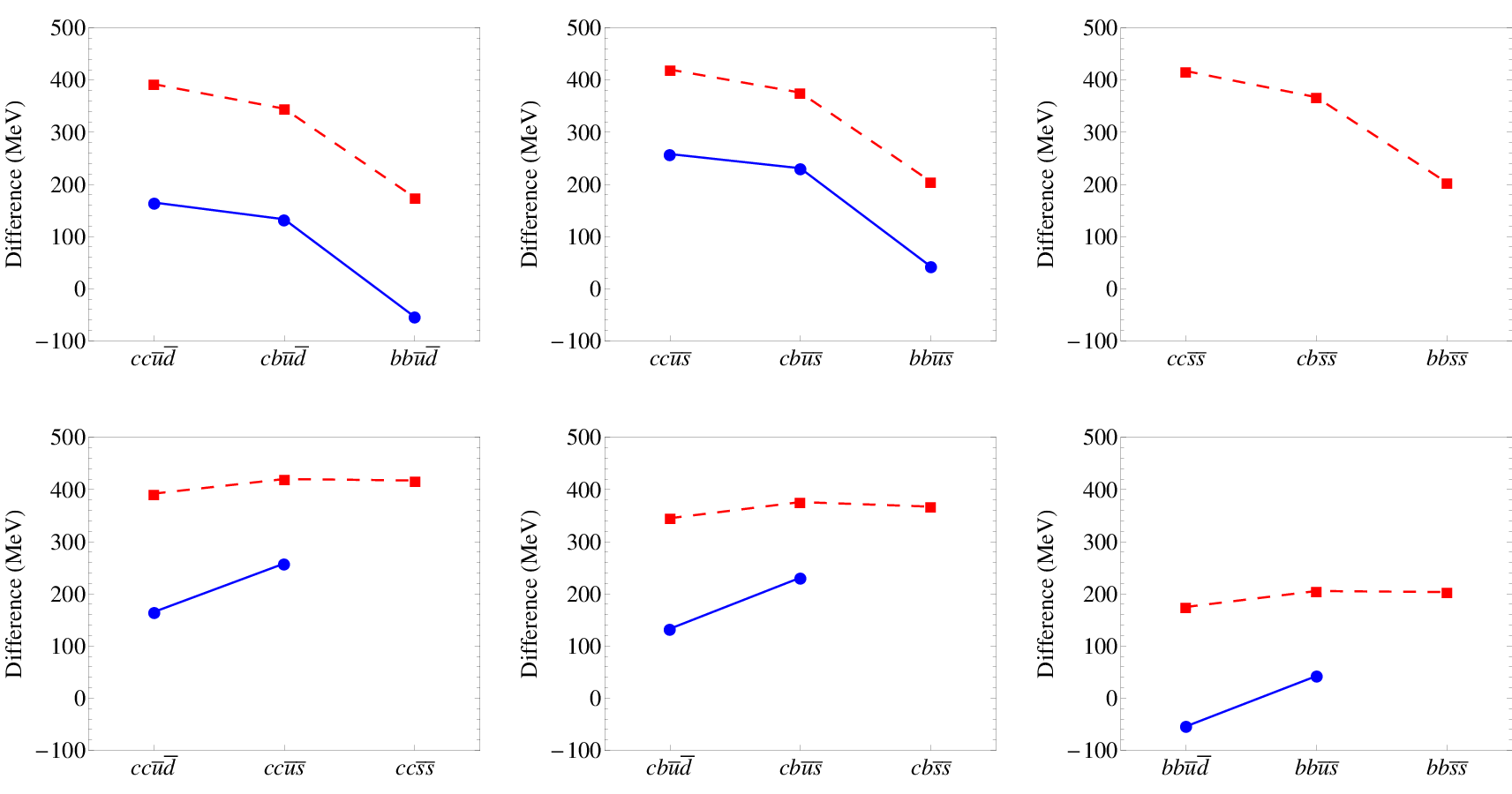
In Refs. Vijande:2009kj; Hernandez:2019eox, the authors also discussed the dependence of mass ratios between the heavy and light subsystems within nonrelativistic quark model, and showed the same behaviors with our relativized calculations. If one keeps reducing the mass ratios, the doubly heavy tetraquarks will become fully heavy tetraquarks. We can speculate that there is no stable state for the fully heavy tetraquarks since the mass ratios between the two subsystems are sufficiently small. This conjecture is supported by the experimental observations Aaij:2018zrb; Sirunyan:2020txn and nonrelativistic quark model works with proper potentials Richard:2017vry; Liu:2019zuc; Wang:2019rdo; Chen:2019vrj; Richard:2019cmi; Deng:2020iqw. Certainly, the classifications of fully heavy tetraquarks are different with doubly heavy tetraquarks, precise calculations within the relativized quark model are needed before coming to any conclusion.

IV Summary

In this work, we systematically investigate the mass spectra of doubly heavy tetraquarks $T_{QQ^{\prime}}$ in a relativized quark model. The four-body systems including the Coulomb potential, confining potential, spin-spin interactions, and relativistic corrections are solved within the variational method. With the present extension, the tetraquark, as well as the conventional hadrons can be described in a uniform frame. Our results suggest that the $IJ^{P}=01^{+}$ $bb\bar{u}\bar{d}$ state is 54 MeV below the relevant $\bar{B}\bar{B}$ and $\bar{B}\bar{B}^{*}$ thresholds, which indicates that both strong and electromagnetic decays are forbidden, and thus this state can be a stable one. The large hidden color component and small root mean square radius demonstrate that it is a compact tetraquark rather than a loosely bound molecule or point-like diquark-antidiquark structure. Compared with the results of nonrelativistic quark models, our calculations present a lower binding energy of this promising isoscalar $T_{bb}$ state, but the decay behaviors agree with each other. We believe our calculations and predictions of the doubly heavy tetraquarks may provide valuable information for future experimental searches.

ACKNOWLEDGEMENTS

We would like to thank Xian-Hui Zhong, Ming-Sheng Liu, and Wei Liang for helpful discussions. This project is supported by the National Natural Science Foundation of China under Grants No. 11705056, No. 11775050, No. 11947224, No. 11975245, and No. U1832173, by the fund provided to the Sino-German CRC 110 ”Symmetries and the Emergence of Structure in QCD” project by the NSFC under Grant No. 11621131001, and by the Key Research Program of Frontier Sciences, CAS, Grant No. Y7292610K1.

References

(1) M. Tanabashi et al. (Particle Data Group), Review of Particle Physics, Phys. Rev. D 98, 030001 (2018).
(2) H. X. Chen, W. Chen, X. Liu and S. L. Zhu, The hidden-charm pentaquark and tetraquark states, Phys. Rept. 639, 1 (2016).
(3) A. Hosaka, T. Iijima, K. Miyabayashi, Y. Sakai and S. Yasui, Exotic hadrons with heavy flavors: X, Y, Z, and related states, PTEP 2016, 062C01 (2016).
(4) J. M. Richard, Exotic hadrons: review and perspectives, Few Body Syst. 57, 1185 (2016).
(5) R. F. Lebed, R. E. Mitchell and E. S. Swanson, Heavy-Quark QCD Exotica, Prog. Part. Nucl. Phys. 93, 143-194 (2017).
(6) A. Ali, J. S. Lange and S. Stone, Exotics: Heavy Pentaquarks and Tetraquarks, Prog. Part. Nucl. Phys. 97, 123-198 (2017).
(7) A. Esposito, A. Pilloni and A. Polosa, Multiquark Resonances, Phys. Rept. 668, 1-97 (2017).
(8) F. K. Guo, C. Hanhart, U. G. Meißner, Q. Wang, Q. Zhao and B. S. Zou, Hadronic molecules, Rev. Mod. Phys. 90, 015004 (2018).
(9) S. L. Olsen, T. Skwarnicki and D. Zieminska, Nonstandard heavy mesons and baryons: Experimental evidence, Rev. Mod. Phys. 90, 015003 (2018).
(10) M. Karliner, J. L. Rosner and T. Skwarnicki, Multiquark States, Ann. Rev. Nucl. Part. Sci. 68, 17 (2018).
(11) Y. R. Liu, H. X. Chen, W. Chen, X. Liu and S. L. Zhu, Pentaquark and Tetraquark states, Prog. Part. Nucl. Phys. 107, 237 (2019).
(12) N. Brambilla, S. Eidelman, C. Hanhart, A. Nefediev, C. P. Shen, C. E. Thomas, A. Vairo and C. Z. Yuan, The $XYZ$ states: experimental and theoretical status and perspectives, arXiv:1907.07583.
(13) S. Choi et al. (Belle Collaboration), Observation of a resonance-like structure in the $\pi^{\pm}\psi^{\prime}$ mass distribution in exclusive $B\to K\pi^{\pm}\psi^{\prime}$ decays, Phys. Rev. Lett. 100, 142001 (2008).
(14) R. Aaij et al.(LHCb Collaboration), Observation of the resonant character of the $Z(4430)^{-}$ state, Phys. Rev. Lett. 112, 222002 (2014).
(15) A. Bondar et al. (Belle Collaboration), Observation of two charged bottomonium-like resonances in $\Upsilon(5S)$ decays, Phys. Rev. Lett. 108, 122001 (2012).
(16) M. Ablikim et al. (BESIII Collaboration), Observation of a Charged Charmoniumlike Structure in $e^{+}e^{-}\to\pi^{+}\pi^{-}J/\psi$ at $\sqrt{s}$ =4.26 GeV, Phys. Rev. Lett. 110, 252001 (2013).
(17) Z. Liu et al. (Belle Collaboration), Study of $e^{+}e^{-}\to\pi^{+}\pi^{-}J/\psi$ and Observation of a Charged Charmoniumlike State at Belle, Phys. Rev. Lett. 110, 252002 (2013).
(18) R. Aaij et al. (LHCb Collaboration), Observation of $J/\psi p$ Resonances Consistent with Pentaquark States in $\Lambda_{b}^{0}\to J/\psi K^{-}p$ Decays, Phys. Rev. Lett. 115, 072001 (2015).
(19) R. Aaij et al. (LHCb Collaboration), Observation of a narrow pentaquark state, $P_{c}(4312)^{+}$ , and of two-peak structure of the $P_{c}(4450)^{+}$ , Phys. Rev. Lett. 122, 222001 (2019).
(20) T. Nakano et al. (LEPS Collaboration), Evidence for a narrow $S=+1$ baryon resonance in photoproduction from the neutron, Phys. Rev. Lett. 91, 012002 (2003).
(21) V. Abazov et al. (D0 Collaboration), Evidence for a $B_{s}^{0}\pi^{\pm}$ state, Phys. Rev. Lett. 117, 022003 (2016).
(22) R. Aaij et al. (LHCb Collaboration), Search for Structure in the $B_{s}^{0}\pi^{\pm}$ Invariant Mass Spectrum, Phys. Rev. Lett. 117, 152003 (2016).
(23) R. Aaij et al. (LHCb Collaboration), Observation of the doubly charmed baryon $\Xi_{cc}^{++}$ , Phys. Rev. Lett. 119, 112001 (2017).
(24) M. Karliner and J. L. Rosner, Discovery of doubly-charmed $\Xi_{cc}$ baryon implies a stable ( $bb\bar{u}\bar{d}$ ) tetraquark, Phys. Rev. Lett. 119, 202001 (2017).
(25) E. J. Eichten and C. Quigg, Heavy-quark symmetry implies stable heavy tetraquark mesons $Q_{i}Q_{j}\bar{q}_{k}\bar{q}_{l}$ , Phys. Rev. Lett. 119, 202002 (2017).
(26) J. L. Ballot and J. M. Richard, Four Quark States In Additive Potentials, Phys. Lett. 123B, 449 (1983).
(27) H. J. Lipkin, A model-independent approach to multiquark bound states, Phys. Lett. B 172, 242 (1986).
(28) J. Vijande and A. Valcarce, Tetraquark Spectroscopy: A Symmetry Analysis, Symmetry 1, 155 (2009).
(29) S. Q. Luo, K. Chen, X. Liu, Y. R. Liu and S. L. Zhu, Exotic tetraquark states with the $qq\bar{Q}\bar{Q}$ configuration, Eur. Phys. J. C 77, 709 (2017).
(30) D. Ebert, R. N. Faustov, V. O. Galkin and W. Lucha, Masses of tetraquarks with two heavy quarks in the relativistic quark model, Phys. Rev. D 76, 114015 (2007).
(31) C. Semay and B. Silvestre-Brac, Diquonia and potential models, Z. Phys. C 61, 271 (1994).
(32) S. Zouzou, B. Silvestre-Brac, C. Gignoux and J. M. Richard, Four Quark Bound States, Z. Phys. C 30, 457 (1986).
(33) L. Heller and J. A. Tjon, On the Existence of Stable Dimesons, Phys. Rev. D 35, 969 (1987).
(34) J. Carlson, L. Heller and J. A. Tjon, Stability of Dimesons, Phys. Rev. D 37, 744 (1988).
(35) B. Silvestre-Brac and C. Semay, Systematics of $L=0$ $q^{2}\bar{q}^{2}$ systems, Z. Phys. C 57, 273 (1993).
(36) B. Silvestre-Brac and C. Semay, Spectrum and decay properties of diquonia, Z. Phys. C 59, 457 (1993).
(37) S. Pepin, F. Stancu, M. Genovese and J. M. Richard, Tetraquarks with color blind forces in chiral quark models, Phys. Lett. B 393, 119 (1997).
(38) D. M. Brink and F. Stancu, Tetraquarks with heavy flavors, Phys. Rev. D 57, 6778 (1998).
(39) J. Vijande, F. Fernandez, A. Valcarce and B. Silvestre-Brac, Tetraquarks in a chiral constituent quark model, Eur. Phys. J. A 19, 383 (2004).
(40) M. Zhang, H. X. Zhang and Z. Y. Zhang, $QQ\bar{q}\bar{q}$ four-quark bound states in chiral SU(3) quark model, Commun. Theor. Phys. 50, 437 (2008).
(41) J. Vijande, A. Valcarce and N. Barnea, Exotic meson-meson molecules and compact four-quark states, Phys. Rev. D 79, 074010 (2009).
(42) Y. C. Yang, C. R. Deng, J. L. Ping and T. Goldman, $S-$ wave $QQ\bar{q}\bar{q}$ state in the constituent quark model, Phys. Rev. D 80, 114023 (2009).
(43) F. S. Navarra, M. Nielsen and S. H. Lee, QCD sum rules study of $QQ-\bar{u}\bar{d}$ mesons, Phys. Lett. B 649, 166 (2007).
(44) J. M. Dias, S. Narison, F. S. Navarra, M. Nielsen, J.-M. Richard, Relation between $T_{cc,bb}$ and $X_{c,b}$ from QCD, Phys. Lett. B 703, 274 (2011).
(45) W. Chen, T. G. Steele and S. L. Zhu, Exotic open-flavor $bc\bar{q}\bar{q}$ , $bc\bar{s}\bar{s}$ and $qc\bar{q}\bar{b}$ , $sc\bar{s}\bar{b}$ tetraquark states, Phys. Rev. D 89, 054037 (2014).
(46) M. L. Du, W. Chen, X. L. Chen and S. L. Zhu, Exotic $QQ\bar{q}\bar{q}$ , $QQ\bar{q}\bar{s}$ and $QQ\bar{s}\bar{s}$ states, Phys. Rev. D 87, 014003 (2013).
(47) Y. Ikeda et al., Charmed tetraquarks $T_{cc}$ and $T_{cs}$ from dynamical lattice QCD simulations, Phys. Lett. B 729, 85 (2014).
(48) P. Bicudo, K. Cichy, A. Peters and M. Wagner, BB interactions with static bottom quarks from Lattice QCD, Phys. Rev. D 93, 034501 (2016).
(49) A. Francis, R. J. Hudspith, R. Lewis and K. Maltman, Lattice Prediction for Deeply Bound Doubly Heavy Tetraquarks, Phys. Rev. Lett. 118, 142001 (2017).
(50) P. Bicudo, M. Cardoso, A. Peters, M. Pflaumer and M. Wagner, $ud\bar{b}\bar{b}$ tetraquark resonances with lattice QCD potentials and the Born-Oppenheimer approximation, Phys. Rev. D 96, 054510 (2017).
(51) B. A. Gelman and S. Nussinov, Does a narrow tetraquark $cc\bar{u}\bar{d}$ state exist?, Phys. Lett. B 551, 296 (2003).
(52) D. Janc and M. Rosina, The $T_{cc}=DD^{*}$ molecular state, Few Body Syst. 35, 175 (2004).
(53) A. Del Fabbro, D. Janc, M. Rosina and D. Treleani, Production and detection of doubly charmed tetraquarks, Phys. Rev. D 71, 014008 (2005).
(54) Y. Q. Chen and S. Z. Wu, Production of four-quark states with double heavy quarks at LHC, Phys. Lett. B 705, 93 (2011).
(55) T. Hyodo, Y. R. Liu, M. Oka, K. Sudoh and S. Yasui, Production of doubly charmed tetraquarks with exotic color configurations in electron-positron collisions, Phys. Lett. B 721, 56-60 (2013).
(56) T. Mehen, Implications of Heavy Quark-Diquark Symmetry for Excited Doubly Heavy Baryons and Tetraquarks, Phys. Rev. D 96, 094028 (2017).
(57) Z. G. Wang and Z. H. Yan, Analysis of the scalar, axialvector, vector, tensor doubly charmed tetraquark states with QCD sum rules, Eur. Phys. J. C 78, 19 (2018).
(58) X. J. Yan, B. Zhong and R. L. Zhu, Doubly charmed tetraquarks in a diquark-antidiquark model, Int. J. Mod. Phys. A 33, 1850096 (2018).
(59) A. Ali, A. Y. Parkhomenko, Q. Qin and W. Wang, Prospects of discovering stable double-heavy tetraquarks at a Tera- $Z$ factory, Phys. Lett. B 782, 412 (2018).
(60) Y. Xing and R. Zhu, Weak Decays of Stable Doubly Heavy Tetraquark States, Phys. Rev. D 98, 053005 (2018).
(61) S. S. Agaev, K. Azizi, B. Barsbay and H. Sundu, The doubly charmed pseudoscalar tetraquarks $T_{cc;\bar{s}\bar{s}}^{++}$ and $T_{cc;\bar{d}\bar{s}}^{++}$ , Nucl. Phys. B 939, 130 (2019).
(62) A. Ali, Q. Qin and W. Wang, Discovery potential of stable and near-threshold doubly heavy tetraquarks at the LHC, Phys. Lett. B 785, 605 (2018).
(63) W. Park, S. Noh and S. H. Lee, Masses of the doubly heavy tetraquarks in a constituent quark model, Nucl. Phys. A 983, 1 (2019).
(64) S. S. Agaev, K. Azizi, B. Barsbay and H. Sundu, Weak decays of the axial-vector tetraquark $T_{bb;\bar{u}\bar{d}}^{-}$ , Phys. Rev. D 99, 033002 (2019).
(65) A. Francis, R. J. Hudspith, R. Lewis and K. Maltman, Evidence for charm-bottom tetraquarks and the mass dependence of heavy-light tetraquark states from lattice QCD, Phys. Rev. D 99, 054505 (2019).
(66) P. Junnarkar, N. Mathur and M. Padmanath, Study of doubly heavy tetraquarks in Lattice QCD, Phys. Rev. D 99, 034507 (2019).
(67) C. R. Deng, H. Chen and J. L. Ping, Systematical investigation on the stability of doubly heavy tetraquark states, Eur. Phys. J. A 56, 9 (2020).
(68) T. F. Carames, J. Vijande and A. Valcarce, Exotic $bc\bar{q}\bar{q}$ four-quark states, Phys. Rev. D 99, 014006 (2019).
(69) S. S. Agaev, K. Azizi and H. Sundu, Strong decays of double-charmed pseudoscalar and scalar $cc\overline{u}\overline{d}$ tetraquarks, Phys. Rev. D 99, 114016 (2019).
(70) H. Sundu, S. S. Agaev and K. Azizi, Semileptonic decays of the scalar tetraquark $Z_{bc;\overline{u}\overline{d}}^{0}$ , Eur. Phys. J. C 79, 753 (2019).
(71) L. Maiani, A. D. Polosa and V. Riquer, Hydrogen bond of QCD, Phys. Rev. D 100, 014002 (2019).
(72) R. L. Zhu, X. J. Liu, H. X. Huang and C. F. Qiao, Analyzing doubly heavy tetra- and penta-quark states by variational method, Phys. Lett. B 797, 134869 (2019).
(73) L. Maiani, A. D. Polosa and V. Riquer, Hydrogen bond of QCD in doubly heavy baryons and tetraquarks, Phys. Rev. D 100, 074002 (2019).
(74) C. E. Fontoura, G. Krein, A. Valcarce and J. Vijande, Production of exotic tetraquarks $QQ\bar{q}\bar{q}$ in heavy-ion collisions at the LHC, Phys. Rev. D 99, 094037 (2019).
(75) S. Agaev, K. Azizi and H. Sundu, Double-heavy axial-vector tetraquark $T_{bc;\bar{u}\bar{d}}^{0}$ , Nucl. Phys. B 951, 114890 (2020).
(76) L. Leskovec, S. Meinel, M. Pflaumer and M. Wagner, Lattice QCD investigation of a doubly-bottom $\bar{b}\bar{b}ud$ tetraquark with quantum numbers $I(J^{P})=0(1^{+})$ , Phys. Rev. D 100, 014503 (2019).
(77) Y. Liu, M. A. Nowak and I. Zahed, Heavy tetraquark $QQ\bar{q}\bar{q}$ as a hadronic Efimov state, arXiv:1909.02497.
(78) E. Hernandez, J. Vijande, A. Valcarce and J. M. Richard, Spectroscopy, lifetime and decay modes of the $T^{-}_{bb}$ tetraquark, Phys. Lett. B 800, 135073 (2020).
(79) G. Yang, J. L. Ping and J. Segovia, Doubly-heavy tetraquarks, Phys. Rev. D 101, 014001 (2020).
(80) L. Tang, B. D. Wan, K. Maltman and C. F. Qiao, Doubly Heavy Tetraquarks in QCD Sum Rules, arXiv:1911.10951.
(81) S. Agaev, K. Azizi, B. Barsbay and H. Sundu, Stable scalar tetraquark $T_{bb;\bar{u}\bar{d}}^{-}$ , arXiv:2001.01446.
(82) Q. N. Wang and W. Chen, Fully open-flavor tetraquark states $bc\bar{q}\bar{s}$ and $sc\bar{q}\bar{b}$ with $J^{P}=0^{+},1^{+}$ , Eur. Phys. J. C 80, 389 (2020).
(83) Y. Tan, W. Lu and J. L. Ping, $QQ\bar{q}\bar{q}$ in a chiral constituent quark model, arXiv:2004.02106.
(84) S. Godfrey and N. Isgur, Mesons in a Relativized Quark Model with Chromodynamics, Phys. Rev. D 32, 189 (1985).
(85) S. Capstick and N. Isgur, Baryons in a Relativized Quark Model with Chromodynamics, Phys. Rev. D 34, 2809 (1986).
(86) Q. F. Lü and Y. B. Dong, $X(4140)$ , $X(4274)$ , $X(4500)$ , and $X(4700)$ in the relativized quark model, Phys. Rev. D 94, 074007 (2016).
(87) Q. F. Lü and Y. B. Dong, Masses of open charm and bottom tetraquark states in a relativized quark model, Phys. Rev. D 94, 094041 (2016).
(88) Q. F. Lü, K. L. Wang and Y. B. Dong, The $ss\bar{s}\bar{s}$ tetraquark states and the newly observed structure $X(2239)$ by BESIII Collaboration, Chin. Phys. C 44, 024101 (2020).
(89) M. N. Anwar, J. Ferretti, F. K. Guo, E. Santopinto and B. S. Zou, Spectroscopy and decays of the fully-heavy tetraquarks, Eur. Phys. J. C 78, 647 (2018).
(90) M. N. Anwar, J. Ferretti and E. Santopinto, Spectroscopy of the hidden-charm $[qc][\bar{q}\bar{c}]$ and $[sc][\bar{s}\bar{c}]$ tetraquarks in the relativized diquark model, Phys. Rev. D 98, 094015 (2018).
(91) M. A. Bedolla, J. Ferretti, C. D. Roberts and E. Santopinto, Spectrum of fully-heavy tetraquarks from a diquark+antidiquark perspective, arXiv:1911.00960.
(92) J. Ferretti and E. Santopinto, Hidden-charm and bottom tetra- and pentaquarks with strangeness in the hadro-quarkonium and compact tetraquark models, JHEP 04, 119 (2020).
(93) E. Hiyama, Y. Kino and M. Kamimura, Gaussian expansion method for few-body systems, Prog. Part. Nucl. Phys. 51, 223 (2003).
(94) R. Aaij et al. (LHCb Collaboration), Physics case for an LHCb Upgrade II - Opportunities in flavour physics, and beyond, in the HL-LHC era, arXiv:1808.08865.
(95) A. Cerri et al., Opportunities in Flavour Physics at the HL-LHC and HE-LHC, CERN Yellow Rep. Monogr. 7, 867-1158 (2019).
(96) R. Aaij et al. (LHCb Collaboration), Search for beautiful tetraquarks in the $\Upsilon(1S)\mu^{+}\mu^{-}$ invariant-mass spectrum, JHEP 10, 086 (2018).
(97) A. M. Sirunyan et al. (CMS Collaboration), Measurement of the $\Upsilon$ (1S) pair production cross section and search for resonances decaying to $\Upsilon(1S)\mu^{+}\mu^{-}$ in proton-proton collisions at $\sqrt{s}=$ 13 TeV, arXiv:2002.06393.
(98) J. M. Richard, A. Valcarce and J. Vijande, String dynamics and metastability of all-heavy tetraquarks, Phys. Rev. D 95, 054019 (2017).
(99) M. S. Liu, Q. F. Lü, X. H. Zhong and Q. Zhao, All-heavy tetraquarks, Phys. Rev. D 100, 016006 (2019).
(100) G. J. Wang, L. Meng and S. L. Zhu, Spectrum of the fully-heavy tetraquark state $QQ\bar{Q}^{\prime}\bar{Q}^{\prime}$ , Phys. Rev. D 100, 096013 (2019).
(101) X. Y. Chen, Fully-heavy tetraquarks: $bb\bar{c}\bar{c}$ and $bc\bar{b}\bar{c}$ , Phys. Rev. D 100, 094009 (2019).
(102) J. M. Richard, A. Valcarce and J. Vijande, Hall¨CPost inequalities: Review and application to molecules and tetraquarks, Annals Phys. 412, 168009 (2020).
(103) C. R. Deng, H. Chen and J. L. Ping, Towards the understanding of fully-heavy tetraquark states from various models, arXiv:2003.05154.

Masses of doubly heavy tetraquarks TQ​Q′T_{QQ^{\prime}} in a relativized quark model

Abstract

I Introduction

II Model

II.1 Hamiltonian

II.2 Matrix elements of color, flavor, and spin parts

II.3 Matrix elements of spatial part

II.4 Generalized eigenvalue problem

III RESULTS AND DISCUSSIONS

III.1 Numerical stability

III.2 Non-strange systems

III.3 Strange systems

III.4 Mass ratios

IV Summary

References

Masses of doubly heavy tetraquarks $T_{QQ^{\prime}}$ in a relativized quark model