跳到论文正文
W Papers独立论文阅读器 arXiv:2006.08085 论文正文 计算阅读时间 · 0%
引用这篇论文根据当前论文元数据生成,正式投稿前建议核对。


License: CC BY-NC-ND 4.0
arXiv:2006.08085v4 [cs.LG] 28 Jan 2022

Optimal Complexity in Decentralized Training

Yucheng Lu Thanks: Corresponds to: yl2967@cornell.edu Affiliation: Department of Computer Science, Cornell University    Christopher De Sa Thanks: Corresponds to: cdesa@cs.cornell.edu Affiliation: Department of Computer Science, Cornell University
Abstract

Decentralization is a promising method of scaling up parallel machine learning systems. In this paper, we provide a tight lower bound on the iteration complexity for such methods in a stochastic non-convex setting. Our lower bound reveals a theoretical gap in known convergence rates of many existing decentralized training algorithms, such as D-PSGD. We prove by construction this lower bound is tight and achievable. Motivated by our insights, we further propose DeTAG, a practical gossip-style decentralized algorithm that achieves the lower bound with only a logarithm gap. Empirically, we compare DeTAG with other decentralized algorithms on image classification tasks, and we show DeTAG enjoys faster convergence compared to baselines, especially on unshuffled data and in sparse networks.

1 Introduction

Parallelism is a ubiquitous method to accelerate model training [1, 2, 3, 4]. A parallel learning system usually consists of three layers (Table 1): an application to solve, a communication protocol deciding how parallel workers coordinate, and a network topology determining how workers are connected. Traditional design for these layers usually follows a centralized setup: in the application layer, training data is required to be shuffled and shared among parallel workers; while in the protocol and network layers, workers either communicate via a fault-tolerant single central node (e.g. Parameter Server) [5, 6, 7] or a fully-connected topology (e.g. AllReduce) [8, 9]. This centralized design limits the scalability of learning systems in two aspects. First, in many scenarios, such as Federated Learning [10, 11] and Internet of Things (IOT) [12], a shuffled dataset or a complete (bipartite) communication graph is not possible or affordable to obtain. Second, a centralized communication protocol can significantly slow down the training, especially with a low-bandwidth or high-latency network [13, 14, 15].

Table 1: Design choice of centralization and decentralization in different layers of a parallel machine learning system. The protocol specifies how workers communicate. The topology refers to the overlay network that logically connects all the workers.
Layer Centralized Decentralized
Application Shuffled Data Unshuffled Data
(Federated Learning)
Protocol AllReduce/AllGather Gossip
Parameter Server
Network Complete- Arbitrary Graph
Topology (Bipartite) Graph

The rise of decentralization. To mitigate these limitations, decentralization comes to the rescue. Decentralizing the application and network allows workers to learn with unshuffled local datasets [16] and arbitrary topologies [17, 18]. Furthermore, the decentralized protocol, i.e. Gossip, helps to balance load, and has been shown to outperform centralized protocols in many cases [19, 20, 21, 22].

Understanding decentralization with layers. Many decentralized training designs have been proposed, which can lead to confusion as the term “decentralization” is used inconsistently in the literature. Some works use “decentralized” to refer to approaches that can tolerate non-iid or unshuffled datasets [16], while others use it to mean gossip communication [19], and still others use it to mean a sparse topology graph [23]. To eliminate this ambiguity, we formulate Table 1, which summarizes the different “ways” a system can be decentralized. Note that the choices to decentralize different layers are independent, e.g., the centralized protocol AllReduce can still be implemented on a decentralized topology like the Ring graph [23].

Refer to caption
Figure 1: Figure illustrating how decentralization in different layers lead to different learning systems. From left to right: : A fully centralized system where workers sample from shared and shuffled data; ②: Based on ①, workers maintain their own data sources, making it decentralized in the application layer; ③: Based on ②, workers are decentralized in the topology layer; ④: A fully decentralized system in all three layers where the workers communicate via Gossip. Our framework and theory are applicable to all kinds of decentralized learning systems.

The theoretical limits of decentralization. Despite the empirical success, the best convergence rates achievable by decentralized training—and how they interact with different notions of decentralization—remains an open question. Previous works often show complexity of a given decentralized algorithm with respect to the number of iterations TT or the number of workers nn, ignoring other factors including network topologies, function parameters or data distribution. Although a series of decentralized algorithms have been proposed showing theoretical improvements—such as using variance reduction [24], acceleration [17], or matching [25]—we do not know how close they are to an “optimal” rate or whether further improvement is possible.

In light of this, a natural question is: What is the optimal complexity in decentralized training? Has it been achieved by any algorithm yet? Previous works have made initial attempts on this question, by analyzing this theoretical limit in a non-stochastic or (strongly) convex setting [17, 26, 27, 28, 29, 30]. These results provide great heuristics but still leave the central question open, since stochastic methods are usually used in practice and many real-world problems of interest are non-convex (e.g. deep learning). In this paper we give the first full answer to this question: our contributions are as follows.

  • •

    In Section 4, we prove the first (to our knowledge) tight lower bound for decentralized training in a stochastic non-convex setting. Our results reveal an asymptotic gap between our lower bound and known convergence rates of existing algorithms.

  • •

    In Section 5, we prove our lower bound is tight by exhibiting an algorithm called DeFacto that achieves it—albeit while only being decentralized in the sense of the application and network layers.

  • •

    In Section 6, we propose DeTAG, a practical algorithm that achieves the lower bound with only a logarithm gap and that is decentralized in all three layers.

  • •

    In Section 7, we experimentally evaluate DeTAG on the CIFAR benchmark and show it converges faster compared to decentralized learning baselines.

2 Related Work

Decentralized Training. In the application layer, decentralized training usually denotes federated learning [31]. Research on decentralization in this sense investigates convergence where each worker samples only from a local dataset which is not independent and identically distributed to other workers’ datasets [32, 33, 34, 35]. Another line of research on decentralization focuses on the protocol layer—with average gossip [36, 37], workers communicate by averaging their parameters with neighbors on a graph. D-PSGD [19] is one of the most basic algorithms that scales SGD with this protocol, achieving a linear parallel speed up. Additional works extend D-PSGD to asynchronous and variance-reduced cases [13, 24, 38, 39, 40, 41]. After those, Zhang and You 2019b, Xin et al. 2019, Xin et al. 2021b propose adding gradient trackers to D-PSGD. Other works discuss the application of decentralization on specific tasks such as linear models or deep learning [45, 46]. Zhang and You 2019c treats the case where only directed communication can be performed. Wang et al. 2019 proposes using matching algorithms to optimize the gossip protocol. Multiple works discuss using compression to decrease communication costs in decentralized training [48, 10, 22, 49, 50], and other papers connect decentralized training to other parallel methods and present a unified theory [4, 27, 51]. In some even earlier works like [52, 53], full local gradients on a convex setting is investigated.

Lower Bounds in Stochastic Optimization. Lower bounds are a well studied topic in non-stochastic optimization, especially in convex optimization [54, 55, 56, 57, 58]. In the stochastic setting, Allen-Zhu 2018 and Foster et al. 2019 discuss the complexity lower bound to find stationary points on convex problems. Other works study the lower bound in a convex, data-parallel setting [61, 62, 63], and Colin et al. 2019 extends the result to a model-parallel setting. In the domain of non-convex optimization, Carmon et al. 2017, Carmon et al. 2019 propose a zero-chain model that obtains tight bound for a first order method to obtain stationary points. Zhou and Gu 2019 extends this lower bound to a finite sum setting, and Arjevani et al. 2019 proposes a probabilistic zero-chain model that obtains tight lower bounds for first-order methods on stochastic and non-convex problems.

Table 2: Complexity comparison among different algorithms in the stochastic non-convex setting on arbitrary graphs. The blue text are the results from this paper. Definitions to all the parameters can be found in Section 3. Other algorithms like EXTRA [69] or MSDA [70] are not comparable since they are designed for (strongly) convex problems. Additionally, Liu and Zhang 2021 provides alternative complexity bound for algorithms like D-PSGD which improves upon the spectral gap. However, the new bound would compromise the dependency on ϵ\epsilon, which does not conflict with our comparison here.
Source Protocol Sample Complexity Comm. Complexity Gap to Lower Bound
Lower Bound Theorem 1 Central Ω⁡(Δ​L​σ2n​B​ϵ4)\Omega\left(\frac{\Delta L\sigma^{2}}{nB\epsilon^{4}}\right) Ω⁡(Δ​L​Dϵ2)\Omega\left(\frac{\Delta LD}{\epsilon^{2}}\right) /
Corollary 1 Decentral Ω⁡(Δ​L​σ2n​B​ϵ4)\Omega\left(\frac{\Delta L\sigma^{2}}{nB\epsilon^{4}}\right) Ω⁡(Δ​Lϵ2​1−λ)\Omega\left(\frac{\Delta L}{\epsilon^{2}\sqrt{1-\lambda}}\right) /
Upper Bound DeFacto (Theorem 2) Central O⁡(Δ​L​σ2n​B​ϵ4)O\left(\frac{\Delta L\sigma^{2}}{nB\epsilon^{4}}\right) O⁡(Δ​L​Dϵ2)O\left(\frac{\Delta LD}{\epsilon^{2}}\right) O⁡(1)O(1)
DeTAG (Theorem 3) Decentral O⁡(Δ​L​σ2n​B​ϵ4)O\left(\frac{\Delta L\sigma^{2}}{nB\epsilon^{4}}\right) O⁡(Δ​L​log⁡(ς0​nϵ​Δ​L)ϵ2​1−λ){\color[rgb]{0,0,1}O\left(\frac{\Delta L\log\left(\frac{\varsigma_{0}n}{\epsilon\sqrt{\Delta L}}\right)}{\epsilon^{2}\sqrt{1-\lambda}}\right)} O⁡(log⁡(ς0​nϵ​Δ​L))O\left(\log\left(\frac{\varsigma_{0}n}{\epsilon\sqrt{\Delta L}}\right)\right)
D-PSGD [19] Decentral O⁡(Δ​L​σ2n​B​ϵ4)O\left(\frac{\Delta L\sigma^{2}}{nB\epsilon^{4}}\right) O⁡(Δ​L​n​ςϵ2​(1−λ)2)O\left(\frac{\Delta Ln\varsigma}{\epsilon^{2}(1-\lambda)^{2}}\right) O⁡(n​ς(1−λ)32)O\left(\frac{n\varsigma}{(1-\lambda)^{\frac{3}{2}}}\right)
SGP [72] Decentral O⁡(Δ​L​σ2n​B​ϵ4)O\left(\frac{\Delta L\sigma^{2}}{nB\epsilon^{4}}\right) O⁡(Δ​L​n​ςϵ2​(1−λ)2)O\left(\frac{\Delta Ln\varsigma}{\epsilon^{2}(1-\lambda)^{2}}\right) O⁡(n​ς(1−λ)32)O\left(\frac{n\varsigma}{(1-\lambda)^{\frac{3}{2}}}\right)
D2 [24] Decentral O⁡(Δ​L​σ2n​B​ϵ4)O\left(\frac{\Delta L\sigma^{2}}{nB\epsilon^{4}}\right) O⁡(λ2​Δ​L​n​ς0ϵ2​(1−λ)3)O\left(\frac{\lambda^{2}\Delta Ln\varsigma_{0}}{\epsilon^{2}(1-\lambda)^{3}}\right) O⁡(λ2​n​ς0(1−λ)52)O\left(\frac{\lambda^{2}n\varsigma_{0}}{(1-\lambda)^{\frac{5}{2}}}\right)
DSGT [42] Decentral O⁡(Δ​L​σ2n​B​ϵ4)O\left(\frac{\Delta L\sigma^{2}}{nB\epsilon^{4}}\right) O⁡(λ2​Δ​L​n​ς0ϵ2​(1−λ)3)O\left(\frac{\lambda^{2}\Delta Ln\varsigma_{0}}{\epsilon^{2}(1-\lambda)^{3}}\right) O⁡(λ2​n​ς0(1−λ)52)O\left(\frac{\lambda^{2}n\varsigma_{0}}{(1-\lambda)^{\frac{5}{2}}}\right)
GT-DSGD [44] Decentral O⁡(Δ​L​σ2n​B​ϵ4)O\left(\frac{\Delta L\sigma^{2}}{nB\epsilon^{4}}\right) O⁡(λ2​Δ​L​n​ς0ϵ2​(1−λ)3)O\left(\frac{\lambda^{2}\Delta Ln\varsigma_{0}}{\epsilon^{2}(1-\lambda)^{3}}\right) O⁡(λ2​n​ς0(1−λ)52)O\left(\frac{\lambda^{2}n\varsigma_{0}}{(1-\lambda)^{\frac{5}{2}}}\right)

3 Setting

In this section, we introduce the notation and assumptions we will use. Throughout the paper, we consider the standard data-parallel training setup with nn parallel workers. Each worker ii stores a copy of the model 𝒙∈ℝd\boldsymbol{x}\in\mathbb{R}^{d} and a local dataset 𝒟i\mathcal{D}_{i}. The model copy and local dataset define a local loss function (or empirical risk) fif_{i}. The ultimate goal of the parallel workers is to output a target model 𝒙^\boldsymbol{\hat{x}} that minimizes the average over all the local loss functions, that is,

𝒙^=argmin𝒙∈ℝd[f(𝒙)=1n∑i=1n𝔼ξi∼𝒟i​fi​(𝒙,ξi)⏟fi​(𝒙)].\boldsymbol{\hat{x}}=\arg\min_{\boldsymbol{x}\in\mathbb{R}^{d}}\left[f(\boldsymbol{x})=\frac{1}{n}\sum_{i=1}^{n}\underbrace{\mathbb{E}_{\xi_{i}\sim\mathcal{D}_{i}}f_{i}(\boldsymbol{x};\xi_{i})}_{f_{i}(\boldsymbol{x})}\right]. (1)

Here, ξi\xi_{i} is a data sample from 𝒟i\mathcal{D}_{i} and is used to compute a stochastic gradient via some oracle, e.g. back-propagation on a mini-batch of samples. The loss functions can (potentially) be non-convex so finding a global minimum is NP-Hard; instead, we expect the workers to output a point 𝒙^\boldsymbol{\hat{x}} at which f⁡(𝒙^)f(\boldsymbol{\hat{x}}) has a small gradient magnitude in expectation: 𝔼​‖∇f​(𝒙^)‖≤ϵ\mathbb{E}\|\nabla f(\boldsymbol{\hat{x}})\|\leq\epsilon, for some small ϵ\epsilon.11 1 There are many valid stopping criteria. We adopt ϵ\epsilon-stationary point as the success signal. 𝔼​‖∇f​(𝒙^)‖2≤ϵ2\mathbb{E}\|\nabla f(\boldsymbol{\hat{x}})\|^{2}\leq\epsilon^{2} is another commonly used criterion; we adopt the non-squared one following [66]. Other criterions regarding stationary points can be converted to hold in our theory. The assumptions our theoretical analysis requires can be categorized by the layers from Table 1: in each layer, “being decentralized” corresponds to certain assumptions (or lack of assumptions). We now describe these assumptions for each layer separately.

3.1 Application Layer

Application-layer assumptions comprise constraints on the losses fif_{i} from (1) and the gradient oracle via which they are accessed by the learning algorithm, as these are constraints on the learning task itself.

Function class (Δ\Delta and LL). As is usual in this space, we assume the local loss functions fi:ℝd→ℝf_{i}:\mathbb{R}^{d}\rightarrow\mathbb{R} are LL-smooth,

‖∇fi​(𝒙)−∇fi​(𝒚)‖≤L​‖𝒙−𝒚‖,∀𝒙,𝒚∈ℝd,\|\nabla f_{i}(\boldsymbol{x})-\nabla f_{i}(\boldsymbol{y})\|\leq L\|\boldsymbol{x}-\boldsymbol{y}\|,\;\forall\boldsymbol{x},\boldsymbol{y}\in\mathbb{R}^{d}, (2)

for some constant L>0L>0, and that the total loss ff is range-bounded by Δ\Delta in the sense that f⁡(𝟎)−inf𝒙f⁡(𝒙)≤Δf(\boldsymbol{0})-\inf_{\boldsymbol{x}}f(\boldsymbol{x})\leq\Delta. We let the function class ℱΔ,L\mathcal{F}_{\Delta,L} denote the set of all functions that satisfy these conditions (for any dimension d∈ℕ+d\in\mathbb{N}^{+}).

Oracle class (σ2\sigma^{2}). We assume each worker interacts with its local function fif_{i} only via a stochastic gradient oracle g~i\tilde{g}_{i}, and that when we query this oracle with model 𝒙\boldsymbol{x}, it returns an independent unbiased estimator to ∇fi​(𝒙)\nabla f_{i}(\boldsymbol{x}) based on some random variable zz with distribution ZZ (e.g. the index of a mini-batch randomly chosen for backprop). Formally,

𝔼z∼Z​[g~i​(𝒙,z)]=∇fi​(𝒙),∀𝒙∈ℝd.\mathbb{E}_{z\sim Z}[\tilde{g}_{i}(\boldsymbol{x},z)]=\nabla f_{i}(\boldsymbol{x}),\;\forall\boldsymbol{x}\in\mathbb{R}^{d}. (3)

As per the usual setup, we additionally assume the local estimator has bounded variance: for some constant σ>0\sigma>0,

𝔼z∼Z​‖g~i​(𝒙,z)−∇fi​(𝒙)‖2≤σ2,∀𝒙∈ℝd.\mathbb{E}_{z\sim Z}\|\tilde{g}_{i}(\boldsymbol{x},z)-\nabla f_{i}(\boldsymbol{x})\|^{2}\leq\sigma^{2},\;\forall\boldsymbol{x}\in\mathbb{R}^{d}. (4)

We let OO denote a set of these oracles {g~i}i∈[n]\{\tilde{g}_{i}\}_{i\in[n]}, and let the oracle class 𝒪σ2\mathcal{O}_{\sigma^{2}} denote the class of all such oracle sets that satisfy these two assumptions.

Data shuffling (ς2\varsigma^{2} and ς02\varsigma_{0}^{2}). At this point, an analysis with a centralized application layer would make the additional assumption that all the fif_{i} are equal and the g~i\tilde{g}_{i} are identically distributed: this roughly corresponds to the assumption that the data all comes independently from a single centralized source. We do not make this assumption, and lacking such an assumption is what makes an analysis decentralized in the application layer. Still, some assumption that bounds the fif_{i} relative to each other somehow is needed: we now discuss two such assumptions used in the literature, from which we use the weaker (and more decentralized) one.

One commonly made assumption [19, 48, 10, 22, 50] in decentralized training is

1n​∑i=1n‖∇fi​(𝒙)−∇f​(𝒙)‖2≤ς2,∀𝒙∈ℝd,\frac{1}{n}\sum_{i=1}^{n}\|\nabla f_{i}(\boldsymbol{x})-\nabla f(\boldsymbol{x})\|^{2}\leq\varsigma^{2},\;\forall\boldsymbol{x}\in\mathbb{R}^{d}, (5)

for some constant ς\varsigma, which is said to bound the “outer variance” among workers. This is often unreasonable, as it suggests the local datasets on workers must have close distribution: in practice, ensuring this often requires some sort of shuffling or common centralized data source. We do not assume (5) but instead adopt the much weaker assumption

1n​∑i=1n‖∇fi​(𝟎)−∇f​(𝟎)‖2≤ς02,\frac{1}{n}\sum_{i=1}^{n}\|\nabla f_{i}(\boldsymbol{0})-\nabla f(\boldsymbol{0})\|^{2}\leq\varsigma_{0}^{2}, (6)

for constant ς0>0\varsigma_{0}>0.22 2 As we only use ς0\varsigma_{0} for upper bounds, not lower bounds, we do not define a “class” that depends on this parameter. This assumption only requires a bound at point 𝟎\boldsymbol{0}, which is, to the best of our knowledge, the weakest assumption of this type used in the literature [24, 42]. Requiring such a weak assumption allows workers to (potentially) sample from different distributions or vary largely in their loss functions (e.g. in a federated learning environment).

3.2 Protocol Layer

Protocol-layer assumptions comprise constraints on the parallel learning algorithm itself, and especially on the way that the several workers communicate to approach consensus.

Algorithm class (BB). We consider algorithms AA that divide training into multiple iterations, and between two adjacent iterations, there must be a synchronization process among workers (e.g. a barrier) such that they start each iteration simultaneously.33 3 We consider synchronous algorithms only here for simplicity of presentation; further discussion of extension to asynchronous algorithms is included in the supplementary material. Each worker running AA has a local copy of the model, and we let 𝒙t,i∈ℝd\boldsymbol{x}_{t,i}\in\mathbb{R}^{d} denote this model on worker ii at iteration tt. We assume without loss of generality that AA initializes each local model at zero: 𝒙0,i=𝟎\boldsymbol{x}_{0,i}=\boldsymbol{0} for all ii. At each iteration, each worker makes at most BB queries to its gradient oracle g~i\tilde{g}_{i}, for some constant B∈ℕ+B\in\mathbb{N}^{+}, and then uses the resulting gradients to update its model. We do not make any explicit rules for output and allow the output of the algorithm 𝒙^t\boldsymbol{\hat{x}}_{t} at the end of iteration tt (the model that AA would output if it were stopped at iteration tt) to be any linear combination of all the local models, i.e.

𝒙^t∈span​({𝒙t,j}j∈[n])={∑j=1ncj​𝒙t,j∣cj∈ℝ}.\textstyle\boldsymbol{\hat{x}}_{t}\in\text{span}(\{\boldsymbol{x}_{t,j}\}_{j\in[n]})=\{\sum_{j=1}^{n}c_{j}\boldsymbol{x}_{t,j}\mid c_{j}\in\mathbb{R}\}. (7)

Beyond these basic properties, we further require AA to satisfy the following “zero-respecting” property from Carmon et al. 2017. Specifically, if 𝒛\boldsymbol{z} is any vector worker ii queries its gradient oracle with at iteration tt, then for any k∈[d]k\in[d], if 𝒆k⊤​𝒛≠0\boldsymbol{e}_{k}^{\top}\boldsymbol{z}\neq 0, then there exists a s≤ts\leq t and a j∈[n]j\in[n] such that either j=ij=i or jj is a neighbor of ii in the network connectivity graph GG (i.e. (i,j)∈{(i,i)}∪G(i,j)\in\{(i,i)\}\cup G) and (𝒆k⊤​𝒙s,j)≠0(\boldsymbol{e}_{k}^{\top}\boldsymbol{x}_{s,j})\neq 0. More informally, the worker will not query its gradient oracle with a nonzero value for some weight unless that weight was already nonzero in the model state of the worker or one of its neighbors at some point in the past. Similarly, for any k∈[d]k\in[d], if (𝒆k⊤​𝒙t+1,i)≠0(\boldsymbol{e}_{k}^{\top}\boldsymbol{x}_{t+1,i})\neq 0, then either there exists an s≤ts\leq t and jj such that (i,j)∈{(i,i)}∪G(i,j)\in\{(i,i)\}\cup G and (𝒆k⊤​𝒙s,j)≠0(\boldsymbol{e}_{k}^{\top}\boldsymbol{x}_{s,j})\neq 0, or one of the gradient oracle’s outputs 𝒗\boldsymbol{v} on worker ii at iteration tt has 𝒆k⊤​𝒗≠0\boldsymbol{e}_{k}^{\top}\boldsymbol{v}\neq 0. Informally, a worker’s model will not have a nonzero weight unless either (1) that weight was nonzero on that worker or one of its neighbors at a previous iteration, or (2) the corresponding entry in one of the gradients the worker sampled at that iteration was nonzero.

Intuitively, we are requiring that algorithm AA will not modify those coordinates that remain zero in all previous oracle outputs and neighboring models.44 4 On the other hand, it is possible to even drop the zero-respecting requirement and extend AA to all the deterministic (not in the sense of sampling but the actual executions) algorithms. At a cost, we would need the function class to follow an “orthogonal invariant” property, and the model dimension needs to be large enough. We leave this discussion to the appendix. This lets AA use a wide space of accessible information in communication and allows our class to cover first-order methods including SGD [73], Momentum SGD [74], Adam [75], RMSProp [76], Adagrad [77], and AdaDelta [78]. We let algorithm class 𝒜B\mathcal{A}_{B} denote the set of all algorithms AA that satisfy these assumptions.

So far our assumptions in this layer cover both centralized and decentralized protocols. Decentralized protocols, however, must satisfy the additional assumption that they communicate via gossip (see Section 2) [36, 37]. A single step of gossip protocol can be expressed as

𝒛t,i←∑j∈𝒩i𝒚t,j​𝑾j​i,∀i∈[n]\textstyle\boldsymbol{z}_{t,i}\leftarrow\sum_{j\in\mathcal{N}_{i}}\boldsymbol{y}_{t,j}\boldsymbol{W}_{ji},\;\forall i\in[n] (8)

for some constant doubly stochastic matrix 𝑾∈ℝn×n\boldsymbol{W}\in\mathbb{R}^{n\times n} called the communication matrix and 𝒚\boldsymbol{y} and 𝒛\boldsymbol{z} are the input and output of the gossip communication step, respectively. The essence of a single Gossip step is to take weighted average over the neighborhood specified by a fixed matrix. To simplify later discussion, we further define the gossip matrix class 𝒲n\mathcal{W}_{n} as the set of all matrices 𝑾∈ℝn×n\boldsymbol{W}\in\mathbb{R}^{n\times n}, where 𝑾\boldsymbol{W} is doubly stochastic and 𝑾i​j≠0\boldsymbol{W}_{ij}\neq 0 only if (i,j)∈G(i,j)\in G. We call every 𝑾∈𝒲n\boldsymbol{W}\in\mathcal{W}_{n} a gossip matrix and we use λ=max⁡{|λ2|,|λn|}∈[0,1)\lambda=\max\{|\lambda_{2}|,|\lambda_{n}|\}\in[0,1) to denote its general second-largest eigenvalue, where λi\lambda_{i} denotes the ii-th largest eigenvalue of 𝑾\boldsymbol{W}. We let gossip algorithm class 𝒜B,𝑾\mathcal{A}_{B,\boldsymbol{W}} denote the set of all algorithms A∈𝒜BA\in\mathcal{A}_{B} that only communicate via gossip using a single matrix 𝑾∈𝒲n\boldsymbol{W}\in\mathcal{W}_{n}. It trivially holds that 𝒜B,𝑾⊂𝒜B\mathcal{A}_{B,\boldsymbol{W}}\subset\mathcal{A}_{B}.

3.3 Topology Layer

Topology-layer assumptions comprise constraints on how workers are connected topologically. We let the graph class 𝒢n,D\mathcal{G}_{n,D} denote the class of graphs GG connecting nn workers (vertices) with diameter DD, where diameter of a graph measures the maximum distance between two arbitrary vertices (so 1≤D≤n−11\leq D\leq n-1). A centralized analysis here typically will also require that GG be either complete or complete-bipartite (with parameter servers and workers as the two parts): lacking this requirement and allowing arbitrary graphs is what makes an analysis decentralized in the topology layer.

3.4 Complexity Measures

Now that we have defined the classes we are interested in, we can use them to define the complexity measures we will bound in our theoretical results. Given a loss function f∈ℱΔ,Lf\in\mathcal{F}_{\Delta,L}, a set of underlying oracles O∈𝒪σ2O\in\mathcal{O}_{\sigma^{2}}, a graph G∈𝒢n,DG\in\mathcal{G}_{n,D}, and an algorithm A∈𝒜BA\in\mathcal{A}_{B}, let 𝒙^tA,f,O,G\boldsymbol{\hat{x}}_{t}^{A,f,O,G} denote the output of algorithm AA at the end of iteration tt under this setting. Then the iteration complexity of AA solving ff under OO and GG is defined as

Tϵ​(A,f,O,G)=min⁡{t∈ℕ|𝔼⁡‖∇f​(𝒙^tA,f,O,G)‖≤ϵ},T_{\epsilon}(A,f,O,G)=\min\left\{t\in\mathbb{N}\,\middle|\,\mathbb{E}\left\|\nabla f(\boldsymbol{\hat{x}}_{t}^{A,f,O,G})\right\|\leq\epsilon\right\},

that is, the least number of iterations required by AA to find a ϵ\epsilon-stationary-in-expectation point of ff.

4 Lower Bound

Given the setup in Section 3, we can now present and discuss our lower bound on the iteration complexity. Note that in the formulation of protocol layer, the algorithm class 𝒜B\mathcal{A}_{B} only specifies the information available for each worker, and thus 𝒜B\mathcal{A}_{B} covers both centralization and decentralization in the protocol layer. Here, we show our lower bound in two parts: first a general bound where an arbitrary protocol that follows 𝒜B\mathcal{A}_{B} is allowed, and then a corollary bound for the case where only decentralized protocol is allowed.

4.1 Lower Bound for Arbitrary Protocol

We start from the general bound. We expect this lower bound to show given arbitrary setting (functions, oracles and graph), the smallest iteration complexity we could obtain from 𝒜B\mathcal{A}_{B}, i.e.

infA∈𝒜B​supf∈ℱΔ,L​supO∈𝒪σ2supG∈𝒢n,DTϵ​(A,f,O,G),\displaystyle\adjustlimits{\inf}_{A\in\mathcal{A}_{B}}{\sup}_{f\in\mathcal{F}_{\Delta,L}}\sup_{O\in\mathcal{O}_{\sigma^{2}}}\sup_{G\in\mathcal{G}_{n,D}}T_{\epsilon}(A,f,O,G), (9)

it suffices to construct a hard instance containing a loss function f^∈ℱΔ,L\hat{f}\in\mathcal{F}_{\Delta,L}, a graph G^∈𝒢n,D\hat{G}\in\mathcal{G}_{n,D} and a set of oracles O^∈𝒪σ2\hat{O}\in\mathcal{O}_{\sigma^{2}} and obtain a valid lower bound on infA∈𝒜BTϵ​(A,f^,O^,G^)\inf_{A\in\mathcal{A}_{B}}T_{\epsilon}(A,\hat{f},\hat{O},\hat{G}) since Equation (9) is always lower bounded by infA∈𝒜BTϵ​(A,f^,O^,G^)\inf_{A\in\mathcal{A}_{B}}T_{\epsilon}(A,\hat{f},\hat{O},\hat{G}).

For the construction, we follow the idea of probabilistic zero-chain model [65, 66, 68, 67], which is a special loss function where adjacent coordinates are closely dependent on each other like a “chain.” Our main idea is to use this function as ff and split this chain onto different workers. Then the workers must conduct a sufficient number of optimization steps and rounds of communication to make progress.55 5 For brevity, we leave details in the supplementary material. From this, we obtain the following lower bound.

Theorem 1.

For function class ℱΔ,L\mathcal{F}_{\Delta,L}, oracle class 𝒪σ2\mathcal{O}_{\sigma^{2}} and graph class 𝒢n,D\mathcal{G}_{n,D} defined with any Δ>0\Delta>0, L>0L>0, n∈ℕ+n\in\mathbb{N}^{+}, D∈{1,2,…,n−1}D\in\{1,2,\ldots,n-1\}, σ>0\sigma>0, and B∈ℕ+B\in\mathbb{N}^{+}, there exists f∈ℱΔ,Lf\in\mathcal{F}_{\Delta,L}, O∈𝒪σ2O\in\mathcal{O}_{\sigma^{2}}, and G∈𝒢n,DG\in\mathcal{G}_{n,D}, such that no matter what A∈𝒜BA\in\mathcal{A}_{B} is used, Tϵ​(A,f,O,G)T_{\epsilon}(A,f,O,G) will always be lower bounded by

Ω⁡(Δ​L​σ2n​B​ϵ4+Δ​L​Dϵ2).\Omega\left(\frac{\Delta L\sigma^{2}}{nB\epsilon^{4}}+\frac{\Delta LD}{\epsilon^{2}}\right). (10)

Dependency on the parameters. The bound in Theorem 1 consists of a sample complexity term, which is the dominant one for small ϵ\epsilon, and a communication complexity term. We can see the increase of query budget BB will only reduce the sample complexity. On the other hand, as the diameter DD of a graph will generally increase as the number of vertices nn increases, we can observe a trade-off between two terms when the system scales up: when more workers join the system, the communication complexity will gradually become the dominant term.

Consistency with the literature. Theorem 1 is tightly aligned with the state-of-the-art bounds in many settings. With n=B=D=1n=B=D=1, we recover the tight bound for sequential stochastic non-convex optimization Θ⁡(Δ​L​σ2​ϵ−4)\Theta(\Delta L\sigma^{2}\epsilon^{-4}) as shown in Arjevani et al. 2019. With σ=0,D=1\sigma=0,D=1, we recover the tight bound for sequential non-stochastic non-convex optimization Θ⁡(Δ​L​ϵ−2)\Theta(\Delta L\epsilon^{-2}) as shown in Carmon et al. 2019. With B=1,D=1B=1,D=1, we recover the tight bound for centralized training Θ⁡(Δ​L​σ2​(n​ϵ4)−1)\Theta(\Delta L\sigma^{2}(n\epsilon^{4})^{-1}) given in Li et al. 2014b.

Improvement upon previous results. Previous works like Seaman et al. 2017, Scaman et al. 2018 provide similar lower bounds in a convex setting which relates to the diameter. However, these results treat DD as a fixed value, i.e., D=n−1D=n-1, and thus makes the bound to be only tight on linear graph. By comparison, Theorem 1 allows DD to be chosen independently to nn.

4.2 Lower Bound for Decentralized Protocol

The bound in Theorem 1 holds for both centralized and decentralized protocols. A natural question is: How would the lower bound adapt if the protocol is restricted to be decentralized? i.e., the quantity of

infA∈𝒜B,𝑾​supf∈ℱΔ,L​supO∈𝒪σ2supG∈𝒢n,DTϵ​(A,f,O,G),\displaystyle\adjustlimits{\inf}_{A\in\text{{\color[rgb]{0.75,0,0.25}$\mathcal{A}_{B,\boldsymbol{W}}$}}}{\sup}_{f\in\mathcal{F}_{\Delta,L}}\sup_{O\in\mathcal{O}_{\sigma^{2}}}\sup_{G\in\mathcal{G}_{n,D}}T_{\epsilon}(A,f,O,G),

we can extend the lower bound to Gossip in the following corollary.

Corollary 1.

For every Δ>0\Delta>0, L>0L>0, n∈{2,3,4,⋯}n\in\{2,3,4,\cdots\}, σ>0\sigma>0, and B∈ℕ+B\in\mathbb{N}^{+}, there exists a loss function f∈ℱΔ,Lf\in\mathcal{F}_{\Delta,L}, a set of underlying oracles O∈𝒪σ2O\in\mathcal{O}_{\sigma^{2}}, a gossip matrix 𝐖∈𝒲n\boldsymbol{W}\in\mathcal{W}_{n} with second largest eigenvalue being λ=cos⁡(π/n)\lambda=\cos(\pi/n), and a graph G∈𝒢n,DG\in\mathcal{G}_{n,D}, such that no matter what A∈𝒜B,𝐖A\in\mathcal{A}_{B,\boldsymbol{W}} is used, Tϵ​(A,f,O,G)T_{\epsilon}(A,f,O,G) will always be lower bounded by

Ω⁡(Δ​L​σ2n​B​ϵ4+Δ​Lϵ2​1−λ).\Omega\left(\frac{\Delta L\sigma^{2}}{nB\epsilon^{4}}+\frac{\Delta L}{\epsilon^{2}\sqrt{1-\lambda}}\right). (11)

Gap in the existing algorithms. Comparing this lower bound with many state-of-the-art decentralized algorithms (Table 2), we can see they match on the sample complexity but leave a gap on the communication complexity. In many cases, the spectral gap significantly depends on the number of workers nn and thus can be arbitrarily large. For example, when the graph GG is a cycle graph or a linear graph, the gap of those baselines can increase by up to O⁡(n6)O(n^{6}) [79, 80]!

5 DeFacto: Optimal Complexity in Theory

Algorithm 1 Decentralized Stochastic Gradient Descent with Factorized Consensus Matrices (DeFacto) on worker ii
1: initialized model 𝒙0,i\boldsymbol{x}_{0,i}, a copy of model 𝒙~0,i←𝒙0,i\tilde{\boldsymbol{x}}_{0,i}\leftarrow\boldsymbol{x}_{0,i}, gradient buffer 𝒈=𝟎\boldsymbol{g}=\boldsymbol{0}, step size α\alpha, a sequence of communication matrices {𝑾r}1≤r≤R\{\boldsymbol{W}_{r}\}_{1\leq r\leq R} of size RR, number of iterations TT, neighbor list 𝒩i\mathcal{N}_{i}
2: for t=0,1,⋯,T−1t=0,1,\cdots,T-1 do
3:   k←⌊t/2​R⌋k\leftarrow\lfloor t/2R\rfloor.
4:   r←tmod2​Rr\leftarrow t\bmod 2R.
5:   if 0≤r<R0\leq r<R then
6:    Spend all BB oracle budgets to compute stochastic gradient 𝒈~\tilde{\boldsymbol{g}} at point 𝒙k,i\boldsymbol{x}_{k,i} and accumulate it to gradient buffer: 𝒈←𝒈+𝒈~\boldsymbol{g}\leftarrow\boldsymbol{g}+\tilde{\boldsymbol{g}}.
7:   else
8:    Update model copy with the rr-th matrix in {𝑾r}1≤r≤R\{\boldsymbol{W}_{r}\}_{1\leq r\leq R}:
𝒙~t+1,i←∑j∈𝒩i∪{i}𝒙~t,j​[𝑾r]j​i\displaystyle\tilde{\boldsymbol{x}}_{t+1,i}\leftarrow\sum_{j\in\mathcal{N}_{i}\cup\{i\}}\tilde{\boldsymbol{x}}_{t,j}[\boldsymbol{W}_{r}]_{ji} (12)
9:   end if
10:   if r=2​R−1r=2R-1 then
11:    Update Model: 𝒙t+1,i←𝒙~t+1,i−α​𝒈R\boldsymbol{x}_{t+1,i}\leftarrow\tilde{\boldsymbol{x}}_{t+1,i}-\alpha\frac{\boldsymbol{g}}{R}.
12:    Reinitialize gradient buffer: 𝒈←𝟎\boldsymbol{g}\leftarrow\boldsymbol{0}.
13:    Copy the current model: 𝒙~t+1,i←𝒙t+1,i\tilde{\boldsymbol{x}}_{t+1,i}\leftarrow\boldsymbol{x}_{t+1,i}.
14:   end if
15: end for
16: return 𝒙^=1n​∑i=1n𝒙T,i\boldsymbol{\hat{x}}=\frac{1}{n}\sum_{i=1}^{n}\boldsymbol{x}_{T,i}
Algorithm 2 Decentralized Stochastic Gradient Tracking with By-Phase Accelerated Gossip (DeTAG) on worker ii
1: initialized model 𝒙0,i\boldsymbol{x}_{0,i}, a copy of model 𝒙~0,i←𝒙0,i\tilde{\boldsymbol{x}}_{0,i}\leftarrow\boldsymbol{x}_{0,i}, gradient tracker 𝒚0,i\boldsymbol{y}_{0,i}, gradient buffer 𝒈(0)=𝒈(−1)=𝟎\boldsymbol{g}_{(0)}=\boldsymbol{g}_{(-1)}=\boldsymbol{0}, step size α\alpha, a gossip matrix 𝑾\boldsymbol{W}, number of iterations TT, neighbor list 𝒩i\mathcal{N}_{i}
2: for t=0,1,⋯,T−1t=0,1,\cdots,T-1 do
3:   k←⌊t/R⌋k\leftarrow\lfloor t/R\rfloor.
4:   r←tmodRr\leftarrow t\bmod R.
5:   Perform the rr-th step in Accelerate Gossip:
𝒙~t+1,i←A​G​(𝒙~t,i,𝑾,𝒩i,i)\displaystyle\tilde{\boldsymbol{x}}_{t+1,i}\leftarrow AG(\tilde{\boldsymbol{x}}_{t,i},\boldsymbol{W},\mathcal{N}_{i},i) (13)
𝒚t+1,i←A​G​(𝒚t,i,𝑾,𝒩i,i)\displaystyle\boldsymbol{y}_{t+1,i}\leftarrow AG(\boldsymbol{y}_{t,i},\boldsymbol{W},\mathcal{N}_{i},i) (14)
6:   Spend all BB oracle budgets to compute stochastic gradient 𝒈~\tilde{\boldsymbol{g}} at point 𝒙k,i\boldsymbol{x}_{k,i} and accumulate it to gradient buffer: 𝒈(k)←𝒈(k)+𝒈~\boldsymbol{g}_{(k)}\leftarrow\boldsymbol{g}_{(k)}+\tilde{\boldsymbol{g}}.
7:   if r=R−1r=R-1 then
8:    Update gradient tracker and model:
𝒙t+1,i←𝒙~t+1,i−α​𝒚i\displaystyle\boldsymbol{x}_{t+1,i}\leftarrow\tilde{\boldsymbol{x}}_{t+1,i}-\alpha\boldsymbol{y}_{i} (15)
𝒚t+1,i←𝒚t+1,i+𝒈(k)−𝒈(k−1)\displaystyle\boldsymbol{y}_{t+1,i}\leftarrow\boldsymbol{y}_{t+1,i}+\boldsymbol{g}_{(k)}-\boldsymbol{g}_{(k-1)} (16)
9:    Reinitialize gradient buffer: 𝒈(k−1)←𝒈(k)\boldsymbol{g}_{(k-1)}\leftarrow\boldsymbol{g}_{(k)} and then 𝒈(k)←𝟎\boldsymbol{g}_{(k)}\leftarrow\boldsymbol{0}.
10:    Copy the current model: 𝒙~t+1,i←𝒙t+1,i\tilde{\boldsymbol{x}}_{t+1,i}\leftarrow\boldsymbol{x}_{t+1,i}.
11:   end if
12: end for
13: return 𝒙^=1n​∑i=1n𝒙T,i\boldsymbol{\hat{x}}=\frac{1}{n}\sum_{i=1}^{n}\boldsymbol{x}_{T,i}
Algorithm 3 Accelerated Gossip (AG) with R steps
1: 𝒛0,i\boldsymbol{z}_{0,i}, 𝑾\boldsymbol{W}, 𝒩i\mathcal{N}_{i}, ii
2: 𝒛−1,i←𝒛0,i\boldsymbol{z}_{-1,i}\leftarrow\boldsymbol{z}_{0,i}
3: η←1−1−λ21+1−λ2\eta\leftarrow\frac{1-\sqrt{1-\lambda^{2}}}{1+\sqrt{1-\lambda^{2}}}
4: for r=0,1,2,⋯,R−1r=0,1,2,\cdots,R-1 do
5:   𝒛r+1,i←(1+η)​∑j∈𝒩i∪{i}𝒛r,j​𝑾j​i−η​𝒛r−1,i\boldsymbol{z}_{r+1,i}\leftarrow(1+\eta)\sum_{j\in\mathcal{N}_{i}\cup\{i\}}\boldsymbol{z}_{r,j}\boldsymbol{W}_{ji}-\eta\boldsymbol{z}_{r-1,i}
6: end for
7: return 𝒛R,i\boldsymbol{z}_{R,i}

In the previous section we show the existing algorithms have a gap compared to the lower bound. This gap could indicate the algorithms are suboptimal, but it could also be explained by our lower bound being loose. In this section we address this issue by proposing DeFacto, an example algorithm showing the lower bound is achievable, which verifies the tightness of our lower bound—showing that (10) would hold with equality and Θ⁡(⋅)\Theta(\cdot), not just Ω⁡(⋅)\Omega(\cdot).

We start with the following insight on the theoretical gap: the goal of communication is to let all the workers obtain information from neighbors. Ideally, the workers would, at each iteration, perform (8) with 𝑾∗=𝟏n​𝟏n⊤/n\boldsymbol{W}^{*}=\boldsymbol{1}_{n}\boldsymbol{1}_{n}^{\top}/n, where 𝟏n\boldsymbol{1}_{n} is the nn-dimensional all-one vector. We call this matrix the Average Consensus matrix. The Average Consensus is statistically equivalent to centralized communication (All-Reduce operation). However, due to the graph constraints, we can not use this 𝑾∗\boldsymbol{W}^{*} unless workers are fully connected; instead, a general method is to repeatedly apply a sequence communication matrices in consecutive iterations and let workers achieve or approach the Average Consensus. Previous work uses Gossip matrix 𝑾\boldsymbol{W} and expect ∏r=1R𝑾≈𝟏n​𝟏n⊤/n\prod_{r=1}^{R}\boldsymbol{W}\approx\boldsymbol{1}_{n}\boldsymbol{1}_{n}^{\top}/n for some RR. This RR is known to be proportional to the mixing time of the Markov Chain 𝑾\boldsymbol{W} defines [4, 22], which is related to the inverse of its spectral gap [81]. This limits convergence depending on the spectrum of the 𝑾\boldsymbol{W} chosen. The natural question to ask here is: can we do better? What are the limits of how fast we can reach average consensus on a connectivity graph GG? This question is answered by the following lemma.

Lemma 1.

For any G∈𝒢n,DG\in\mathcal{G}_{n,D}, let 𝒲G\mathcal{W}_{G} denote the set of n×nn\times n matrices such that for all 𝐖∈𝒲G\boldsymbol{W}\in\mathcal{W}_{G}, 𝐖i​j=0\boldsymbol{W}_{ij}=0 if edge (i,j)(i,j) does not appear in GG. There exists a sequence of RR matrices {𝐖r}r∈[R]\{\boldsymbol{W}_{r}\}_{r\in[R]} that belongs to 𝒲G\mathcal{W}_{G} such that R∈{D,D+1,⋯,2​D}R\in\{D,D+1,\cdots,2D\} and

𝑾R−1𝑾R−2⋯𝑾0=𝟏n​𝟏n⊤n=𝑾∗.\boldsymbol{W}_{R-1}\boldsymbol{W}_{R-2}\cdots\boldsymbol{W}_{0}=\frac{\boldsymbol{1}_{n}\boldsymbol{1}_{n}^{\top}}{n}=\boldsymbol{W}^{*}.

Lemma 1 is a classic result in the literature of graph theory. The formal proof and detailed methods to identify these matrices can be found in many previous works [82, 83, 84]. Here we treat this as a black box procedure.66 6 We cover specific algorithms and details in the supplementary.

Lemma 1 shows that we can achieve the exact average consensus by factorizing the matrix 𝟏n​𝟏n⊤/n\boldsymbol{1}_{n}\boldsymbol{1}_{n}^{\top}/n, and we can obtain the factors from a preprocessing step. From here, the path to obtain an optimal rate becomes clear: starting from t=0t=0, workers first spend RR iterations only computing stochastic gradients and then another RR iterations to reach consensus communicating via factors from Lemma 1; they then repeat this process until a stationary point is found. We call this algorithm DeFacto (Algorithm 1).

DeFacto is statistically equivalent to centralized SGD operating T/2​RT/2R iterations with a mini-batch size of B​RBR. It can be easily verified that DeFacto holds membership in 𝒜B\mathcal{A}_{B}. A straightforward analysis gives the convergence rate of DeFacto shown in the following Theorem.

Theorem 2.

Let A1A_{1} denote Algorithm 1. For ℱΔ,L\mathcal{F}_{\Delta,L}, 𝒪σ2\mathcal{O}_{\sigma^{2}} and 𝒢n,D\mathcal{G}_{n,D} defined with any Δ>0\Delta>0, L>0L>0, n∈ℕ+n\in\mathbb{N}^{+}, D∈{1,2,…,n−1}D\in\{1,2,\ldots,n-1\}, σ>0\sigma>0, and B∈ℕ+B\in\mathbb{N}^{+}, the convergence rate of A1A_{1} running on any loss function f∈ℱΔ,Lf\in\mathcal{F}_{\Delta,L}, any graph G∈𝒢n,DG\in\mathcal{G}_{n,D}, and any oracles O∈𝒪σ2O\in\mathcal{O}_{\sigma^{2}} is bounded by

Tϵ​(A1,f,O,G)≤O⁡(Δ​L​σ2n​B​ϵ4+Δ​L​Dϵ2).T_{\epsilon}(A_{1},f,O,G)\leq O\left(\frac{\Delta L\sigma^{2}}{nB\epsilon^{4}}+\frac{\Delta LD}{\epsilon^{2}}\right). (17)

Comparing Theorem 1 and Theorem 2, DeFacto achieves the optimal rate asymptotically. This shows that our lower bound in Theorem 1 is tight.

Despite its optimality, the design of DeFacto is unsatisfying in three aspects: (1) It compromises the throughput77 7 The number of stochastic gradients computed per iteration. by a factor of two because in each iteration, a worker either communicates with neighbors or computes gradients but not both. This fails to overlap communication and computation and creates extra idle time for the workers. (2) It needs to iterate over all the factor matrices before it can query the gradient oracle at subsequent parameters. When diameter DD increases, the total time to finish such round will increase proportionally. (3) DeFacto works with decentralized data and arbitrary graph, achieving decentralization in both application and topology layers. However, the matrices used in Lemma 1 are not Gossip matrices as defined in 𝒲n\mathcal{W}_{n}, and thus it fails to be decentralized in the protocol-layer sense.

6 DeTAG: Optimal Complexity in Practice

To address the limitations of DeFacto, a natural idea is to replace all the factor matrices in Lemma 1 with a gossip matrix 𝑾\boldsymbol{W}. The new algorithm after this mild modification is statistically equivalent to a D-PSGD variant: every RR iterations, it updates the model the same as one iteration in D-PSGD with a mini-batch size of B​RBR and communicate with a matrix 𝑾′\boldsymbol{W}^{\prime} whose second largest eigenvalue λ′=λR\lambda^{\prime}=\lambda^{R}, with T/RT/R iterations in total. However, even with arbitrarily large RR, the communication complexity in this “updated D-PSGD” is still O⁡(Δ​L​n​ς​ϵ−2)O(\Delta Ln\varsigma\epsilon^{-2}) (Table 2), leaving an O⁡(n​ς)O(n\varsigma) gap compared to our lower bound.

To close this gap, we adopt two additional techniques:88 8 Note that neither of these techniques is our original design, and we do not take credit for them. Our main contribution here is to prove their combination leads to optimal complexity. one is a gradient tracker 𝒚\boldsymbol{y} that is used as reference capturing gradient difference in the neighborhood; the other is using acceleration in gossip as specified in Algorithm 3. Modifying DeFacto results in Algorithm 2, which we call DeTAG. DeTAG works as follows: it divides the total number of iterations TT into several phases where each phase contains RR iterations. In each iteration, the communication process calls Accelerated Gossip to update a model replica 𝒙~\tilde{\boldsymbol{x}} and the gradient tracker (line 4) while the computation process constantly computes gradients at the same point (line 5). At the end of each phase, model 𝒙\boldsymbol{x}, its replica 𝒙~\tilde{\boldsymbol{x}} and gradient tracker 𝒚\boldsymbol{y} are updated in line 7-10 and then DeTAG steps into the next phase. Aside from the two additional techniques, the main difference between DeTAG and DeFacto is that the communication matrix in DeTAG is a fixed gossip matrix 𝑾\boldsymbol{W}, which allows DeTAG to benefit from decentralization in the protocol layer as well as to adopt arbitrary R≥1R\geq 1 in practice (allowing RR to be tuned independently of GG).

Improvement on design compared to baselines. Comparing with other baselines in Table 2, the design of DeTAG improves in the sense that (1) It removes the dependency on the outer variance ς\varsigma. (2) It drops the requirement99 9 Tang et al. 2018a requires the gossip matrix to be symmetric and its smallest eigenvalue is lower bounded by −13-\frac{1}{3}. on the gossip matrix assumed in Tang et al. 2018a. (3) The baseline DSGT [42] and GT-DSGD [44] can be seen as special cases of taking R=1R=1 and η=0\eta=0 in DeTAG. That implies in practice, a well tuned DeTAG can never perform worse than the baseline DSGT or GT-DSGD.

The convergence rate of DeTAG is given in the following theorem.

Theorem 3.

Let A2A_{2} denote Algorithm 2. For ℱΔ,L\mathcal{F}_{\Delta,L}, 𝒪σ2\mathcal{O}_{\sigma^{2}} and 𝒢n,D\mathcal{G}_{n,D} defined with any Δ>0\Delta>0, L>0L>0, n∈ℕ+n\in\mathbb{N}^{+}, λ∈[0,1)\lambda\in[0,1), σ>0\sigma>0, and B∈ℕ+B\in\mathbb{N}^{+}, under the assumption of Equation (6), if we set the phase length RR to be

R=max⁡(12​log⁡(n),12​log⁡(ς02​TΔ​L))1−λ,R=\frac{\max\left(\frac{1}{2}\log(n),\frac{1}{2}\log\left(\frac{\varsigma_{0}^{2}T}{\Delta L}\right)\right)}{\sqrt{1-\lambda}},

the convergence rate of A2A_{2} running on any loss function f∈ℱΔ,Lf\in\mathcal{F}_{\Delta,L}, any graph G∈𝒢n,DG\in\mathcal{G}_{n,D}, and any oracles O∈𝒪σ2O\in\mathcal{O}_{\sigma^{2}} is bounded by

Tϵ​(A2,f,O,G)≤O⁡(Δ​L​σ2n​B​ϵ4+Δ​L​log⁡(n+ς0​nϵ​Δ​L)ϵ2​1−λ).T_{\epsilon}(A_{2},f,O,G)\leq O\left(\frac{\Delta L\sigma^{2}}{nB\epsilon^{4}}+\frac{\Delta L\log\left(n+\frac{\varsigma_{0}n}{\epsilon\sqrt{\Delta L}}\right)}{\epsilon^{2}\sqrt{1-\lambda}}\right).

Comparing Theorem 1 and Theorem 3, DeTAG achieves the optimal complexity with only a logarithm gap.

Improvement on complexity. Revisiting Table 2, we can see the main improvement of DeTAG’s complexity is in the two terms on communication complexity: (1) DeTAG only depends on the outer variance term ς0\varsigma_{0} inside a log, and (2) It reduces the dependency on the spectral gap 1−λ1-\lambda to the lower bound of square root, as shown in Corollary 1.

Understanding the phase length RR. In DeTAG, the phase length RR is a tunable parameter. Theorem 3 provides a suggested value for RR. Intuitively, the value of RR captures the level of consensus of workers should reach before they step into the next phase. Theoretically, we observe RR is closely correlated to the mixing time of 𝑾\boldsymbol{W}: if we do not use acceleration in Gossip, then RR will become O~​(11−λ)\tilde{O}\left(\frac{1}{1-\lambda}\right), which is exactly the upper bound on the mixing time of the Markov Chain 𝑾\boldsymbol{W} defines [81].

(a) 100% Shuffled CIFAR10
(b) 50% Shuffled CIFAR10
(c) 25% Shuffled CIFAR10
(d) 0% Shuffled CIFAR10
Figure 2: Fine tuned results of training LeNet on CIFAR10 with different shuffling strategies.
(a) κ=1\kappa=1 (1−λ≈1-\lambda\approx 4e-2)
(b) κ=0.1\kappa=0.1 (1−λ≈1-\lambda\approx 4e-3)
(c) κ=0.05\kappa=0.05 (1−λ≈1-\lambda\approx 2e-3)
(d) κ=0.01\kappa=0.01 (1−λ≈1-\lambda\approx 4e-4)
Figure 3: Fine tuned results of training Resnet20 on CIFAR100 with different spectral gaps.

7 Experiments

In this section we empirically compare the performance among different algorithms. All the models and training scripts in this section are implemented in PyTorch and run on an Ubuntu 16.04 LTS cluster using a SLURM workload manager running CUDA 9.2, configured with 8 NVIDIA GTX 2080Ti GPUs. We launch one process from the host as one worker and let them use gloo as the communication backend. In each experiment, we compare the following algorithms1010 10 Since DeFacto is a only a ”motivation” algorithm and in practice we observe it performs bad, we do not include the discussion of that.: D-PSGD [19], D2 [24], DSGT [42] and DeTAG. Note that GT-DSGD [44] and DSGT [42] are essentially the same algorithm so we omit the comparison to GT-DSGD. Also note that SGP [72] reduces to D-PSGD for symmetric mixing matrices in undirected graphs. Throughout the experiment we use Ring graph. Hyperparameters can be found in the supplementary material.

Convergence over different outer variance.

In the first experiments, we investigate the correlation between convergence speed and the outer variance ς⁡(ς0)\varsigma(\varsigma_{0}). We train LeNet on CIFAR10 using 8 workers, which is a standard benchmark experiment in the decentralized data environment [24, 42]. To create the decentralized data, we first sort all the data points based on its labels, shuffle the first X%X\% data points and then evenly split to different workers. The XX controls the degree of decentralization, we test X=0,25,50,100X=0,25,50,100 and plot the results in Figure 2.

We can see in Figure 2(a) when the dataset is fully shuffled, all the algorithms converge at similar speed while D-PSGD converges a little slower than other variance reduced algorithms. From Figure 2(b) to Figure 2(d) we can see when we shuffle less portion of the dataset, i.e., the dataset becomes more decentralized, D-PSGD fails to converge even with fine-tuned hyperparameter. Meanwhile, among D2, DSGT and DeTAG, we can see DeTAG converges the fastest. When dataset becomes more decentralized, DSGT seems to receive more stable performance than D2.

Convergence over different spectral gaps.

In the second experiments, we proceed to explore the relation between convergence speed and spectral gap 1−λ1-\lambda of the gossip matrix 𝑾\boldsymbol{W}. We use 16 workers connected with a Ring graph to train Resnet20 on CIFAR100, and we generate a 𝑾0\boldsymbol{W}_{0} on such graph using Metropolis method. Then we adopt the slack matrix method to modify the spectral gap [4]: 𝑾κ=κ​𝑾0+(1−κ)​𝑰\boldsymbol{W}_{\kappa}=\kappa\boldsymbol{W}_{0}+(1-\kappa)\boldsymbol{I}, where κ\kappa is a control parameter. We test κ=1,0.1,0.05,0.01\kappa=1,0.1,0.05,0.01 and plot the results in Figure 3. We can see with different κ\kappa, DeTAG is able to achieve faster convergence compared to baselines. When the network becomes sparse, i.e., κ\kappa decreases, DeTAG enjoys more robust convergence.

8 Conclusion

In this paper, we investigate the tight lower bound on the iteration complexity of decentralized training. We propose two algorithms, DeFacto and DeTAG, that achieve the lower bound in terms of different decentralization in a learning system. DeTAG uses Gossip protocol, and is shown to be empirically competitive to many baseline algorithms, such as D-PSGD. In the future, we plan to investigate the variants of the complexity bound with respect to communication that are compressed, asynchronous, etc.

Acknowledgement

This work is supported by NSF IIS-2046760. The authors would like to thank A. Feder Cooper, Jerry Chee, Zheng Li, Ran Xin, Jiaqi Zhang and anonymous reviewers from ICML 2021 for providing valuable feedbacks on earlier versions of this paper.

References

  • Abadi et al. [2016] Martín Abadi, Paul Barham, Jianmin Chen, Zhifeng Chen, Andy Davis, Jeffrey Dean, Matthieu Devin, Sanjay Ghemawat, Geoffrey Irving, Michael Isard, et al. Tensorflow: A system for large-scale machine learning. In 12th {\{USENIX}\} Symposium on Operating Systems Design and Implementation ({\{OSDI}\} 16), pages 265–283, 2016.
  • Alistarh [2018] Dan Alistarh. A brief tutorial on distributed and concurrent machine learning. In Proceedings of the 2018 ACM Symposium on Principles of Distributed Computing, pages 487–488, 2018.
  • Alistarh et al. [2020] Dan Alistarh, Bapi Chatterjee, and Vyacheslav Kungurtsev. Elastic consistency: A general consistency model for distributed stochastic gradient descent. arXiv preprint arXiv:2001.05918, 2020.
  • Lu et al. [2020] Yucheng Lu, Jack Nash, and Christopher De Sa. Mixml: A unified analysis of weakly consistent parallel learning. arXiv preprint arXiv:2005.06706, 2020.
  • Li et al. [2014a] Mu Li, David G Andersen, Jun Woo Park, Alexander J Smola, Amr Ahmed, Vanja Josifovski, James Long, Eugene J Shekita, and Bor-Yiing Su. Scaling distributed machine learning with the parameter server. In 11th {\{USENIX}\} Symposium on Operating Systems Design and Implementation ({\{OSDI}\} 14), pages 583–598, 2014a.
  • Li et al. [2014b] Mu Li, David G Andersen, Alexander J Smola, and Kai Yu. Communication efficient distributed machine learning with the parameter server. In Advances in Neural Information Processing Systems, pages 19–27, 2014b.
  • Ho et al. [2013] Qirong Ho, James Cipar, Henggang Cui, Seunghak Lee, Jin Kyu Kim, Phillip B Gibbons, Garth A Gibson, Greg Ganger, and Eric P Xing. More effective distributed ml via a stale synchronous parallel parameter server. In Advances in neural information processing systems, pages 1223–1231, 2013.
  • Gropp et al. [1999] William Gropp, Rajeev Thakur, and Ewing Lusk. Using MPI-2: Advanced features of the message passing interface. MIT press, 1999.
  • Patarasuk and Yuan [2009] Pitch Patarasuk and Xin Yuan. Bandwidth optimal all-reduce algorithms for clusters of workstations. Journal of Parallel and Distributed Computing, 69(2):117–124, 2009.
  • Koloskova et al. [2019a] Anastasia Koloskova, Tao Lin, Sebastian U Stich, and Martin Jaggi. Decentralized deep learning with arbitrary communication compression. arXiv preprint arXiv:1907.09356, 2019a.
  • McMahan et al. [2016] H Brendan McMahan, Eider Moore, Daniel Ramage, Seth Hampson, et al. Communication-efficient learning of deep networks from decentralized data. arXiv preprint arXiv:1602.05629, 2016.
  • Kanawaday and Sane [2017] Ameeth Kanawaday and Aditya Sane. Machine learning for predictive maintenance of industrial machines using iot sensor data. In 2017 8th IEEE International Conference on Software Engineering and Service Science (ICSESS), pages 87–90. IEEE, 2017.
  • Lian et al. [2017a] Xiangru Lian, Wei Zhang, Ce Zhang, and Ji Liu. Asynchronous decentralized parallel stochastic gradient descent. arXiv preprint arXiv:1710.06952, 2017a.
  • Tang et al. [2019a] Hanlin Tang, Xiangru Lian, Chen Yu, Tong Zhang, and Ji Liu. Doublesqueeze: Parallel stochastic gradient descent with double-pass error-compensated compression. arXiv preprint arXiv:1905.05957, 2019a.
  • Yu et al. [2018] Chen Yu, Hanlin Tang, Cedric Renggli, Simon Kassing, Ankit Singla, Dan Alistarh, Ce Zhang, and Ji Liu. Distributed learning over unreliable networks. arXiv preprint arXiv:1810.07766, 2018.
  • Li et al. [2019] Xiang Li, Kaixuan Huang, Wenhao Yang, Shusen Wang, and Zhihua Zhang. On the convergence of fedavg on non-iid data. arXiv preprint arXiv:1907.02189, 2019.
  • Seaman et al. [2017] Kevin Seaman, Francis Bach, Sébastien Bubeck, Yin Tat Lee, and Laurent Massoulié. Optimal algorithms for smooth and strongly convex distributed optimization in networks. In Proceedings of the 34th International Conference on Machine Learning-Volume 70, pages 3027–3036. JMLR. org, 2017.
  • Shanthamallu et al. [2017] Uday Shankar Shanthamallu, Andreas Spanias, Cihan Tepedelenlioglu, and Mike Stanley. A brief survey of machine learning methods and their sensor and iot applications. In 2017 8th International Conference on Information, Intelligence, Systems & Applications (IISA), pages 1–8. IEEE, 2017.
  • Lian et al. [2017b] Xiangru Lian, Ce Zhang, Huan Zhang, Cho-Jui Hsieh, Wei Zhang, and Ji Liu. Can decentralized algorithms outperform centralized algorithms? a case study for decentralized parallel stochastic gradient descent. In Advances in Neural Information Processing Systems, pages 5330–5340, 2017b.
  • Yu et al. [2019] Hao Yu, Rong Jin, and Sen Yang. On the linear speedup analysis of communication efficient momentum sgd for distributed non-convex optimization. arXiv preprint arXiv:1905.03817, 2019.
  • Nazari et al. [2019] Parvin Nazari, Davoud Ataee Tarzanagh, and George Michailidis. Dadam: A consensus-based distributed adaptive gradient method for online optimization. arXiv preprint arXiv:1901.09109, 2019.
  • Lu and De Sa [2020] Yucheng Lu and Christopher De Sa. Moniqua: Modulo quantized communication in decentralized sgd. arXiv preprint arXiv:2002.11787, 2020.
  • Wan et al. [2020] Xinchen Wan, Hong Zhang, Hao Wang, Shuihai Hu, Junxue Zhang, and Kai Chen. Rat-resilient allreduce tree for distributed machine learning. In 4th Asia-Pacific Workshop on Networking, pages 52–57, 2020.
  • Tang et al. [2018a] Hanlin Tang, Xiangru Lian, Ming Yan, Ce Zhang, and Ji Liu. D2: Decentralized training over decentralized data. arXiv preprint arXiv:1803.07068, 2018a.
  • Wang et al. [2019] Jianyu Wang, Anit Kumar Sahu, Zhouyi Yang, Gauri Joshi, and Soummya Kar. Matcha: Speeding up decentralized sgd via matching decomposition sampling. arXiv preprint arXiv:1905.09435, 2019.
  • Scaman et al. [2018] Kevin Scaman, Francis Bach, Sébastien Bubeck, Laurent Massoulié, and Yin Tat Lee. Optimal algorithms for non-smooth distributed optimization in networks. In Advances in Neural Information Processing Systems, pages 2740–2749, 2018.
  • Koloskova et al. [2020] Anastasia Koloskova, Nicolas Loizou, Sadra Boreiri, Martin Jaggi, and Sebastian U Stich. A unified theory of decentralized sgd with changing topology and local updates. arXiv preprint arXiv:2003.10422, 2020.
  • Woodworth et al. [2018] Blake E Woodworth, Jialei Wang, Adam Smith, Brendan McMahan, and Nati Srebro. Graph oracle models, lower bounds, and gaps for parallel stochastic optimization. In Advances in neural information processing systems, pages 8496–8506, 2018.
  • Dvinskikh and Gasnikov [2019] Darina Dvinskikh and Alexander Gasnikov. Decentralized and parallelized primal and dual accelerated methods for stochastic convex programming problems. arXiv preprint arXiv:1904.09015, 2019.
  • Sun and Hong [2019] Haoran Sun and Mingyi Hong. Distributed non-convex first-order optimization and information processing: Lower complexity bounds and rate optimal algorithms. IEEE Transactions on Signal processing, 67(22):5912–5928, 2019.
  • Zhao et al. [2018] Yue Zhao, Meng Li, Liangzhen Lai, Naveen Suda, Damon Civin, and Vikas Chandra. Federated learning with non-iid data. arXiv preprint arXiv:1806.00582, 2018.
  • Bonawitz et al. [2019] Keith Bonawitz, Hubert Eichner, Wolfgang Grieskamp, Dzmitry Huba, Alex Ingerman, Vladimir Ivanov, Chloe Kiddon, Jakub Konečnỳ, Stefano Mazzocchi, H Brendan McMahan, et al. Towards federated learning at scale: System design. arXiv preprint arXiv:1902.01046, 2019.
  • Tran et al. [2019] Nguyen H Tran, Wei Bao, Albert Zomaya, Minh NH Nguyen, and Choong Seon Hong. Federated learning over wireless networks: Optimization model design and analysis. In IEEE INFOCOM 2019-IEEE Conference on Computer Communications, pages 1387–1395. IEEE, 2019.
  • Yang et al. [2019] Qiang Yang, Yang Liu, Yong Cheng, Yan Kang, Tianjian Chen, and Han Yu. Federated learning. Synthesis Lectures on Artificial Intelligence and Machine Learning, 13(3):1–207, 2019.
  • Konečnỳ et al. [2016] Jakub Konečnỳ, H Brendan McMahan, Felix X Yu, Peter Richtárik, Ananda Theertha Suresh, and Dave Bacon. Federated learning: Strategies for improving communication efficiency. arXiv preprint arXiv:1610.05492, 2016.
  • Boyd et al. [2005] Stephen Boyd, Arpita Ghosh, Balaji Prabhakar, and Devavrat Shah. Gossip algorithms: Design, analysis and applications. In Proceedings IEEE 24th Annual Joint Conference of the IEEE Computer and Communications Societies., volume 3, pages 1653–1664. IEEE, 2005.
  • Boyd et al. [2006] Stephen Boyd, Arpita Ghosh, Balaji Prabhakar, and Devavrat Shah. Randomized gossip algorithms. IEEE transactions on information theory, 52(6):2508–2530, 2006.
  • Tian et al. [2020] Ye Tian, Ying Sun, and Gesualdo Scutari. Achieving linear convergence in distributed asynchronous multiagent optimization. IEEE Transactions on Automatic Control, 65(12):5264–5279, 2020.
  • Zhang and You [2019a] Jiaqi Zhang and Keyou You. Asyspa: An exact asynchronous algorithm for convex optimization over digraphs. IEEE Transactions on Automatic Control, 65(6):2494–2509, 2019a.
  • Hendrikx et al. [2019] Hadrien Hendrikx, Francis Bach, and Laurent Massoulié. Asynchronous accelerated proximal stochastic gradient for strongly convex distributed finite sums. arXiv preprint arXiv:1901.09865, 2019.
  • Xin et al. [2021a] Ran Xin, Usman A Khan, and Soummya Kar. A hybrid variance-reduced method for decentralized stochastic non-convex optimization. arXiv preprint arXiv:2102.06752, 2021a.
  • Zhang and You [2019b] Jiaqi Zhang and Keyou You. Decentralized stochastic gradient tracking for empirical risk minimization. arXiv preprint arXiv:1909.02712, 2019b.
  • Xin et al. [2019] Ran Xin, Usman A Khan, and Soummya Kar. Variance-reduced decentralized stochastic optimization with gradient tracking. arXiv preprint arXiv:1909.11774, 2019.
  • Xin et al. [2021b] Ran Xin, Usman A Khan, and Soummya Kar. An improved convergence analysis for decentralized online stochastic non-convex optimization. IEEE Transactions on Signal Processing, 69:1842–1858, 2021b.
  • He et al. [2018] Lie He, An Bian, and Martin Jaggi. Cola: Decentralized linear learning. In Advances in Neural Information Processing Systems, pages 4536–4546, 2018.
  • Assran et al. [2018] Mahmoud Assran, Nicolas Loizou, Nicolas Ballas, and Michael Rabbat. Stochastic gradient push for distributed deep learning. arXiv preprint arXiv:1811.10792, 2018.
  • Zhang and You [2019c] Jiaqi Zhang and Keyou You. Asynchronous decentralized optimization in directed networks. arXiv preprint arXiv:1901.08215, 2019c.
  • Koloskova et al. [2019b] Anastasia Koloskova, Sebastian U Stich, and Martin Jaggi. Decentralized stochastic optimization and gossip algorithms with compressed communication. arXiv preprint arXiv:1902.00340, 2019b.
  • Tang et al. [2019b] Hanlin Tang, Xiangru Lian, Shuang Qiu, Lei Yuan, Ce Zhang, Tong Zhang, and Ji Liu. Deepsqueeze: Parallel stochastic gradient descent with double-pass error-compensated compression. arXiv preprint arXiv:1907.07346, 2019b.
  • Tang et al. [2018b] Hanlin Tang, Shaoduo Gan, Ce Zhang, Tong Zhang, and Ji Liu. Communication compression for decentralized training. In Advances in Neural Information Processing Systems, pages 7652–7662, 2018b.
  • Wang and Joshi [2018] Jianyu Wang and Gauri Joshi. Cooperative sgd: A unified framework for the design and analysis of communication-efficient sgd algorithms. arXiv preprint arXiv:1808.07576, 2018.
  • Nedic and Ozdaglar [2009] Angelia Nedic and Asuman Ozdaglar. Distributed subgradient methods for multi-agent optimization. IEEE Transactions on Automatic Control, 54(1):48–61, 2009.
  • Duchi et al. [2010] John C Duchi, Alekh Agarwal, and Martin J Wainwright. Distributed dual averaging in networks. In NIPS, pages 550–558. Citeseer, 2010.
  • Agarwal and Bottou [2014] Alekh Agarwal and Leon Bottou. A lower bound for the optimization of finite sums. arXiv preprint arXiv:1410.0723, 2014.
  • Arjevani and Shamir [2015] Yossi Arjevani and Ohad Shamir. Communication complexity of distributed convex learning and optimization. In Advances in neural information processing systems, pages 1756–1764, 2015.
  • Lan and Zhou [2018] Guanghui Lan and Yi Zhou. An optimal randomized incremental gradient method. Mathematical programming, 171(1-2):167–215, 2018.
  • Fang et al. [2018] Cong Fang, Chris Junchi Li, Zhouchen Lin, and Tong Zhang. Spider: Near-optimal non-convex optimization via stochastic path-integrated differential estimator. In Advances in Neural Information Processing Systems, pages 689–699, 2018.
  • Arjevani and Shamir [2017] Yossi Arjevani and Ohad Shamir. Oracle complexity of second-order methods for finite-sum problems. In Proceedings of the 34th International Conference on Machine Learning-Volume 70, pages 205–213. JMLR. org, 2017.
  • Allen-Zhu [2018] Zeyuan Allen-Zhu. How to make the gradients small stochastically: Even faster convex and nonconvex sgd. In Advances in Neural Information Processing Systems, pages 1157–1167, 2018.
  • Foster et al. [2019] Dylan Foster, Ayush Sekhari, Ohad Shamir, Nathan Srebro, Karthik Sridharan, and Blake Woodworth. The complexity of making the gradient small in stochastic convex optimization. arXiv preprint arXiv:1902.04686, 2019.
  • Diakonikolas and Guzmán [2018] Jelena Diakonikolas and Cristóbal Guzmán. Lower bounds for parallel and randomized convex optimization. arXiv preprint arXiv:1811.01903, 2018.
  • Balkanski and Singer [2018] Eric Balkanski and Yaron Singer. Parallelization does not accelerate convex optimization: Adaptivity lower bounds for non-smooth convex minimization. arXiv preprint arXiv:1808.03880, 2018.
  • Tran-Dinh et al. [2019] Quoc Tran-Dinh, Ahmet Alacaoglu, Olivier Fercoq, and Volkan Cevher. An adaptive primal-dual framework for nonsmooth convex minimization. Mathematical Programming Computation, pages 1–41, 2019.
  • Colin et al. [2019] Igor Colin, Ludovic Dos Santos, and Kevin Scaman. Theoretical limits of pipeline parallel optimization and application to distributed deep learning. In Advances in Neural Information Processing Systems, pages 12350–12359, 2019.
  • Carmon et al. [2017] Yair Carmon, John C Duchi, Oliver Hinder, and Aaron Sidford. Lower bounds for finding stationary points ii: First-order methods. arXiv preprint arXiv:1711.00841, 2017.
  • Carmon et al. [2019] Yair Carmon, John C Duchi, Oliver Hinder, and Aaron Sidford. Lower bounds for finding stationary points i. Mathematical Programming, pages 1–50, 2019.
  • Zhou and Gu [2019] Dongruo Zhou and Quanquan Gu. Lower bounds for smooth nonconvex finite-sum optimization. arXiv preprint arXiv:1901.11224, 2019.
  • Arjevani et al. [2019] Yossi Arjevani, Yair Carmon, John C Duchi, Dylan J Foster, Nathan Srebro, and Blake Woodworth. Lower bounds for non-convex stochastic optimization. arXiv preprint arXiv:1912.02365, 2019.
  • Shi et al. [2015] Wei Shi, Qing Ling, Gang Wu, and Wotao Yin. Extra: An exact first-order algorithm for decentralized consensus optimization. SIAM Journal on Optimization, 25(2):944–966, 2015.
  • Scaman et al. [2017] Kevin Scaman, Francis Bach, Sébastien Bubeck, Yin Tat Lee, and Laurent Massoulié. Optimal algorithms for smooth and strongly convex distributed optimization in networks. In international conference on machine learning, pages 3027–3036. PMLR, 2017.
  • Liu and Zhang [2021] Ji Liu and Ce Zhang. Distributed learning systems with first-order methods. arXiv preprint arXiv:2104.05245, 2021.
  • Assran et al. [2019] Mahmoud Assran, Nicolas Loizou, Nicolas Ballas, and Mike Rabbat. Stochastic gradient push for distributed deep learning. In International Conference on Machine Learning, pages 344–353. PMLR, 2019.
  • Ghadimi and Lan [2013] Saeed Ghadimi and Guanghui Lan. Stochastic first-and zeroth-order methods for nonconvex stochastic programming. SIAM Journal on Optimization, 23(4):2341–2368, 2013.
  • Nesterov [1983] Yurii Nesterov. A method for unconstrained convex minimization problem with the rate of convergence o (1/kˆ 2). In Doklady an ussr, volume 269, pages 543–547, 1983.
  • Kingma and Ba [2014] Diederik P Kingma and Jimmy Ba. Adam: A method for stochastic optimization. arXiv preprint arXiv:1412.6980, 2014.
  • Tieleman and Hinton [2012] Tijmen Tieleman and Geoffrey Hinton. Lecture 6.5-rmsprop: Divide the gradient by a running average of its recent magnitude. COURSERA: Neural networks for machine learning, 4(2):26–31, 2012.
  • Ward et al. [2018] Rachel Ward, Xiaoxia Wu, and Leon Bottou. Adagrad stepsizes: Sharp convergence over nonconvex landscapes, from any initialization. arXiv preprint arXiv:1806.01811, 2018.
  • Zeiler [2012] Matthew D Zeiler. Adadelta: an adaptive learning rate method. arXiv preprint arXiv:1212.5701, 2012.
  • Brooks et al. [2011] Steve Brooks, Andrew Gelman, Galin Jones, and Xiao-Li Meng. Handbook of markov chain monte carlo. CRC press, 2011.
  • Gerencsér [2011] Balázs Gerencsér. Markov chain mixing time on cycles. Stochastic processes and their applications, 121(11):2553–2570, 2011.
  • Levin and Peres [2017] David A Levin and Yuval Peres. Markov chains and mixing times, volume 107. American Mathematical Soc., 2017.
  • Georgopoulos [2011] Leonidas Georgopoulos. Definitive consensus for distributed data inference. Technical report, EPFL, 2011.
  • Ko [2010] Chih-Kai Ko. On matrix factorization and scheduling for finite-time average-consensus. PhD thesis, California Institute of Technology, 2010.
  • Hendrickx et al. [2014] Julien M Hendrickx, Raphaël M Jungers, Alexander Olshevsky, and Guillaume Vankeerberghen. Graph diameter, eigenvalues, and minimum-time consensus. Automatica, 50(2):635–640, 2014.
  • Lin et al. [2018] Tao Lin, Sebastian U Stich, Kumar Kshitij Patel, and Martin Jaggi. Don’t use large mini-batches, use local sgd. arXiv preprint arXiv:1808.07217, 2018.
  • Berthier et al. [2020] Raphaël Berthier, Francis Bach, and Pierre Gaillard. Accelerated gossip in networks of given dimension using jacobi polynomial iterations. SIAM Journal on Mathematics of Data Science, 2(1):24–47, 2020.
  • Liu and Morse [2011] Ji Liu and A Stephen Morse. Accelerated linear iterations for distributed averaging. Annual Reviews in Control, 35(2):160–165, 2011.
  • Ye et al. [2020] Haishan Ye, Luo Luo, Ziang Zhou, and Tong Zhang. Multi-consensus decentralized accelerated gradient descent. arXiv preprint arXiv:2005.00797, 2020.

Supplementary Material

Appendix A Experimental Details

A.1 Hyperparameter Tuning

In the experiment of training LeNet on CIFAR10, we tune the step size using grid search inside the following range: {5e-3, 1e-3, 5e-4, 2.5e-4, 1e-4, 5e-5}. Note that this range is in general smaller than the one chosen in [42], since here we are working with unshuffled data, and we found original range in baselines causes algorithms to diverge easily. Following [24], we let each run warm up for 10 epochs with step size 1e-5. For DeTAG, we further tune the accelerated gossip parameter η\eta within {0, 0.1, 0.2, 0.4} and phase length RR within {1, 2, 3}. We fix the momentum term to be 0.9 and weight decay to be 1e-4.

In the experiment of training Resnet20 on CIFAR100, we tune the step size using grid search inside the following range: {0.5, 0.1, 0.05, 0.01, 0.005}. For DeTAG, we further tune the accelerated gossip parameter η\eta within {0, 0.1, 0.2, 0.4} and phase length RR within {1, 2, 3}. We fix the momentum term to be 0.9 and weight decay to be 5e-4.

The hyperparameters adopted for each runs are shown in Table 3 and Table 4.

A.2 Techniques of Running DeTAG

We can see in the main loop of DeTAG, several gradient queries are made at the same point. This essentially is equivalent to a large mini-batch size. In practice, however, we can modify this to use local-steps and get better empirical results [85]. Another technique is to use warm-up epochs when data is decentralized. We observe it ensures a smooth convergence in practice. Last but not least, since at first the noise in the algorithms is generally large, we can use a dynamic phase length to obtain better results. That is, we start from phase length 1 for the first few epochs, and let DeTAG follow the special case of DSGT. Then we can gradually increase the phase length following given policies. The intuition is that as algorithm converges, we would need less noise from communication, and thus a longer phase length can benefit.

Table 3: (Initial) Step size α\alpha used for each experiments.
Experiment Setting Algorithm
D-PSGD D2 DSGT DeTAG
LeNet/CIFAR10 100% Shuffled 5e-3 5e-3 5e-3 5e-3
50% Shuffled 5e-5 2.5e-4 2.5e-4 5e-4
25% Shuffled 5e-5 1e-4 2.5e-4 5e-4
0% Shuffled 5e-5 1e-4 2.5e-4 5e-4
Resnet20/CIFAR100 κ=1\kappa=1 0.5 0.5 0.5 0.5
κ=0.1\kappa=0.1 0.5 0.5 0.5 0.5
κ=0.05\kappa=0.05 0.5 0.5 0.5 0.5
κ=0.01\kappa=0.01 0.5 0.5 0.5 0.5
Table 4: DeTAG-specific hyperparameters used for each experiments.
Experiment Setting Accelerate Factor η\eta Phase Length RR
LeNet/CIFAR10 100% Shuffled 0 1
50% Shuffled 0.2 2
25% Shuffled 0.2 2
0% Shuffled 0.2 2
Resnet20/CIFAR100 κ=1\kappa=1 0 1
κ=0.1\kappa=0.1 0.2 2
κ=0.05\kappa=0.05 0.2 2
κ=0.01\kappa=0.01 0.4 2

Appendix B Technical Proof

B.1 Proof to Theorem 1

Proof.

To prove this theorem, it suffices for us to provide two examples, each has a (set of) loss function f∈ℱΔ,Lf\in\mathcal{F}_{\Delta,L}, a set of underlying oracles O∈𝒪σ2O\in\mathcal{O}_{\sigma^{2}}, a graph G∈𝒢n,DG\in\mathcal{G}_{n,D}, such that infA∈𝒜BTϵ​(A,f,O,G)\inf_{A\in\mathcal{A}_{B}}T_{\epsilon}(A,f,O,G) is lower bounded by Ω⁡(Δ​L​σ2n​B​ϵ4)\Omega\left(\frac{\Delta L\sigma^{2}}{nB\epsilon^{4}}\right) and Ω⁡(Δ​L​Dϵ2)\Omega\left(\frac{\Delta LD}{\epsilon^{2}}\right) iterations on these two examples, respectively. Then we will obtain the final bound as max⁡{Ω⁡(Δ​L​σ2n​B​ϵ4),Ω⁡(Δ​L​Dϵ2)}\max\left\{\Omega\left(\frac{\Delta L\sigma^{2}}{nB\epsilon^{4}}\right),\Omega\left(\frac{\Delta LD}{\epsilon^{2}}\right)\right\}, i.e., Ω⁡(Δ​L​σ2n​B​ϵ4+Δ​L​Dϵ2)\Omega\left(\frac{\Delta L\sigma^{2}}{nB\epsilon^{4}}+\frac{\Delta LD}{\epsilon^{2}}\right) as desired. For simplicity, we denote 𝐳(i)\boldsymbol{z}^{(i)} as the ii-th coordinate of vector 𝐳∈ℝd\boldsymbol{z}\in\mathbb{R}^{d}.

For each setting, our constructions contain three main steps.

(1) The first step is to follow the construction of a zero chain function model [65, 66]. Following [68] and define

prog​(𝒛)=max⁡{i≥0|𝒛(i)≠0},∀𝒛∈ℝd.\text{prog}(\boldsymbol{z})=\max\{i\geq 0|\boldsymbol{z}^{(i)}\neq 0\},\forall\boldsymbol{z}\in\mathbb{R}^{d}. (18)

A zero chain function ff has the following property:

prog​(∇f​(𝒙))≤prog​(𝒙)+1,\text{prog}(\nabla f(\boldsymbol{x}))\leq\text{prog}(\boldsymbol{x})+1, (19)

that means, for a model start from 𝐱=𝟎\boldsymbol{x}=\boldsymbol{0}, a single gradient evaluation can only make at most one more coordinate to be non-zero. The name of "chain" comes from the fact that the adjacent coordinates are linked like a chain and only if the previous coordinate becomes non-zero that the current coordinate can become non-zero via a gradient update. Consider a model with dd dimension, if we show that ‖∇f​(𝐱)‖≥ϵ\|\nabla f(\boldsymbol{x})\|\geq\epsilon for any 𝐱∈ℝd\boldsymbol{x}\in\mathbb{R}^{d} with 𝐱(d)=0\boldsymbol{x}^{(d)}=0, we will obtain dd as a lower bound on the gradient calls to obtain the ϵ\epsilon-stationary point. We refer such sequential lower bound as T0T_{0}.

(2) Step two is to construct a graph G∈𝒢n,DG\in\mathcal{G}_{n,D} and a set of oracle O∈𝒪σ2O\in\mathcal{O}_{\sigma^{2}}. To do this, our basic idea is to follow [68] and introduce randomness on the prog​(𝐱)\text{prog}(\boldsymbol{x}), and thus the whole chain only make progress with probability pp. As will be shown later, this requires Ω⁡(T0/p)\Omega(T_{0}/p) iterations in total.

(3) The third and last step is to rescale the function and distribution so as to make it belong to the function and oracle classes we consider. In other words, this step is to guarantee the result is shown in terms of Δ\Delta, LL, σ\sigma, nn and DD.

We start from a smooth and (potentially) non-convex zero chain function f^\hat{f} [66] as defined below:

f^(𝒙)=−Ψ(1)Φ(𝒙(1))+∑i=1T−1[Ψ(−𝒙(i))Φ(−𝒙(i+1))−Ψ(𝒙(i)Φ(𝒙(i+1))],\hat{f}(\boldsymbol{x})=-\Psi(1)\Phi(\boldsymbol{x}^{(1)})+\sum_{i=1}^{T-1}[\Psi(-\boldsymbol{x}^{(i)})\Phi(-\boldsymbol{x}^{(i+1)})-\Psi(\boldsymbol{x}^{(i)}\Phi(\boldsymbol{x}^{(i+1)})], (20)

where for ∀z∈ℝ\forall z\in\mathbb{R}

Ψ⁡(z)={0z≤1/2exp​(1−1(2​z−1)2)z>1/2,Φ⁡(z)=e​∫−∞ze12​t2​𝑑t.\Psi(z)=\left\{\begin{array}[]{ll}0&\quad z\leq 1/2\\ \text{exp}\left(1-\frac{1}{(2z-1)^{2}}\right)&\quad z>1/2\end{array}\right.,\hskip 40.00006pt\Phi(z)=\sqrt{e}\int_{-\infty}^{z}e^{\frac{1}{2}t^{2}}dt. (21)

This function, as shown in previous works [66, 68], is a zero-chain function and thus is generally "hard" to optimize: it costs at least TT gradient evaluations to find a stationary point. We summarize some properties of Equation (20) as the following (Proof can be found in Lemma 2 in [68]):

  1. 1.

    f^​(𝒙)−infxf^​(𝒙)≤Δ0​T\hat{f}(\boldsymbol{x})-\inf_{x}\hat{f}(\boldsymbol{x})\leq\Delta_{0}T, ∀𝒙∈ℝd\forall\boldsymbol{x}\in\mathbb{R}^{d}, where Δ0=12\Delta_{0}=12.

  2. 2.

    f^\hat{f} is l1l_{1}-smooth, where l1=152l_{1}=152.

  3. 3.

    ∀𝒙∈ℝT\forall\boldsymbol{x}\in\mathbb{R}^{T}, ‖∇f^​(𝒙)‖∞≤G∞\|\nabla\hat{f}(\boldsymbol{x})\|_{\infty}\leq G_{\infty}, where G∞=23G_{\infty}=23.

  4. 4.

    ∀𝒙∈ℝT\forall\boldsymbol{x}\in\mathbb{R}^{T}, if prog​(𝒙)<T\text{prog}(\boldsymbol{x})<T, then ‖f^​(𝒙)‖∞≥1\|\hat{f}(\boldsymbol{x})\|_{\infty}\geq 1.

(Setting 1) Next we discuss the first setting with lower bound Ω⁡(Δ​L​σ2n​B​ϵ4)\Omega\left(\frac{\Delta L\sigma^{2}}{nB\epsilon^{4}}\right). (Setting 1, Step 1) The loss functions are defined as

f^i​(𝒙)=f^​(𝒙),\hat{f}_{i}(\boldsymbol{x})=\hat{f}(\boldsymbol{x}), (22)

note that 1/n∑i=1nf^i=f^1/n\sum_{i=1}^{n}\hat{f}_{i}=\hat{f}. It can be seen from Property 2 that all the f^i\hat{f}_{i} are l1l_{1}-smooth. (Setting 1, Step 2) For this setting we consider complete graph. We construct the oracle on worker ii as the following:

[g^i(𝒙)]j=∇jf^i(𝒙)⋅(1+𝟙{j>prog(𝒙)}(zp−1)),[\hat{g}_{i}(\boldsymbol{x})]_{j}=\nabla_{j}\hat{f}_{i}(\boldsymbol{x})\cdot\left(1+\mathbbm{1}\{j>\text{prog}(\boldsymbol{x})\}\left(\frac{z}{p}-1\right)\right), (23)

where z∼Bernoulli​(p)z\sim\text{Bernoulli}(p). It can be seen that

𝔼⁡[g^i​(𝒙)]=∇f^i​(𝒙),\mathbb{E}[\hat{g}_{i}(\boldsymbol{x})]=\nabla\hat{f}_{i}(\boldsymbol{x}), (24)

and from Property 3 we know

𝔼​‖g^i​(𝒙)−∇f^i​(𝒙)‖2=|∇prog​(𝒙)+1f^​(𝒙)|2​𝔼​(zp−1)2≤‖∇f^i​(𝒙)‖∞2​(1−p)p≤‖∇f^​(𝒙)‖∞2​(1−p)p≤G∞2​(1−p)p.\displaystyle\mathbb{E}\|\hat{g}_{i}(\boldsymbol{x})-\nabla\hat{f}_{i}(\boldsymbol{x})\|^{2}=|\nabla_{\text{prog}(\boldsymbol{x})+1}\hat{f}(\boldsymbol{x})|^{2}\mathbb{E}\left(\frac{z}{p}-1\right)^{2}\leq\frac{\|\nabla\hat{f}_{i}(\boldsymbol{x})\|_{\infty}^{2}(1-p)}{p}\leq\frac{\|\nabla\hat{f}(\boldsymbol{x})\|_{\infty}^{2}(1-p)}{p}\leq\frac{G_{\infty}^{2}(1-p)}{p}.

(Setting 1, Step 3) Finally we rescale each function as fi=L​λ2/l1​f^i​(𝐱/λ)f_{i}=L\lambda^{2}/l_{1}\hat{f}_{i}(\boldsymbol{x}/\lambda) where λ\lambda is a parameter subject to change. For LL: note that all fif_{i} are Ll1⋅l1=L\frac{L}{l_{1}}\cdot l_{1}=L-smooth. For the Δ\Delta,

f−f∗=L​λ2l1​(f^−f^∗)=L​λ2​Δ0​Tl1≤Δ.f-f^{*}=\frac{L\lambda^{2}}{l_{1}}(\hat{f}-\hat{f}^{*})=\frac{L\lambda^{2}\Delta_{0}T}{l_{1}}\leq\Delta. (25)

For the oracle, to be consistent with fif_{i}, we rescale it as gi​(𝐱)=L​λ/l1​g^i​(𝐱/λ)g_{i}(\boldsymbol{x})=L\lambda/l_{1}\hat{g}_{i}(\boldsymbol{x}/\lambda), and we have

𝔼​‖gi​(𝒙)−∇fi​(𝒙)‖2≤L2​λ2l12​𝔼​‖gi​(𝒙λ)−∇fi​(𝒙λ)‖2≤L2​λ2​G∞2​(1−p)l12​p≤σ2.\mathbb{E}\|g_{i}(\boldsymbol{x})-\nabla f_{i}(\boldsymbol{x})\|^{2}\leq\frac{L^{2}\lambda^{2}}{l_{1}^{2}}\mathbb{E}\left\|g_{i}\left(\frac{\boldsymbol{x}}{\lambda}\right)-\nabla f_{i}\left(\frac{\boldsymbol{x}}{\lambda}\right)\right\|^{2}\leq\frac{L^{2}\lambda^{2}G_{\infty}^{2}(1-p)}{l_{1}^{2}p}\leq\sigma^{2}. (26)

We assign λ=2​l1​ϵ/L\lambda=2l_{1}\epsilon/L, then Equation (25) and (26) are fulfilled with

T=\displaystyle T= ⌊ΔΔ0​l1​(2​ϵ)2⌋,\displaystyle\left\lfloor\frac{\Delta}{\Delta_{0}l_{1}(2\epsilon)^{2}}\right\rfloor,
p=\displaystyle p= min⁡{(2​G∞​ϵ)2/σ2,1}.\displaystyle\min\{(2G_{\infty}\epsilon)^{2}/\sigma^{2},1\}.

Take δ=1/2\delta=1/2 in Lemma 2, we have for probability at least 1/2, ‖∇f​(𝐱^(t))‖≥ϵ\|\nabla f(\boldsymbol{\hat{x}}^{(t)})\|\geq\epsilon for all t≤T+log⁡(δ)min⁡{n​B​p,1}​(e−1)t\leq\frac{T+\log(\delta)}{\min\{nBp,1\}(e-1)}. Use Property 4, for any 𝐱∈ℝT\boldsymbol{x}\in\mathbb{R}^{T} such that prog​(𝐱)<T\text{prog}(\boldsymbol{x})<T it holds that ‖∇f​(𝐱)‖≥2​ϵ\|\nabla f(\boldsymbol{x})\|\geq 2\epsilon, therefore,

𝔼​‖∇f​(𝒙^T)‖>ϵ.\mathbb{E}\|\nabla f(\boldsymbol{\hat{x}}_{T})\|>\epsilon. (27)

Then with small ϵ\epsilon it follows that

Tϵ​(A,f,O,G)≥T−1n​B​p​(e−1)≥Ω⁡(Δ​L​σ2n​B​ϵ4),T_{\epsilon}(A,f,O,G)\geq\frac{T-1}{nBp(e-1)}\geq\Omega\left(\frac{\Delta L\sigma^{2}}{nB\epsilon^{4}}\right), (28)

and that completes the proof for setting 1.
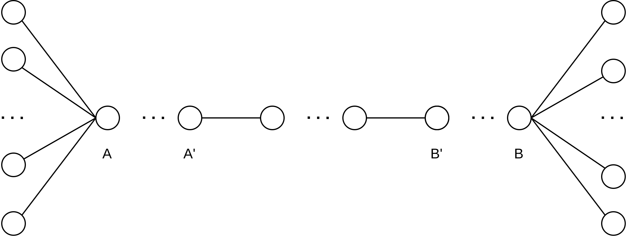
Refer to caption
Figure 4: Illustration graph for setting 2 to in the proof of Theorem 1.

(Setting 2) We proceed to the prove second bound Ω⁡(Δ​L​Dϵ2)\Omega\left(\frac{\Delta LD}{\epsilon^{2}}\right).

(Setting 2 Step 1 & Step 2) We assign all the workers with index from 11 to nn, we first define two indices set

I0=\displaystyle I_{0}= {1,⋯,|I0|},\displaystyle\left\{1,\cdots,|I_{0}|\right\}, (29)
I1=\displaystyle I_{1}= {n,n−1,⋯,n−|I1|+1}.\displaystyle\left\{n,n-1,\cdots,n-|I_{1}|+1\right\}.

where |⋅||\cdot| denotes a cardinality of a set. Consider the construction of GG in Figure 4:

If D≥n−2​⌈n/3⌉+2D\geq n-2\lceil n/3\rceil+2, then it implies the number of nodes between A and B is larger than ⌈n/3⌉\lceil n/3\rceil. In this case, denote A’ and B’ as a sub linear graph where its number of nodes is exactly ⌈n/3⌉\lceil n/3\rceil. Let all the nodes on the left of A’ be in I0I_{0} and all the nodes on the right of B’ be I1I_{1} We define all the local functions on such graph as following:

f^i​(𝒙)={−2​nn−⌈n/3⌉​Ψ​(1)​Φ​(𝒙(1))+∑i=2​k,k∈{1,2,⋯},i<T2​nn−⌈n/3⌉​[Ψ⁡(−𝒙(i))​Φ​(−𝒙(i+1))−Ψ⁡(𝒙(i))​Φ​(𝒙(i+1))]i∈I0,∑i=2​k−1,k∈{1,2,⋯},i<T2​nn−⌈n/3⌉​[Ψ⁡(−𝒙(i))​Φ​(−𝒙(i+1))−Ψ⁡(𝒙(i))​Φ​(𝒙(i+1))]i∈I1,0i∉I0,I1.\hat{f}_{i}(\boldsymbol{x})=\left\{\begin{array}[]{ll}-\frac{2n}{n-\lceil n/3\rceil}\Psi(1)\Phi(\boldsymbol{x}^{(1)})+\sum_{i=2k,k\in\{1,2,\cdots\},i<T}\frac{2n}{n-\lceil n/3\rceil}[\Psi(-\boldsymbol{x}^{(i)})\Phi(-\boldsymbol{x}^{(i+1)})-\Psi(\boldsymbol{x}^{(i)})\Phi(\boldsymbol{x}^{(i+1)})]&\quad i\in I_{0},\\ \\ \sum_{i=2k-1,k\in\{1,2,\cdots\},i<T}\frac{2n}{n-\lceil n/3\rceil}[\Psi(-\boldsymbol{x}^{(i)})\Phi(-\boldsymbol{x}^{(i+1)})-\Psi(\boldsymbol{x}^{(i)})\Phi(\boldsymbol{x}^{(i+1)})]&\quad i\in I_{1},\\ \\ 0&\quad i\not\in I_{0},I_{1}.\\ \end{array}\right. (30)

If D<n−2​⌈n/3⌉+2D<n-2\lceil n/3\rceil+2, the distance between node A and node B is D−2D-2 and the sub linear graph whose end points are A and B contains D−1D-1 nodes. We let the number of nodes on the left of AA be ⌈n−D+12⌉\left\lceil\frac{n-D+1}{2}\right\rceil, we denote the set of indices of all such nodes as I0I_{0}; and then we let the number of nodes on the right of BB be ⌊n−D+12⌋\left\lfloor\frac{n-D+1}{2}\right\rfloor, we denote the set of indices of all such nodes as III_{I}. Since D<n−2​⌈n/3⌉+2D<n-2\lceil n/3\rceil+2, this implies |I0|,|I1|>n/3|I_{0}|,|I_{1}|>n/3. We define all the local functions on such graph as following:

f^i​(𝒙)={−n|I0|​Ψ​(1)​Φ​(𝒙(1))+∑i=2​k,k∈{1,2,⋯},i<Tn|I0|​[Ψ⁡(−𝒙(i))​Φ​(−𝒙(i+1))−Ψ⁡(𝒙(i))​Φ​(𝒙(i+1))]i∈I0,∑i=2​k−1,k∈{1,2,⋯},i<Tn|I1|​[Ψ⁡(−𝒙(i))​Φ​(−𝒙(i+1))−Ψ⁡(𝒙(i))​Φ​(𝒙(i+1))]i∈I1,0i∉I0,I1.\hat{f}_{i}(\boldsymbol{x})=\left\{\begin{array}[]{ll}-\frac{n}{|I_{0}|}\Psi(1)\Phi(\boldsymbol{x}^{(1)})+\sum_{i=2k,k\in\{1,2,\cdots\},i<T}\frac{n}{|I_{0}|}[\Psi(-\boldsymbol{x}^{(i)})\Phi(-\boldsymbol{x}^{(i+1)})-\Psi(\boldsymbol{x}^{(i)})\Phi(\boldsymbol{x}^{(i+1)})]&\quad i\in I_{0},\\ \\ \sum_{i=2k-1,k\in\{1,2,\cdots\},i<T}\frac{n}{|I_{1}|}[\Psi(-\boldsymbol{x}^{(i)})\Phi(-\boldsymbol{x}^{(i+1)})-\Psi(\boldsymbol{x}^{(i)})\Phi(\boldsymbol{x}^{(i+1)})]&\quad i\in I_{1},\\ \\ 0&\quad i\not\in I_{0},I_{1}.\\ \end{array}\right. (31)

In both cases discussed based on DD, we can see that f^​(𝐱)=1n​∑i=1nf^i​(𝐱)\hat{f}(\boldsymbol{x})=\frac{1}{n}\sum_{i=1}^{n}\hat{f}_{i}(\boldsymbol{x}), and we are splitting hard zero-chain function into two main different part: the even components of the chain and the odd components of the chain. It is easy to see that for the zero chain function to make progress, it takes at least ⌈n/3⌉\lceil n/3\rceil, i.e., Ω⁡(D)\Omega(D) number of iterations in the first case (since here D=γ~​nD=\tilde{\gamma}n for some γ~>1/3\tilde{\gamma}>1/3) and DD number of iterations in the seconds case. Then the total number of iterations is lower bounded by Ω⁡(T​D)\Omega(TD).

For the oracle, we let oracle on worker ii as

[g^i​(𝒙)]j=∇jf^i​(𝒙).[\hat{g}_{i}(\boldsymbol{x})]_{j}=\nabla_{j}\hat{f}_{i}(\boldsymbol{x}). (32)

(Setting 2, Step 3) The last step is to rescale the parameters. Compared to setting 1, we know here all the f^i\hat{f}_{i} are 3​l13l_{1}-smooth, as before we let

fi​(𝒙)=L​λ23​l1​f^i​(𝒙λ),λ=6​l1​ϵL.f_{i}(\boldsymbol{x})=\frac{L\lambda^{2}}{3l_{1}}\hat{f}_{i}\left(\frac{\boldsymbol{x}}{\lambda}\right),\hskip 20.00003pt\lambda=\frac{6l_{1}\epsilon}{L}. (33)

For the Δ\Delta bound we have

L​λ2​Δ0​T/3​l1≤ΔL\lambda^{2}\Delta_{0}T/3l_{1}\leq\Delta (34)

to fulfill this it suffices to set

T=⌊Δ​LΔ0​l1​(12​ϵ)2⌋.T=\left\lfloor\frac{\Delta L}{\Delta_{0}l_{1}(12\epsilon)^{2}}\right\rfloor. (35)

It also can be seen that ff is LL-smooth. So in this setting,

Tϵ​(A,f,O,G)≥Ω⁡(T​D)=Ω⁡(Δ​L​Dϵ2).T_{\epsilon}(A,f,O,G)\geq\Omega(TD)=\Omega\left(\frac{\Delta LD}{\epsilon^{2}}\right). (36)

Combining Setting 1 and 2 we complete the proof.

Lemma 2.

In setting 1 in the proof of Theorem 1, with probability at least 1−δ1-\delta, ‖∇f​(𝐱t)‖≥ϵ\|\nabla f(\boldsymbol{x}_{t})\|\geq\epsilon for all t≤T+log⁡(δ)min⁡{n​B​p,1}​(e−1)t\leq\frac{T+\log(\delta)}{\min\{nBp,1\}(e-1)}.

Proof.

Define a filtration at iteration tt as the sigma field of all the previous events happened before iteration tt. Let ij(t)=prog​(𝐱t,j),∀j∈[n]i^{(t)}_{j}=\text{prog}(\boldsymbol{x}_{t,j}),\forall j\in[n] and i(t)=maxj⁡ij(t)i^{(t)}=\max_{j}{i^{(t)}_{j}}. And we denote ℰ(t,m,j)\mathcal{E}^{(t,m,j)} as the event of the im(t)+1i^{(t)}_{m}+1-th coordinate of output of jj-th query on worker mm at iteration tt is non-zero. Based on the independent sampling, these events are independent. Thus we know:

ℙ⁡[i(t+1)−i(t)=1|𝒰(t)]=ℙ⁡[⋃i∈[n]j≤Bℰ(t,i,j)|𝒰(t)]≤∑i∈[n],j≤Bℙ⁡[ℰ(t,i,j)|𝒰(t)]≤min⁡{n​B​p,1}.\mathbb{P}[i^{(t+1)}-i^{(t)}=1|\mathcal{U}^{(t)}]=\mathbb{P}\left[\bigcup_{\begin{subarray}{c}i\in[n]\\ j\leq B\end{subarray}}\mathcal{E}^{(t,i,j)}|\mathcal{U}^{(t)}\right]\leq\sum_{i\in[n],j\leq B}\mathbb{P}\left[\mathcal{E}^{(t,i,j)}|\mathcal{U}^{(t)}\right]\leq\min\{nBp,1\}. (37)

Let q(t)=i(t+1)−i(t)q^{(t)}=i^{(t+1)}-i^{(t)}, with Chernoff bound, we obtain

ℙ[i(t)≥T]=ℙ[e∑j=0t−1q(j)≥eT]≤e−T𝔼[e∑j=0t−1q(j)].\mathbb{P}[i^{(t)}\geq T]=\mathbb{P}[e^{\sum_{j=0}^{t-1}q^{(j)}}\geq e^{T}]\leq e^{-T}\mathbb{E}[e^{\sum_{j=0}^{t-1}q^{(j)}}]. (38)

For the expectation term we know that

𝔼⁡[e∑j=0t−1q(j)]=𝔼⁡[∏j=0t−1𝔼⁡[eq(j)|𝒰(j)]]≤(1−min⁡{n​B​p,1}+min⁡{n​B​p,1}​e)t≤emin⁡{n​B​p,1}​t​(e−1).\mathbb{E}[e^{\sum_{j=0}^{t-1}q^{(j)}}]=\mathbb{E}\left[\prod_{j=0}^{t-1}\mathbb{E}\left[e^{q^{(j)}}|\mathcal{U}^{(j)}\right]\right]\leq(1-\min\{nBp,1\}+\min\{nBp,1\}e)^{t}\leq e^{\min\{nBp,1\}t(e-1)}. (39)

Thus we know

ℙ[i(t)≥T]≤e(e−1)​min⁡{n​B​p,1}​t−T≤δ,\mathbb{P}[i^{(t)}\geq T]\leq e^{(e-1)\min\{nBp,1\}t-T}\leq\delta, (40)

for every t≤T+log⁡(δ)min⁡{n​B​p,1}​(e−1)t\leq\frac{T+\log(\delta)}{\min\{nBp,1\}(e-1)}.

B.2 Proof to Corollary 1

Proof.

Different from Theorem 3, in this corollary we do not choose DD and nn separately, so that our construction can just use the linear graph as follows:

(Linear graph, Step 1) We first let |I0|=|I1|=⌈n/3⌉|I_{0}|=|I_{1}|=\lceil n/3\rceil in the proof of Theorem 1, meaning I0I_{0} denotes the first ⌈n/3⌉\lceil n/3\rceil workers and I1I_{1} denotes the last ⌈n/3⌉\lceil n/3\rceil workers. We define all the local functions f^i​(𝐱)\hat{f}_{i}(\boldsymbol{x}) as following:

{−n⌈n/3⌉​Ψ​(1)​Φ​(𝒙(1))+∑i=2​k,k∈{1,2,⋯},i<Tn⌈n/3⌉​[Ψ⁡(−𝒙(i))​Φ​(−𝒙(i+1))−Ψ⁡(𝒙(i))​Φ​(𝒙(i+1))]i∈I0,∑i=2​k−1,k∈{1,2,⋯},i<Tn⌈n/3⌉​[Ψ⁡(−𝒙(i))​Φ​(−𝒙(i+1))−Ψ⁡(𝒙(i))​Φ​(𝒙(i+1))]i∈I1,0i∉I0,I1.\left\{\begin{array}[]{ll}-\frac{n}{\lceil n/3\rceil}\Psi(1)\Phi(\boldsymbol{x}^{(1)})+\sum_{i=2k,k\in\{1,2,\cdots\},i<T}\frac{n}{\lceil n/3\rceil}[\Psi(-\boldsymbol{x}^{(i)})\Phi(-\boldsymbol{x}^{(i+1)})-\Psi(\boldsymbol{x}^{(i)})\Phi(\boldsymbol{x}^{(i+1)})]&\quad i\in I_{0},\\ \\ \sum_{i=2k-1,k\in\{1,2,\cdots\},i<T}\frac{n}{\lceil n/3\rceil}[\Psi(-\boldsymbol{x}^{(i)})\Phi(-\boldsymbol{x}^{(i+1)})-\Psi(\boldsymbol{x}^{(i)})\Phi(\boldsymbol{x}^{(i+1)})]&\quad i\in I_{1},\\ \\ 0&\quad i\not\in I_{0},I_{1}.\\ \end{array}\right. (41)

we can see that f^​(𝐱)=1n​∑i=1nf^i​(𝐱)\hat{f}(\boldsymbol{x})=\frac{1}{n}\sum_{i=1}^{n}\hat{f}_{i}(\boldsymbol{x}). (Linear graph, Step 2) We consider linear graph in this setting and from one end to the other, the worker’s index is 11 to nn, without the loss of generality. It is easy to see that for the zero chain function to make progress, it takes at least n−2​⌈n/3⌉+1n-2\lceil n/3\rceil+1 number of iterations. Note that in linear graph n−1=Dn-1=D, the total number of iterations is at least

Ω⁡(T​D).\Omega\left(TD\right). (42)

For the oracle, we let oracle on worker ii as

[g^i​(𝒙)]j=∇jf^i​(𝒙)[\hat{g}_{i}(\boldsymbol{x})]_{j}=\nabla_{j}\hat{f}_{i}(\boldsymbol{x}) (43)

(Linear graph, Step 3) The last step is to rescale the parameters. Compared to setting 1, we know here all the f^i\hat{f}_{i} are 3​l13l_{1}-smooth, as before we let

fi​(𝒙)=L​λ23​l1​f^i​(𝒙λ),λ=6​l1​ϵL.f_{i}(\boldsymbol{x})=\frac{L\lambda^{2}}{3l_{1}}\hat{f}_{i}\left(\frac{\boldsymbol{x}}{\lambda}\right),\hskip 20.00003pt\lambda=\frac{6l_{1}\epsilon}{L}. (44)

For the Δ\Delta bound we have

L​λ2​Δ0​T/3​l1≤Δ,L\lambda^{2}\Delta_{0}T/3l_{1}\leq\Delta, (45)

to fulfill this it suffices to set

T=⌊Δ​LΔ0​l1​(12​ϵ)2⌋.T=\left\lfloor\frac{\Delta L}{\Delta_{0}l_{1}(12\epsilon)^{2}}\right\rfloor. (46)

It also can be seen that ff is LL-smooth. So in this setting,

Tϵ​(A,f,O,G)≥Ω⁡(T​D)≥Ω⁡(Δ​L​Dϵ2).T_{\epsilon}(A,f,O,G)\geq\Omega(TD)\geq\Omega\left(\frac{\Delta LD}{\epsilon^{2}}\right). (47)

Given the bound, we use two additional results on linear graph as [86]: the random walk matrix 𝐖r​w\boldsymbol{W}_{rw} on linear graph with λ\lambda fulfilling

11−λ=O⁡(D).\displaystyle\frac{1}{\sqrt{1-\lambda}}=O(D). (48)

Then we can rewrite the lower bound in the form of λ\lambda as shown in Corollary 1.

Finally, using the conclusion of λ=cos⁡(π/n)\lambda=\cos(\pi/n) for n∈{2,3,⋯,}n\in\{2,3,\cdots,\} on linear graph we complete the proof.

B.3 Proof to Theorem 2

Proof.

As (partially) discussed in the paper, DeFacto is statistically equivalent to centralized SGD. Specifically, it conduct K=T/2​RK=T/2R gradient steps where each step contains a mini-batch of RR at the point of 𝐱k,i,∀i∈[n]\boldsymbol{x}_{k,i},\forall i\in[n]. Take the well-known convergence rate for centralized SGD:

1T​∑t=0T−1‖∇f​(𝒙^)‖2≤O⁡(Δ​L​σn​B​T+Δ​LT).\frac{1}{T}\sum_{t=0}^{T-1}\|\nabla f(\boldsymbol{\hat{x}})\|^{2}\leq O\left(\frac{\Delta L\sigma}{\sqrt{nBT}}+\frac{\Delta L}{T}\right). (49)

The convergence rate of DeFacto can be expressed as:

1T​∑t=0T−1‖∇f​(𝒙^)‖2≤O⁡(Δ​L​σ/Rn​B​K+Δ​LK)=O⁡(Δ​L​σn​B​T+Δ​L​RT)=O⁡(Δ​L​σn​B​T+Δ​L​DT),\frac{1}{T}\sum_{t=0}^{T-1}\|\nabla f(\boldsymbol{\hat{x}})\|^{2}\leq O\left(\frac{\Delta L\sigma/\sqrt{R}}{\sqrt{nBK}}+\frac{\Delta L}{K}\right)=O\left(\frac{\Delta L\sigma}{\sqrt{nBT}}+\frac{\Delta LR}{T}\right)=O\left(\frac{\Delta L\sigma}{\sqrt{nBT}}+\frac{\Delta LD}{T}\right), (50)

then we obtain for DeFacto, when T=O⁡(Δ​L​σ2​(n​B​ϵ4)−1+Δ​L​D​ϵ−2)T=O(\Delta L\sigma^{2}(nB\epsilon^{4})^{-1}+\Delta LD\epsilon^{-2}),

mint=0,1,⋯,T−1⁡𝔼⁡‖∇f​(𝒙^)‖≤mint=0,1,⋯,T−1⁡𝔼​‖∇f​(𝒙^)‖2≤O⁡(Δ​L​σn​B​T+Δ​L​DT)≤ϵ,\min_{t=0,1,\cdots,T-1}\mathbb{E}\left\|\nabla f\left(\boldsymbol{\hat{x}}\right)\right\|\leq\sqrt{\min_{t=0,1,\cdots,T-1}\mathbb{E}\left\|\nabla f\left(\boldsymbol{\hat{x}}\right)\right\|^{2}}\leq\sqrt{O\left(\frac{\Delta L\sigma}{\sqrt{nBT}}+\frac{\Delta LD}{T}\right)}\leq\epsilon, (51)

that completes the proof.

B.4 Proof to Theorem 3

Proof.

In this proof, we adopt an updated version of notation: we denote at the beginning of phase kk, the three quantities of interests are 𝐗k\boldsymbol{X}_{k}, 𝐘k\boldsymbol{Y}_{k} and 𝐆~k\tilde{\boldsymbol{G}}_{k}, and the update rule becomes:

𝒀k+1=ℳ⁡(𝒀k+𝑮~k−𝑮~k−1),\displaystyle\boldsymbol{Y}_{k+1}=\mathcal{M}(\boldsymbol{Y}_{k}+\tilde{\boldsymbol{G}}_{k}-\tilde{\boldsymbol{G}}_{k-1}), (52)
𝑿k+1=ℳ⁡(𝑿k−α​𝒀k),\displaystyle\boldsymbol{X}_{k+1}=\mathcal{M}(\boldsymbol{X}_{k}-\alpha\boldsymbol{Y}_{k}), (53)

with

𝑮~k+1=\displaystyle\tilde{\boldsymbol{G}}_{k+1}= [∇f~1​(𝒙k,1),⋯,∇f~n​(𝒙k,n)]∈ℝd×n,\displaystyle\left[\nabla\tilde{f}_{1}(\boldsymbol{x}_{k,1}),\cdots,\nabla\tilde{f}_{n}(\boldsymbol{x}_{k,n})\right]\in\mathbb{R}^{d\times n}, (54)
𝑮k+1=\displaystyle\boldsymbol{G}_{k+1}= [∇f1​(𝒙k,1),⋯,∇fn​(𝒙k,n)]∈ℝd×n,\displaystyle\left[\nabla f_{1}(\boldsymbol{x}_{k,1}),\cdots,\nabla f_{n}(\boldsymbol{x}_{k,n})\right]\in\mathbb{R}^{d\times n}, (55)
𝑿k=\displaystyle{\boldsymbol{X}}_{k}= [𝒙k,1,⋯,𝒙k,n]∈ℝd×n,\displaystyle\left[\boldsymbol{x}_{k,1},\cdots,\boldsymbol{x}_{k,n}\right]\in\mathbb{R}^{d\times n}, (56)
𝒀k=\displaystyle{\boldsymbol{Y}}_{k}= [𝒚k,1,⋯,𝒚k,n]∈ℝd×n,\displaystyle\left[\boldsymbol{y}_{k,1},\cdots,\boldsymbol{y}_{k,n}\right]\in\mathbb{R}^{d\times n}, (57)

where ∇f~i\nabla\tilde{f}_{i} denotes the stochastic gradient oracle on worker ii, and ∇fi\nabla f_{i} denotes the full gradient oracle on worker ii. We use 𝐗¯\overline{\boldsymbol{X}} denote 𝐗​𝟏n\boldsymbol{X}\frac{\boldsymbol{1}}{n} for any matrix 𝐗\boldsymbol{X} with appropriate shape. We use λi​(𝐖)\lambda_{i}(\boldsymbol{W}) to denote the ii-th general largest eigenvalue of matrix 𝐖\boldsymbol{W}. Under such notation, λ\lambda in the main paper is equavilent to λ2​(𝐖)\lambda_{2}(\boldsymbol{W}). We use ℳ⁡(⋅)\mathcal{M}(\cdot) to denote the RR-step accelerated gossip which has the following property [87]:

‖ℳ⁡(𝑿)−𝑿¯‖≤ρ​‖𝑿−𝑿¯‖;ℳ⁡(𝑿)​𝟏n=𝑿​𝟏n,\displaystyle\|\mathcal{M}(\boldsymbol{X})-\overline{\boldsymbol{X}}\|\leq\rho\|\boldsymbol{X}-\overline{\boldsymbol{X}}\|;\hskip 10.00002pt\mathcal{M}(\boldsymbol{X})\frac{\boldsymbol{1}}{n}=\boldsymbol{X}\frac{\boldsymbol{1}}{n}, (58)

where ρ=(1−1−λ2​(𝐖))R\rho=\left(1-\sqrt{1-\lambda_{2}(\boldsymbol{W})}\right)^{R}. The proof to the statement of Equation (58) can be found in [88].

For the stochastic oracle, based on the oracle class assumption, we have

𝔼​‖∇f~i​(𝒙)−∇fi​(𝒙)‖2≤σ2,\displaystyle\mathbb{E}\|\nabla\tilde{f}_{i}(\boldsymbol{x})-\nabla f_{i}(\boldsymbol{x})\|^{2}\leq\sigma^{2}, (59)

and we denote σ~2=σ2B​R\tilde{\sigma}^{2}=\frac{\sigma^{2}}{BR} as the variance of mini-batch of RR.

First, from the update rule of DeTAG,

𝒀¯k=ℳ⁡(𝒀k−1+𝑮~k−1−𝑮~k−2)​𝟏n=𝒀¯k−1+𝑮~¯k−1−𝑮~¯k−2=𝒀¯−1+∑j=−1k−1(𝑮~¯j−𝑮~¯j−1)=𝑮~¯k−1\overline{\boldsymbol{Y}}_{k}=\mathcal{M}(\boldsymbol{Y}_{k-1}+\tilde{\boldsymbol{G}}_{k-1}-\tilde{\boldsymbol{G}}_{k-2})\frac{\boldsymbol{1}}{n}=\overline{\boldsymbol{Y}}_{k-1}+\overline{\tilde{\boldsymbol{G}}}_{k-1}-\overline{\tilde{\boldsymbol{G}}}_{k-2}=\overline{\boldsymbol{Y}}_{-1}+\sum_{j=-1}^{k-1}(\overline{\tilde{\boldsymbol{G}}}_{j}-\overline{\tilde{\boldsymbol{G}}}_{j-1})=\overline{\tilde{\boldsymbol{G}}}_{k-1} (60)

and

𝑿¯k+1=ℳ⁡(𝑿k−α​𝒀k)​𝟏n=𝑿¯k−α​𝒀¯k.\overline{\boldsymbol{X}}_{k+1}=\mathcal{M}(\boldsymbol{X}_{k}-\alpha\boldsymbol{Y}_{k})\frac{\boldsymbol{1}}{n}=\overline{\boldsymbol{X}}_{k}-\alpha\overline{\boldsymbol{Y}}_{k}. (61)

By Taylor Theorem, we obtain

𝔼​f​(𝑿¯k+1)=\displaystyle\mathbb{E}f\left(\overline{\boldsymbol{X}}_{k+1}\right)= 𝔼​f​(𝑿¯k−α​𝒀¯k)\displaystyle\mathbb{E}f\left(\overline{\boldsymbol{X}}_{k}-\alpha\overline{\boldsymbol{Y}}_{k}\right) (62)
≤\displaystyle\leq 𝔼​f​(𝑿¯k)−α​𝔼​⟨∇f​(𝑿¯k),𝒀¯k⟩+α2​L2​𝔼​‖𝒀¯k‖2\displaystyle\mathbb{E}f\left(\overline{\boldsymbol{X}}_{k}\right)-\alpha\mathbb{E}\left\langle\nabla f\left(\overline{\boldsymbol{X}}_{k}\right),\overline{\boldsymbol{Y}}_{k}\right\rangle+\frac{\alpha^{2}L}{2}\mathbb{E}\left\|\overline{\boldsymbol{Y}}_{k}\right\|^{2} (63)
=(60)\displaystyle\overset{(\ref{proof equation Yk})}{=} 𝔼​f​(𝑿¯k)−α​𝔼​⟨∇f​(𝑿¯k),𝑮¯k−1⟩+α2​L2​𝔼​‖𝑮~¯k−1‖2.\displaystyle\mathbb{E}f\left(\overline{\boldsymbol{X}}_{k}\right)-\alpha\mathbb{E}\left\langle\nabla f\left(\overline{\boldsymbol{X}}_{k}\right),\overline{\boldsymbol{G}}_{k-1}\right\rangle+\frac{\alpha^{2}L}{2}\mathbb{E}\left\|\overline{\tilde{\boldsymbol{G}}}_{k-1}\right\|^{2}. (64)

For the last term, we have

𝔼​‖𝑮~¯k−1‖2=\displaystyle\mathbb{E}\left\|\overline{\tilde{\boldsymbol{G}}}_{k-1}\right\|^{2}= 𝔼​‖𝑮¯k−1‖2+𝔼​‖𝑮¯k−1−𝑮~¯k−1‖2+2​𝔼​⟨𝑮¯k−1,𝑮¯k−1−𝑮~¯k−1⟩\displaystyle\mathbb{E}\left\|\overline{\boldsymbol{G}}_{k-1}\right\|^{2}+\mathbb{E}\left\|\overline{\boldsymbol{G}}_{k-1}-\overline{\tilde{\boldsymbol{G}}}_{k-1}\right\|^{2}+2\mathbb{E}\left\langle\overline{\boldsymbol{G}}_{k-1},\overline{\boldsymbol{G}}_{k-1}-\overline{\tilde{\boldsymbol{G}}}_{k-1}\right\rangle (65)
=\displaystyle= 𝔼​‖𝑮¯k−1‖2+𝔼​‖𝑮¯k−1−𝑮~¯k−1‖2\displaystyle\mathbb{E}\left\|\overline{\boldsymbol{G}}_{k-1}\right\|^{2}+\mathbb{E}\left\|\overline{\boldsymbol{G}}_{k-1}-\overline{\tilde{\boldsymbol{G}}}_{k-1}\right\|^{2} (66)
=\displaystyle= 𝔼​‖𝑮¯k−1‖2+1n2​∑i=1n𝔼​‖𝑮k−1​𝒆i−𝑮~k−1​𝒆i‖2\displaystyle\mathbb{E}\left\|\overline{\boldsymbol{G}}_{k-1}\right\|^{2}+\frac{1}{n^{2}}\sum_{i=1}^{n}\mathbb{E}\left\|\boldsymbol{G}_{k-1}\boldsymbol{e}_{i}-\boldsymbol{\tilde{G}}_{k-1}\boldsymbol{e}_{i}\right\|^{2} (67)
≤\displaystyle\leq 𝔼​‖𝑮¯k−1‖2+σ~2n,\displaystyle\mathbb{E}\left\|\overline{\boldsymbol{G}}_{k-1}\right\|^{2}+\frac{\tilde{\sigma}^{2}}{n}, (68)

where in the second step, we use the fact that the sampling noise is independent of the gradient itself. Putting it back we obtain

𝔼​f​(𝑿¯k+1)≤\displaystyle\mathbb{E}f\left(\overline{\boldsymbol{X}}_{k+1}\right)\leq 𝔼​f​(𝑿¯k)−α​𝔼​⟨∇f​(𝑿¯k),𝑮¯k−1⟩+α2​L2​𝔼​‖𝑮¯k−1‖2+α2​σ~2​L2​n\displaystyle\mathbb{E}f\left(\overline{\boldsymbol{X}}_{k}\right)-\alpha\mathbb{E}\left\langle\nabla f\left(\overline{\boldsymbol{X}}_{k}\right),\overline{\boldsymbol{G}}_{k-1}\right\rangle+\frac{\alpha^{2}L}{2}\mathbb{E}\left\|\overline{\boldsymbol{G}}_{k-1}\right\|^{2}+\frac{\alpha^{2}\tilde{\sigma}^{2}L}{2n} (69)
=\displaystyle= 𝔼​f​(𝑿¯k)−α2​𝔼​‖∇f​(𝑿¯k)‖2−α−α2​L2​‖𝑮¯k−1‖2+α2​σ~2​L2​n+α2​𝔼​‖𝑮¯k−1−∇f​(𝑿¯k)‖2,\displaystyle\mathbb{E}f\left(\overline{\boldsymbol{X}}_{k}\right)-\frac{\alpha}{2}\mathbb{E}\left\|\nabla f\left(\overline{\boldsymbol{X}}_{k}\right)\right\|^{2}-\frac{\alpha-\alpha^{2}L}{2}\left\|\overline{\boldsymbol{G}}_{k-1}\right\|^{2}+\frac{\alpha^{2}\tilde{\sigma}^{2}L}{2n}+\frac{\alpha}{2}\mathbb{E}\left\|\overline{\boldsymbol{G}}_{k-1}-\nabla f\left(\overline{\boldsymbol{X}}_{k}\right)\right\|^{2}, (70)

where the last step we use 2​⟨a,b⟩=‖a‖2+‖b‖2−‖a−b‖22\langle a,b\rangle=\|a\|^{2}+\|b\|^{2}-\|a-b\|^{2}. Expand the last term, we obtain

𝔼​‖𝑮¯k−1−∇f​(𝑿¯k)‖2\displaystyle\mathbb{E}\left\|\overline{\boldsymbol{G}}_{k-1}-\nabla f\left(\overline{\boldsymbol{X}}_{k}\right)\right\|^{2} (71)
≤\displaystyle\leq 2​𝔼​‖𝑮¯k−1−𝑮¯k+1‖2+2​𝔼​‖𝑮¯k+1−∇f​(𝑿¯k)‖2\displaystyle 2\mathbb{E}\left\|\overline{\boldsymbol{G}}_{k-1}-\overline{\boldsymbol{G}}_{k+1}\right\|^{2}+2\mathbb{E}\left\|\overline{\boldsymbol{G}}_{k+1}-\nabla f\left(\overline{\boldsymbol{X}}_{k}\right)\right\|^{2} (72)
=\displaystyle= 2​𝔼​‖1n​∑i=1n∇fi​(𝒙k,i)−1n​∑i=1n∇fi​(𝒙k−2,i)‖2+2​𝔼​‖1n​∑i=1n∇fi​(𝒙k,i)−1n​∑i=1n∇fi​(𝑿¯k)‖2\displaystyle 2\mathbb{E}\left\|\frac{1}{n}\sum_{i=1}^{n}\nabla f_{i}(\boldsymbol{x}_{k,i})-\frac{1}{n}\sum_{i=1}^{n}\nabla f_{i}(\boldsymbol{x}_{k-2,i})\right\|^{2}+2\mathbb{E}\left\|\frac{1}{n}\sum_{i=1}^{n}\nabla f_{i}(\boldsymbol{x}_{k,i})-\frac{1}{n}\sum_{i=1}^{n}\nabla f_{i}(\overline{\boldsymbol{X}}_{k})\right\|^{2} (73)
≤\displaystyle\leq 2n​∑i=1n𝔼​‖∇fi​(𝒙k,i)−∇fi​(𝒙k−2,i)‖2+2n​∑i=1n𝔼​‖∇fi​(𝒙k,i)−∇fi​(𝑿¯k)‖2\displaystyle\frac{2}{n}\sum_{i=1}^{n}\mathbb{E}\left\|\nabla f_{i}(\boldsymbol{x}_{k,i})-\nabla f_{i}(\boldsymbol{x}_{k-2,i})\right\|^{2}+\frac{2}{n}\sum_{i=1}^{n}\mathbb{E}\left\|\nabla f_{i}(\boldsymbol{x}_{k,i})-\nabla f_{i}(\overline{\boldsymbol{X}}_{k})\right\|^{2} (74)
≤\displaystyle\leq 2​L2n​𝔼​‖𝑿k−𝑿k−2‖F2+2​L2n​𝔼​‖𝑿k−𝑿¯k​𝟏n⊤‖F2.\displaystyle\frac{2L^{2}}{n}\mathbb{E}\left\|\boldsymbol{X}_{k}-\boldsymbol{X}_{k-2}\right\|_{F}^{2}+\frac{2L^{2}}{n}\mathbb{E}\left\|\boldsymbol{X}_{k}-\overline{\boldsymbol{X}}_{k}\boldsymbol{1}_{n}^{\top}\right\|_{F}^{2}. (75)

Denote f⁡(𝟎)−f∗≤Δf(\boldsymbol{0})-f^{*}\leq\Delta, we obtain

∑k=0K−1α⁡(1−α​L)​‖𝑮¯k‖2+∑k=0K−1α​𝔼​‖∇f​(𝑿¯k)‖2\displaystyle\sum_{k=0}^{K-1}\alpha(1-\alpha L)\left\|\overline{\boldsymbol{G}}_{k}\right\|^{2}+\sum_{k=0}^{K-1}\alpha\mathbb{E}\left\|\nabla f\left(\overline{\boldsymbol{X}}_{k}\right)\right\|^{2} (76)
≤\displaystyle\leq 2​Δ+α2​σ~2​L​Kn+2​α​L2n​∑k=0K−1𝔼​‖𝑿k−𝑿¯k​𝟏n⊤‖F2+2​α​L2n​∑k=0K−1𝔼​‖𝑿k−𝑿k−2‖F2\displaystyle 2\Delta+\frac{\alpha^{2}\tilde{\sigma}^{2}LK}{n}+\frac{2\alpha L^{2}}{n}\sum_{k=0}^{K-1}\mathbb{E}\left\|\boldsymbol{X}_{k}-\overline{\boldsymbol{X}}_{k}\boldsymbol{1}_{n}^{\top}\right\|_{F}^{2}+\frac{2\alpha L^{2}}{n}\sum_{k=0}^{K-1}\mathbb{E}\left\|\boldsymbol{X}_{k}-\boldsymbol{X}_{k-2}\right\|_{F}^{2} (77)
≤\displaystyle\leq 2​Δ+α2​σ~2​L​Kn+16​α​L2n​∑k=0K−1𝔼​‖𝑿k−𝑿¯k​𝟏n⊤‖F2+6​α​L2n​∑k=0K−1𝔼​‖𝑿¯k​𝟏n⊤−𝑿¯k−2​𝟏n⊤‖F2,\displaystyle 2\Delta+\frac{\alpha^{2}\tilde{\sigma}^{2}LK}{n}+\frac{16\alpha L^{2}}{n}\sum_{k=0}^{K-1}\mathbb{E}\left\|\boldsymbol{X}_{k}-\overline{\boldsymbol{X}}_{k}\boldsymbol{1}_{n}^{\top}\right\|_{F}^{2}+\frac{6\alpha L^{2}}{n}\sum_{k=0}^{K-1}\mathbb{E}\left\|\overline{\boldsymbol{X}}_{k}\boldsymbol{1}_{n}^{\top}-\overline{\boldsymbol{X}}_{k-2}\boldsymbol{1}_{n}^{\top}\right\|_{F}^{2}, (78)

where in the last step we use

2​α​L2n​∑k=0K−1𝔼​‖𝑿k−𝑿k−2‖F2\displaystyle\frac{2\alpha L^{2}}{n}\sum_{k=0}^{K-1}\mathbb{E}\left\|\boldsymbol{X}_{k}-\boldsymbol{X}_{k-2}\right\|_{F}^{2} (79)
≤\displaystyle\leq 6​α​L2n​∑k=0K−1𝔼​‖𝑿k−𝑿¯k​𝟏n⊤‖F2+6​α​L2n​∑k=0K−1𝔼​‖𝑿k−2−𝑿¯k−2​𝟏n⊤‖F2+6​α​L2n​∑k=0K−1𝔼​‖𝑿¯k​𝟏n⊤−𝑿¯k−2​𝟏n⊤‖F2.\displaystyle\frac{6\alpha L^{2}}{n}\sum_{k=0}^{K-1}\mathbb{E}\left\|\boldsymbol{X}_{k}-\overline{\boldsymbol{X}}_{k}\boldsymbol{1}_{n}^{\top}\right\|_{F}^{2}+\frac{6\alpha L^{2}}{n}\sum_{k=0}^{K-1}\mathbb{E}\left\|\boldsymbol{X}_{k-2}-\overline{\boldsymbol{X}}_{k-2}\boldsymbol{1}_{n}^{\top}\right\|_{F}^{2}+\frac{6\alpha L^{2}}{n}\sum_{k=0}^{K-1}\mathbb{E}\left\|\overline{\boldsymbol{X}}_{k}\boldsymbol{1}_{n}^{\top}-\overline{\boldsymbol{X}}_{k-2}\boldsymbol{1}_{n}^{\top}\right\|_{F}^{2}. (80)

In addition, for the last term we have

6​α​L2n​∑k=0K−1𝔼​‖𝑿¯k​𝟏n⊤−𝑿¯k−2​𝟏n⊤‖F2=\displaystyle\frac{6\alpha L^{2}}{n}\sum_{k=0}^{K-1}\mathbb{E}\left\|\overline{\boldsymbol{X}}_{k}\boldsymbol{1}_{n}^{\top}-\overline{\boldsymbol{X}}_{k-2}\boldsymbol{1}_{n}^{\top}\right\|_{F}^{2}= 6​α​L2​nn​∑k=0K−1𝔼​‖𝑿¯k−𝑿¯k−2‖2\displaystyle\frac{6\alpha L^{2}n}{n}\sum_{k=0}^{K-1}\mathbb{E}\left\|\overline{\boldsymbol{X}}_{k}-\overline{\boldsymbol{X}}_{k-2}\right\|^{2} (81)
=(61)\displaystyle\overset{(\ref{proof equation Xk})}{=} 24​α3​L2​nn​∑k=0K−1𝔼​‖𝑮~¯k‖2\displaystyle\frac{24\alpha^{3}L^{2}n}{n}\sum_{k=0}^{K-1}\mathbb{E}\left\|\overline{\tilde{\boldsymbol{G}}}_{k}\right\|^{2} (82)
≤(65)\displaystyle\overset{(\ref{proof equation sampling noise})}{\leq} 24​α3​L2​∑k=0K−1𝔼​‖𝑮¯k‖2+24​α3​σ~2​L2​Kn.\displaystyle 24\alpha^{3}L^{2}\sum_{k=0}^{K-1}\mathbb{E}\left\|\overline{{\boldsymbol{G}}}_{k}\right\|^{2}+\frac{24\alpha^{3}\tilde{\sigma}^{2}L^{2}K}{n}. (83)

Push it back we have

∑k=0K−1α⁡(1−α​L−24​α2​L2)​‖𝑮¯k‖2+∑k=0K−1α​𝔼​‖∇f​(𝑿¯k)‖2\displaystyle\sum_{k=0}^{K-1}\alpha(1-\alpha L-24\alpha^{2}L^{2})\left\|\overline{\boldsymbol{G}}_{k}\right\|^{2}+\sum_{k=0}^{K-1}\alpha\mathbb{E}\left\|\nabla f\left(\overline{\boldsymbol{X}}_{k}\right)\right\|^{2} (84)
≤\displaystyle\leq 2​Δ+α2​σ~2​L​Kn+16​α​L2n​∑k=0K−1𝔼​‖𝑿k−𝑿¯k​𝟏n⊤‖F2+24​α3​σ~2​L2​Kn.\displaystyle 2\Delta+\frac{\alpha^{2}\tilde{\sigma}^{2}LK}{n}+\frac{16\alpha L^{2}}{n}\sum_{k=0}^{K-1}\mathbb{E}\left\|\boldsymbol{X}_{k}-\overline{\boldsymbol{X}}_{k}\boldsymbol{1}_{n}^{\top}\right\|_{F}^{2}+\frac{24\alpha^{3}\tilde{\sigma}^{2}L^{2}K}{n}. (85)

The rest of the proof is to bound 16​α​L2n​∑k=0K−1𝔼​‖𝐗k−𝐗¯k​𝟏n⊤‖F2\frac{16\alpha L^{2}}{n}\sum_{k=0}^{K-1}\mathbb{E}\left\|\boldsymbol{X}_{k}-\overline{\boldsymbol{X}}_{k}\boldsymbol{1}_{n}^{\top}\right\|_{F}^{2}.

We start from

‖𝑿k+1−𝑿¯k+1​𝟏n⊤‖F2\displaystyle\left\|\boldsymbol{X}_{k+1}-\overline{\boldsymbol{X}}_{k+1}\boldsymbol{1}_{n}^{\top}\right\|_{F}^{2} (86)
=(61)\displaystyle\overset{(\ref{proof equation Xk})}{=} ‖ℳ⁡(𝑿k−α​𝒀k)−(𝑿¯k−α​𝒀¯k)​𝟏n⊤‖F2\displaystyle\left\|\mathcal{M}(\boldsymbol{X}_{k}-\alpha\boldsymbol{Y}_{k})-(\overline{\boldsymbol{X}}_{k}-\alpha\overline{\boldsymbol{Y}}_{k})\boldsymbol{1}_{n}^{\top}\right\|_{F}^{2} (87)
=\displaystyle= ‖ℳ⁡(𝑿k)−𝑿¯k​𝟏n⊤‖F2−2​α​⟨ℳ⁡(𝑿k)−𝑿¯k​𝟏n⊤,ℳ⁡(𝒀k)−𝒀¯k​𝟏n⊤⟩+α2​‖ℳ⁡(𝒀k)−𝒀¯k​𝟏n⊤‖F2\displaystyle\left\|\mathcal{M}(\boldsymbol{X}_{k})-\overline{\boldsymbol{X}}_{k}\boldsymbol{1}_{n}^{\top}\right\|_{F}^{2}-2\alpha\left\langle\mathcal{M}(\boldsymbol{X}_{k})-\overline{\boldsymbol{X}}_{k}\boldsymbol{1}_{n}^{\top},\mathcal{M}(\boldsymbol{Y}_{k})-\overline{\boldsymbol{Y}}_{k}\boldsymbol{1}_{n}^{\top}\right\rangle+\alpha^{2}\left\|\mathcal{M}(\boldsymbol{Y}_{k})-\overline{\boldsymbol{Y}}_{k}\boldsymbol{1}_{n}^{\top}\right\|_{F}^{2} (88)
≤(58)\displaystyle\overset{(\ref{proof equation property AG})}{\leq} ρ2​‖𝑿k−𝑿¯k​𝟏n⊤‖F2+ρ2​(1−ρ2)1+ρ2​‖𝑿k−𝑿¯k​𝟏n⊤‖F2+ρ2​(1+ρ2)​α21−ρ2​‖𝒀k−𝒀¯k​𝟏n⊤‖F2\displaystyle\rho^{2}\left\|\boldsymbol{X}_{k}-\overline{\boldsymbol{X}}_{k}\boldsymbol{1}_{n}^{\top}\right\|_{F}^{2}+\frac{\rho^{2}(1-\rho^{2})}{1+\rho^{2}}\left\|\boldsymbol{X}_{k}-\overline{\boldsymbol{X}}_{k}\boldsymbol{1}_{n}^{\top}\right\|_{F}^{2}+\frac{\rho^{2}(1+\rho^{2})\alpha^{2}}{1-\rho^{2}}\left\|\boldsymbol{Y}_{k}-\overline{\boldsymbol{Y}}_{k}\boldsymbol{1}_{n}^{\top}\right\|_{F}^{2} (89)
+α2​ρ2​‖𝒀k−𝒀¯k​𝟏n⊤‖F2\displaystyle+\alpha^{2}\rho^{2}\left\|\boldsymbol{Y}_{k}-\overline{\boldsymbol{Y}}_{k}\boldsymbol{1}_{n}^{\top}\right\|_{F}^{2} (90)
=\displaystyle= 2​ρ2(1+ρ2)​‖𝑿k−𝑿¯k​𝟏n⊤‖F2+2​ρ2​α21−ρ2​‖𝒀k−𝒀¯k​𝟏n⊤‖F2,\displaystyle\frac{2\rho^{2}}{(1+\rho^{2})}\left\|\boldsymbol{X}_{k}-\overline{\boldsymbol{X}}_{k}\boldsymbol{1}_{n}^{\top}\right\|_{F}^{2}+\frac{2\rho^{2}\alpha^{2}}{1-\rho^{2}}\left\|\boldsymbol{Y}_{k}-\overline{\boldsymbol{Y}}_{k}\boldsymbol{1}_{n}^{\top}\right\|_{F}^{2}, (91)

where in the third step we use

−2​⟨𝒂,𝒃⟩≤1−ρ21+ρ2​‖𝒂‖2+1+ρ21−ρ2​‖𝒃‖2.\displaystyle-2\langle\boldsymbol{a},\boldsymbol{b}\rangle\leq\frac{1-\rho^{2}}{1+\rho^{2}}\|\boldsymbol{a}\|^{2}+\frac{1+\rho^{2}}{1-\rho^{2}}\|\boldsymbol{b}\|^{2}. (92)

Similarly, for 𝐘k+1\boldsymbol{Y}_{k+1}, we obtain

𝔼​‖𝒀k+1−𝒀¯k+1​𝟏n⊤‖F2\displaystyle\mathbb{E}\left\|\boldsymbol{Y}_{k+1}-\overline{\boldsymbol{Y}}_{k+1}\boldsymbol{1}_{n}^{\top}\right\|_{F}^{2} (93)
=(60)\displaystyle\overset{(\ref{proof equation Yk})}{=} 𝔼​‖ℳ⁡(𝒀k+𝑮~k−𝑮~k−1)−(𝒀¯k+𝑮~¯k−𝑮~¯k−1)​𝟏n⊤‖F2\displaystyle\mathbb{E}\left\|\mathcal{M}(\boldsymbol{Y}_{k}+\tilde{\boldsymbol{G}}_{k}-\tilde{\boldsymbol{G}}_{k-1})-(\overline{\boldsymbol{Y}}_{k}+\overline{\tilde{\boldsymbol{G}}}_{k}-\overline{\tilde{\boldsymbol{G}}}_{k-1})\boldsymbol{1}_{n}^{\top}\right\|_{F}^{2} (94)
=\displaystyle= 𝔼​‖ℳ⁡(𝒀k)−𝒀¯k​𝟏n⊤‖F2+𝔼​‖ℳ⁡(𝑮~k−𝑮~k−1)−(𝑮~¯k−𝑮~¯k−1)​𝟏n⊤‖F2\displaystyle\mathbb{E}\left\|\mathcal{M}(\boldsymbol{Y}_{k})-\overline{\boldsymbol{Y}}_{k}\boldsymbol{1}_{n}^{\top}\right\|_{F}^{2}+\mathbb{E}\left\|\mathcal{M}(\tilde{\boldsymbol{G}}_{k}-\tilde{\boldsymbol{G}}_{k-1})-(\overline{\tilde{\boldsymbol{G}}}_{k}-\overline{\tilde{\boldsymbol{G}}}_{k-1})\boldsymbol{1}_{n}^{\top}\right\|_{F}^{2} (95)
+2​𝔼​⟨ℳ⁡(𝒀k)−𝒀¯k​𝟏n⊤,ℳ⁡(𝑮~k−𝑮~k−1)−(𝑮~¯k−𝑮~¯k−1)​𝟏n⊤⟩\displaystyle+2\mathbb{E}\left\langle\mathcal{M}(\boldsymbol{Y}_{k})-\overline{\boldsymbol{Y}}_{k}\boldsymbol{1}_{n}^{\top},\mathcal{M}(\tilde{\boldsymbol{G}}_{k}-\tilde{\boldsymbol{G}}_{k-1})-(\overline{\tilde{\boldsymbol{G}}}_{k}-\overline{\tilde{\boldsymbol{G}}}_{k-1})\boldsymbol{1}_{n}^{\top}\right\rangle (96)
≤(92)​(58)\displaystyle\overset{(\ref{proof equation square trick})(\ref{proof equation property AG})}{\leq} ρ2​𝔼​‖𝒀k−𝒀¯k​𝟏n⊤‖F2+ρ2​𝔼​‖𝑮k−𝑮k−1−(𝑮¯k−𝑮¯k−1)​𝟏n⊤‖F2\displaystyle\rho^{2}\mathbb{E}\left\|\boldsymbol{Y}_{k}-\overline{\boldsymbol{Y}}_{k}\boldsymbol{1}_{n}^{\top}\right\|_{F}^{2}+\rho^{2}\mathbb{E}\left\|\boldsymbol{G}_{k}-\boldsymbol{G}_{k-1}-(\overline{\boldsymbol{G}}_{k}-\overline{\boldsymbol{G}}_{k-1})\boldsymbol{1}_{n}^{\top}\right\|_{F}^{2} (97)
+(1−ρ2)​ρ21+ρ2​𝔼​‖𝒀k−𝒀¯k​𝟏n⊤‖F2+(1+ρ2)​ρ21−ρ2​𝔼​‖𝑮k−𝑮k−1−(𝑮¯k−𝑮¯k−1)​𝟏n⊤‖F2\displaystyle+\frac{(1-\rho^{2})\rho^{2}}{1+\rho^{2}}\mathbb{E}\left\|\boldsymbol{Y}_{k}-\overline{\boldsymbol{Y}}_{k}\boldsymbol{1}_{n}^{\top}\right\|_{F}^{2}+\frac{(1+\rho^{2})\rho^{2}}{1-\rho^{2}}\mathbb{E}\left\|\boldsymbol{G}_{k}-\boldsymbol{G}_{k-1}-(\overline{\boldsymbol{G}}_{k}-\overline{\boldsymbol{G}}_{k-1})\boldsymbol{1}_{n}^{\top}\right\|_{F}^{2} (98)
+2​ρ2​𝔼​‖𝑮k−𝑮~k‖F2+2​ρ2​𝔼​‖𝑮k−1−𝑮~k−1‖F2+2​ρ2​𝔼​‖𝑮k¯​𝟏n⊤−𝑮~¯k​𝟏n⊤‖F2+2​ρ2​𝔼​‖𝑮k−1¯​𝟏n⊤−𝑮~¯k−1​𝟏n⊤‖F2\displaystyle+2\rho^{2}\mathbb{E}\|\boldsymbol{G}_{k}-\tilde{\boldsymbol{G}}_{k}\|_{F}^{2}+2\rho^{2}\mathbb{E}\|\boldsymbol{G}_{k-1}-\tilde{\boldsymbol{G}}_{k-1}\|_{F}^{2}+2\rho^{2}\mathbb{E}\|\overline{\boldsymbol{G}_{k}}\boldsymbol{1}_{n}^{\top}-\overline{\tilde{\boldsymbol{G}}}_{k}\boldsymbol{1}_{n}^{\top}\|_{F}^{2}+2\rho^{2}\mathbb{E}\|\overline{\boldsymbol{G}_{k-1}}\boldsymbol{1}_{n}^{\top}-\overline{\tilde{\boldsymbol{G}}}_{k-1}\boldsymbol{1}_{n}^{\top}\|_{F}^{2} (99)
≤\displaystyle\leq 2​ρ21+ρ2​𝔼​‖𝒀k−𝒀¯k​𝟏n⊤‖F2+4​ρ21−ρ2​𝔼​‖𝑮k+2−𝑮k+1‖F2\displaystyle\frac{2\rho^{2}}{1+\rho^{2}}\mathbb{E}\left\|\boldsymbol{Y}_{k}-\overline{\boldsymbol{Y}}_{k}\boldsymbol{1}_{n}^{\top}\right\|_{F}^{2}+\frac{4\rho^{2}}{1-\rho^{2}}\mathbb{E}\left\|\boldsymbol{G}_{k+2}-\boldsymbol{G}_{k+1}\right\|_{F}^{2} (100)
+4​ρ21−ρ2​𝔼​‖𝑮k+2−𝑮k+1−𝑮k+𝑮k−1‖F2+8​n​ρ2​σ~2,\displaystyle+\frac{4\rho^{2}}{1-\rho^{2}}\mathbb{E}\left\|\boldsymbol{G}_{k+2}-\boldsymbol{G}_{k+1}-\boldsymbol{G}_{k}+\boldsymbol{G}_{k-1}\right\|_{F}^{2}+8n\rho^{2}\tilde{\sigma}^{2}, (101)

where in the last step we use ‖I−𝟏𝟏⊤n‖≤1\|I-\frac{\boldsymbol{1}\boldsymbol{1}^{\top}}{n}\|\leq 1 and ‖𝐀​𝐁‖F≤‖𝐀‖F​‖𝐁‖\|\boldsymbol{A}\boldsymbol{B}\|_{F}\leq\|\boldsymbol{A}\|_{F}\|\boldsymbol{B}\|.

For the second term, we have

𝔼​‖𝑮k+2−𝑮k+1‖F2\displaystyle\mathbb{E}\left\|\boldsymbol{G}_{k+2}-\boldsymbol{G}_{k+1}\right\|_{F}^{2} (102)
=\displaystyle= ∑i=1n𝔼​‖∇f​(𝒙k+1,i)−∇f​(𝒙k,i)‖2\displaystyle\sum_{i=1}^{n}\mathbb{E}\left\|\nabla f(\boldsymbol{x}_{k+1,i})-\nabla f(\boldsymbol{x}_{k,i})\right\|^{2} (103)
≤\displaystyle\leq L2​∑i=1n𝔼​‖𝒙k+1,i−𝒙k,i‖2\displaystyle L^{2}\sum_{i=1}^{n}\mathbb{E}\left\|\boldsymbol{x}_{k+1,i}-\boldsymbol{x}_{k,i}\right\|^{2} (104)
=\displaystyle= L2​𝔼​‖𝑿k+1−𝑿k‖F2\displaystyle L^{2}\mathbb{E}\left\|\boldsymbol{X}_{k+1}-\boldsymbol{X}_{k}\right\|_{F}^{2} (105)
=(61)\displaystyle\overset{(\ref{proof equation Xk})}{=} L2​𝔼​‖ℳ⁡(𝑿k)−𝑿k−α​ℳ​(𝒀k)‖F2\displaystyle L^{2}\mathbb{E}\left\|\mathcal{M}(\boldsymbol{X}_{k})-\boldsymbol{X}_{k}-\alpha\mathcal{M}(\boldsymbol{Y}_{k})\right\|_{F}^{2} (106)
=\displaystyle= L2​𝔼​‖ℳ⁡(𝑿k−𝑿¯k​𝟏n⊤)−(𝑿k−𝑿¯k​𝟏n⊤)−α​ℳ​(𝒀k)‖F2\displaystyle L^{2}\mathbb{E}\left\|\mathcal{M}(\boldsymbol{X}_{k}-\overline{\boldsymbol{X}}_{k}\boldsymbol{1}_{n}^{\top})-(\boldsymbol{X}_{k}-\overline{\boldsymbol{X}}_{k}\boldsymbol{1}_{n}^{\top})-\alpha\mathcal{M}(\boldsymbol{Y}_{k})\right\|_{F}^{2} (107)
≤\displaystyle\leq 4​L2​𝔼​‖ℳ⁡(𝑿k)−𝑿¯k​𝟏n⊤‖F2+4​L2​𝔼​‖𝑿k−𝑿¯k​𝟏n⊤‖F2+4​α2​L2​𝔼​‖ℳ⁡(𝒀k)−𝒀¯k​𝟏n⊤‖F2\displaystyle 4L^{2}\mathbb{E}\left\|\mathcal{M}(\boldsymbol{X}_{k})-\overline{\boldsymbol{X}}_{k}\boldsymbol{1}_{n}^{\top}\right\|_{F}^{2}+4L^{2}\mathbb{E}\left\|\boldsymbol{X}_{k}-\overline{\boldsymbol{X}}_{k}\boldsymbol{1}_{n}^{\top}\right\|_{F}^{2}+4\alpha^{2}L^{2}\mathbb{E}\left\|\mathcal{M}(\boldsymbol{Y}_{k})-\overline{\boldsymbol{Y}}_{k}\boldsymbol{1}_{n}^{\top}\right\|_{F}^{2} (108)
+4​α2​n​L2​𝔼​‖𝒀¯k‖2\displaystyle+4\alpha^{2}nL^{2}\mathbb{E}\left\|\overline{\boldsymbol{Y}}_{k}\right\|^{2} (109)
≤\displaystyle\leq 4​(1+ρ2)​L2​𝔼​‖𝑿k−𝑿¯k​𝟏n⊤‖F2+4​α2​ρ2​L2​𝔼​‖𝒀k−𝒀¯k​𝟏n⊤‖F2+4​α2​n​L2​𝔼​‖𝒀¯k‖2.\displaystyle 4(1+\rho^{2})L^{2}\mathbb{E}\left\|\boldsymbol{X}_{k}-\overline{\boldsymbol{X}}_{k}\boldsymbol{1}_{n}^{\top}\right\|_{F}^{2}+4\alpha^{2}\rho^{2}L^{2}\mathbb{E}\left\|\boldsymbol{Y}_{k}-\overline{\boldsymbol{Y}}_{k}\boldsymbol{1}_{n}^{\top}\right\|_{F}^{2}+4\alpha^{2}nL^{2}\mathbb{E}\left\|\overline{\boldsymbol{Y}}_{k}\right\|^{2}. (110)

Putting it back we obtain

𝔼​‖𝒀k+1−𝒀¯k+1​𝟏n⊤‖F2\displaystyle\mathbb{E}\left\|\boldsymbol{Y}_{k+1}-\overline{\boldsymbol{Y}}_{k+1}\boldsymbol{1}_{n}^{\top}\right\|_{F}^{2} (111)
≤\displaystyle\leq (2​ρ21+ρ2+16​α2​ρ4​L21−ρ2)​𝔼​‖𝒀k−𝒀¯k​𝟏n⊤‖F2+16​ρ2​(1+ρ2)​L21−ρ2​𝔼​‖𝑿k−𝑿¯k​𝟏n⊤‖F2+16​α2​ρ2​n​L21−ρ2​𝔼​‖𝒀¯k‖2\displaystyle\left(\frac{2\rho^{2}}{1+\rho^{2}}+\frac{16\alpha^{2}\rho^{4}L^{2}}{1-\rho^{2}}\right)\mathbb{E}\left\|\boldsymbol{Y}_{k}-\overline{\boldsymbol{Y}}_{k}\boldsymbol{1}_{n}^{\top}\right\|_{F}^{2}+\frac{16\rho^{2}(1+\rho^{2})L^{2}}{1-\rho^{2}}\mathbb{E}\left\|\boldsymbol{X}_{k}-\overline{\boldsymbol{X}}_{k}\boldsymbol{1}_{n}^{\top}\right\|_{F}^{2}+\frac{16\alpha^{2}\rho^{2}nL^{2}}{1-\rho^{2}}\mathbb{E}\left\|\overline{\boldsymbol{Y}}_{k}\right\|^{2} (112)
4​ρ21−ρ2​𝔼​‖𝑮k+2−𝑮k+1−𝑮k+𝑮k−1‖F2+8​n​ρ2​σ~2.\displaystyle\frac{4\rho^{2}}{1-\rho^{2}}\mathbb{E}\left\|\boldsymbol{G}_{k+2}-\boldsymbol{G}_{k+1}-\boldsymbol{G}_{k}+\boldsymbol{G}_{k-1}\right\|_{F}^{2}+8n\rho^{2}\tilde{\sigma}^{2}. (113)

Combining Equation (91) and Equation (100), we have

[𝔼​‖𝑿k+1−𝑿¯k+1​𝟏n⊤‖F2𝔼​‖𝒀k+1−𝒀¯k+1​𝟏n⊤‖F2]⪯\displaystyle\begin{bmatrix}\mathbb{E}\left\|\boldsymbol{X}_{k+1}-\overline{\boldsymbol{X}}_{k+1}\boldsymbol{1}_{n}^{\top}\right\|_{F}^{2}\\ \mathbb{E}\left\|\boldsymbol{Y}_{k+1}-\overline{\boldsymbol{Y}}_{k+1}\boldsymbol{1}_{n}^{\top}\right\|_{F}^{2}\end{bmatrix}\preceq [𝑷11𝑷12𝑷21𝑷22]​[𝔼​‖𝑿k−𝑿¯k​𝟏n⊤‖F2𝔼​‖𝒀k−𝒀¯k​𝟏n⊤‖F2]\displaystyle\begin{bmatrix}\boldsymbol{P}_{11}&\boldsymbol{P}_{12}\\ \boldsymbol{P}_{21}&\boldsymbol{P}_{22}\end{bmatrix}\begin{bmatrix}\mathbb{E}\left\|\boldsymbol{X}_{k}-\overline{\boldsymbol{X}}_{k}\boldsymbol{1}_{n}^{\top}\right\|_{F}^{2}\\ \mathbb{E}\left\|\boldsymbol{Y}_{k}-\overline{\boldsymbol{Y}}_{k}\boldsymbol{1}_{n}^{\top}\right\|_{F}^{2}\end{bmatrix} (114)
+[04​ρ21−ρ2​𝔼​‖𝑼k‖F2+16​α2​ρ2​n​L21−ρ2​𝔼​‖𝒀¯k‖2+8​n​ρ2​σ~2],\displaystyle+\begin{bmatrix}0\\ \frac{4\rho^{2}}{1-\rho^{2}}\mathbb{E}\left\|{\boldsymbol{U}_{k}}\right\|_{F}^{2}+\frac{16\alpha^{2}\rho^{2}nL^{2}}{1-\rho^{2}}\mathbb{E}\left\|\overline{\boldsymbol{Y}}_{k}\right\|^{2}+8n\rho^{2}\tilde{\sigma}^{2}\end{bmatrix}, (115)

where

𝑷11=\displaystyle\boldsymbol{P}_{11}= 2​ρ2(1+ρ2)\displaystyle\frac{2\rho^{2}}{(1+\rho^{2})} (116)
𝑷12=\displaystyle\boldsymbol{P}_{12}= 2​ρ2​α21−ρ2\displaystyle\frac{2\rho^{2}\alpha^{2}}{1-\rho^{2}} (117)
𝑷21=\displaystyle\boldsymbol{P}_{21}= 16​ρ2​(1+ρ2)​L21−ρ2\displaystyle\frac{16\rho^{2}(1+\rho^{2})L^{2}}{1-\rho^{2}} (118)
𝑷22=\displaystyle\boldsymbol{P}_{22}= 2​ρ21+ρ2+16​α2​ρ4​L21−ρ2\displaystyle\frac{2\rho^{2}}{1+\rho^{2}}+\frac{16\alpha^{2}\rho^{4}L^{2}}{1-\rho^{2}} (119)
𝑼k=\displaystyle\boldsymbol{U}_{k}= 𝑮k+2−𝑮k+1−𝑮k+𝑮k−1.\displaystyle\boldsymbol{G}_{k+2}-\boldsymbol{G}_{k+1}-\boldsymbol{G}_{k}+\boldsymbol{G}_{k-1}. (120)

For simplicity, define

𝒛k=\displaystyle\boldsymbol{z}_{k}= [𝔼​‖𝑿k+1−𝑿¯k+1​𝟏n⊤‖F2𝔼​‖𝒀k+1−𝒀¯k+1​𝟏n⊤‖F2]\displaystyle\begin{bmatrix}\mathbb{E}\left\|\boldsymbol{X}_{k+1}-\overline{\boldsymbol{X}}_{k+1}\boldsymbol{1}_{n}^{\top}\right\|_{F}^{2}\\ \mathbb{E}\left\|\boldsymbol{Y}_{k+1}-\overline{\boldsymbol{Y}}_{k+1}\boldsymbol{1}_{n}^{\top}\right\|_{F}^{2}\end{bmatrix} (121)
𝑷=\displaystyle\boldsymbol{P}= [𝑷11𝑷12𝑷21𝑷22]\displaystyle\begin{bmatrix}\boldsymbol{P}_{11}&\boldsymbol{P}_{12}\\ \boldsymbol{P}_{21}&\boldsymbol{P}_{22}\end{bmatrix} (122)
𝒖k=\displaystyle\boldsymbol{u}_{k}= [04​ρ21−ρ2​𝔼​‖𝑼k‖F2+16​α2​ρ2​n​L21−ρ2​𝔼​‖𝒀¯k‖2+8​n​ρ2​σ~2,]\displaystyle\begin{bmatrix}0\\ \frac{4\rho^{2}}{1-\rho^{2}}\mathbb{E}\left\|{\boldsymbol{U}_{k}}\right\|_{F}^{2}+\frac{16\alpha^{2}\rho^{2}nL^{2}}{1-\rho^{2}}\mathbb{E}\left\|\overline{\boldsymbol{Y}}_{k}\right\|^{2}+8n\rho^{2}\tilde{\sigma}^{2},\end{bmatrix} (123)

then we can write this linear system as

𝒛k⪯𝑷​𝒛k−1+𝒖k−1⪯𝑷k​𝒛0+∑t=0k−1𝑷k−t​𝒖t,\displaystyle\boldsymbol{z}_{k}\preceq\boldsymbol{P}\boldsymbol{z}_{k-1}+\boldsymbol{u}_{k-1}\preceq\boldsymbol{P}^{k}\boldsymbol{z}_{0}+\sum_{t=0}^{k-1}\boldsymbol{P}^{k-t}\boldsymbol{u}_{t}, (124)

for simplicity.

Let λ1​(𝐏),λ2​(𝐏)\lambda_{1}(\boldsymbol{P}),\lambda_{2}(\boldsymbol{P}) denote the two eigenvalues of 𝐏\boldsymbol{P} (without the loss of generality, we denote λ1​(𝐏)<λ2​(𝐏)\lambda_{1}(\boldsymbol{P})<\lambda_{2}(\boldsymbol{P})), define

Ψ=(𝑷11−𝑷22)2+4​𝑷12​𝑷21,\displaystyle\Psi=\sqrt{(\boldsymbol{P}_{11}-\boldsymbol{P}_{22})^{2}+4\boldsymbol{P}_{12}\boldsymbol{P}_{21}}, (125)

then with eigendecomposition, we obtain

λ1​(𝑷)=\displaystyle\lambda_{1}(\boldsymbol{P})= 𝑷11+𝑷22−Ψ2\displaystyle\frac{\boldsymbol{P}_{11}+\boldsymbol{P}_{22}-\Psi}{2} (126)
λ2​(𝑷)=\displaystyle\lambda_{2}(\boldsymbol{P})= 𝑷11+𝑷22+Ψ2=2​ρ21+ρ2+8​α2​ρ4​L21−ρ2+16​α​ρ2​L​α2​ρ4​L2+(1+ρ2)1−ρ2\displaystyle\frac{\boldsymbol{P}_{11}+\boldsymbol{P}_{22}+\Psi}{2}=\frac{2\rho^{2}}{1+\rho^{2}}+\frac{8\alpha^{2}\rho^{4}L^{2}}{1-\rho^{2}}+\frac{16\alpha\rho^{2}L\sqrt{\alpha^{2}\rho^{4}L^{2}+(1+\rho^{2})}}{1-\rho^{2}} (127)
𝑷k⪯\displaystyle\boldsymbol{P}^{k}\preceq [λ1k​(𝑷)+λ2k​(𝑷)2+(𝑷11−𝑷22)​(λ2k​(𝑷)−λ1k​(𝑷))2​Ψ𝑷12Ψ​(λ2k​(𝑷)−λ1k​(𝑷))𝑷21Ψ​(λ2k​(𝑷)−λ1k​(𝑷))λ1k​(𝑷)+λ2k​(𝑷)2+(𝑷11−𝑷22)​(λ1k​(𝑷)−λ2k​(𝑷))2​Ψ],\displaystyle\begin{bmatrix}\frac{\lambda_{1}^{k}(\boldsymbol{P})+\lambda_{2}^{k}(\boldsymbol{P})}{2}+\frac{(\boldsymbol{P}_{11}-\boldsymbol{P}_{22})(\lambda_{2}^{k}(\boldsymbol{P})-\lambda_{1}^{k}(\boldsymbol{P}))}{2\Psi}&\frac{\boldsymbol{P}_{12}}{\Psi}(\lambda_{2}^{k}(\boldsymbol{P})-\lambda_{1}^{k}(\boldsymbol{P}))\\ \frac{\boldsymbol{P}_{21}}{\Psi}(\lambda_{2}^{k}(\boldsymbol{P})-\lambda_{1}^{k}(\boldsymbol{P}))&\frac{\lambda_{1}^{k}(\boldsymbol{P})+\lambda_{2}^{k}(\boldsymbol{P})}{2}+\frac{(\boldsymbol{P}_{11}-\boldsymbol{P}_{22})(\lambda_{1}^{k}(\boldsymbol{P})-\lambda_{2}^{k}(\boldsymbol{P}))}{2\Psi}\end{bmatrix}, (128)

when the step size is small enough such that

α​L<(1−ρ)232,\alpha L<\frac{(1-\rho)^{2}}{32}, (129)

it can be verified that λ2​(𝐏)≤ρ+ρ1+ρ\lambda_{2}(\boldsymbol{P})\leq\frac{\sqrt{\rho}+\rho}{1+\rho}, and then we can compute the 𝔼​‖𝐗k−𝐗¯k​𝟏n⊤‖2\mathbb{E}\|\boldsymbol{X}_{k}-\overline{\boldsymbol{X}}_{k}\boldsymbol{1}_{n}^{\top}\|^{2} and 𝔼​‖𝐘k−𝐘¯k​𝟏n⊤‖2\mathbb{E}\|\boldsymbol{Y}_{k}-\overline{\boldsymbol{Y}}_{k}\boldsymbol{1}_{n}^{\top}\|^{2}. We use 𝐗[1:]\boldsymbol{X}[1:] to denote the first row of matrix 𝐗\boldsymbol{X}. First for 𝐗k\boldsymbol{X}_{k}, we obtain:

𝑷k𝒛0[1:]≤𝑷12kλ2k−1(𝑷)𝔼∥𝒀0−𝒀¯0𝟏n⊤∥F2=2​ρ2​α2​k1−ρ2λ2k−1(𝑷)𝔼∥𝒀0−𝒀¯0𝟏n⊤∥F2\displaystyle\boldsymbol{P}^{k}\boldsymbol{z}_{0}[1:]\leq\boldsymbol{P}_{12}k\lambda_{2}^{k-1}(\boldsymbol{P})\mathbb{E}\|\boldsymbol{Y}_{0}-\overline{\boldsymbol{Y}}_{0}\boldsymbol{1}_{n}^{\top}\|_{F}^{2}=\frac{2\rho^{2}\alpha^{2}k}{1-\rho^{2}}\lambda_{2}^{k-1}(\boldsymbol{P})\mathbb{E}\|\boldsymbol{Y}_{0}-\overline{\boldsymbol{Y}}_{0}\boldsymbol{1}_{n}^{\top}\|_{F}^{2} (130)

where we use the property that λ2k​(𝐏)−λ1k​(𝐏)=(λ2​(𝐏)−λ1​(𝐏))​∑l=0k−1λ2​(𝐏)l​λ1​(𝐏)k−1−l=Ψ​k​λ2k−1​(𝐏)\lambda_{2}^{k}(\boldsymbol{P})-\lambda_{1}^{k}(\boldsymbol{P})=(\lambda_{2}(\boldsymbol{P})-\lambda_{1}(\boldsymbol{P}))\sum_{l=0}^{k-1}\lambda_{2}(\boldsymbol{P})^{l}\lambda_{1}(\boldsymbol{P})^{k-1-l}=\Psi k\lambda_{2}^{k-1}(\boldsymbol{P}) and, similarly

𝑷k−t𝒖t[1:]\displaystyle\boldsymbol{P}^{k-t}\boldsymbol{u}_{t}[1:] (131)
≤\displaystyle\leq 2​ρ2​α2​(k−t)1−ρ2​λ2k−t−1​(𝑷)​(4​ρ21−ρ2​𝔼​‖𝑼t‖F2+16​α2​ρ2​n​L21−ρ2​𝔼​‖𝒀¯t‖2+8​n​ρ2​σ~2)\displaystyle\frac{2\rho^{2}\alpha^{2}(k-t)}{1-\rho^{2}}\lambda_{2}^{k-t-1}(\boldsymbol{P})\left(\frac{4\rho^{2}}{1-\rho^{2}}\mathbb{E}\left\|\boldsymbol{U}_{t}\right\|_{F}^{2}+\frac{16\alpha^{2}\rho^{2}nL^{2}}{1-\rho^{2}}\mathbb{E}\left\|\overline{\boldsymbol{Y}}_{t}\right\|^{2}+8n\rho^{2}\tilde{\sigma}^{2}\right) (132)
=\displaystyle= 2​ρ2​α2​(k−t)1−ρ2​λ2k−t−1​(𝑷)​(4​ρ21−ρ2​𝔼​‖𝑼t‖F2+16​α2​ρ2​n​L21−ρ2​𝔼​‖𝑮~¯t−1‖2+8​n​ρ2​σ~2)\displaystyle\frac{2\rho^{2}\alpha^{2}(k-t)}{1-\rho^{2}}\lambda_{2}^{k-t-1}(\boldsymbol{P})\left(\frac{4\rho^{2}}{1-\rho^{2}}\mathbb{E}\left\|\boldsymbol{U}_{t}\right\|_{F}^{2}+\frac{16\alpha^{2}\rho^{2}nL^{2}}{1-\rho^{2}}\mathbb{E}\left\|\overline{\tilde{\boldsymbol{G}}}_{t-1}\right\|^{2}+8n\rho^{2}\tilde{\sigma}^{2}\right) (133)
≤(65)\displaystyle\overset{(\ref{proof equation sampling noise})}{\leq} 2​ρ2​α2​(k−t)1−ρ2​λ2k−t−1​(𝑷)​(4​ρ21−ρ2​𝔼​‖𝑼t‖F2+16​α2​ρ2​n​L21−ρ2​𝔼​‖𝑮¯t−1‖2+16​α2​ρ2​σ~2​L21−ρ2+8​n​ρ2​σ~2),\displaystyle\frac{2\rho^{2}\alpha^{2}(k-t)}{1-\rho^{2}}\lambda_{2}^{k-t-1}(\boldsymbol{P})\left(\frac{4\rho^{2}}{1-\rho^{2}}\mathbb{E}\left\|\boldsymbol{U}_{t}\right\|_{F}^{2}+\frac{16\alpha^{2}\rho^{2}nL^{2}}{1-\rho^{2}}\mathbb{E}\left\|\overline{\boldsymbol{G}}_{t-1}\right\|^{2}+\frac{16\alpha^{2}\rho^{2}\tilde{\sigma}^{2}L^{2}}{1-\rho^{2}}+8n\rho^{2}\tilde{\sigma}^{2}\right), (134)

then we obtain

𝔼​‖𝑿k−𝑿¯k​𝟏n⊤‖F2\displaystyle\mathbb{E}\left\|\boldsymbol{X}_{k}-\overline{\boldsymbol{X}}_{k}\boldsymbol{1}_{n}^{\top}\right\|_{F}^{2} (135)
≤\displaystyle\leq 2​ρ2​α2​k1−ρ2​λ2k−1​(𝑷)​𝔼​‖𝒀0−𝒀¯0​𝟏n⊤‖F2\displaystyle\frac{2\rho^{2}\alpha^{2}k}{1-\rho^{2}}\lambda_{2}^{k-1}(\boldsymbol{P})\mathbb{E}\|\boldsymbol{Y}_{0}-\overline{\boldsymbol{Y}}_{0}\boldsymbol{1}_{n}^{\top}\|_{F}^{2} (136)
+∑t=0k−12​ρ2​α2​(k−t)1−ρ2λ2k−t−1(𝑷)(4​ρ21−ρ2𝔼‖𝑼t‖F2+16​α2​ρ2​n​L21−ρ2𝔼‖𝑮¯t−1‖2+16​α2​ρ2​σ~2​L21−ρ2+8nρ2σ~2).\displaystyle+\sum_{t=0}^{k-1}\frac{2\rho^{2}\alpha^{2}(k-t)}{1-\rho^{2}}\lambda_{2}^{k-t-1}(\boldsymbol{P})\left(\frac{4\rho^{2}}{1-\rho^{2}}\mathbb{E}\left\|\boldsymbol{U}_{t}\right\|_{F}^{2}+\frac{16\alpha^{2}\rho^{2}nL^{2}}{1-\rho^{2}}\mathbb{E}\left\|\overline{\boldsymbol{G}}_{t-1}\right\|^{2}+\frac{16\alpha^{2}\rho^{2}\tilde{\sigma}^{2}L^{2}}{1-\rho^{2}}+8n\rho^{2}\tilde{\sigma}^{2}\right). (137)

Summing over k=0k=0 to K−1K-1 we obtain

∑k=0K−1𝔼​‖𝑿k−𝑿¯k​𝟏n⊤‖F2\displaystyle\sum_{k=0}^{K-1}\mathbb{E}\left\|\boldsymbol{X}_{k}-\overline{\boldsymbol{X}}_{k}\boldsymbol{1}_{n}^{\top}\right\|_{F}^{2} (138)
≤\displaystyle\leq 2​ρ2​α2(1−ρ2)​(1−λ2​(𝑷))2​∑k=0K−1𝔼​‖𝒀0−𝒀¯0​𝟏n⊤‖F2\displaystyle\frac{2\rho^{2}\alpha^{2}}{(1-\rho^{2})(1-\lambda_{2}(\boldsymbol{P}))^{2}}\sum_{k=0}^{K-1}\mathbb{E}\|\boldsymbol{Y}_{0}-\overline{\boldsymbol{Y}}_{0}\boldsymbol{1}_{n}^{\top}\|_{F}^{2} (139)
+2​ρ2​α2(1−ρ2)​(1−λ2​(𝑷))2∑k=0K−1(4​ρ21−ρ2𝔼‖𝑼k‖F2+16​α2​ρ2​n​L21−ρ2𝔼‖𝑮¯k‖2+16​α2​ρ2​σ~2​L21−ρ2+8nρ2σ~2)\displaystyle+\frac{2\rho^{2}\alpha^{2}}{(1-\rho^{2})(1-\lambda_{2}(\boldsymbol{P}))^{2}}\sum_{k=0}^{K-1}\left(\frac{4\rho^{2}}{1-\rho^{2}}\mathbb{E}\left\|\boldsymbol{U}_{k}\right\|_{F}^{2}+\frac{16\alpha^{2}\rho^{2}nL^{2}}{1-\rho^{2}}\mathbb{E}\left\|\overline{\boldsymbol{G}}_{k}\right\|^{2}+\frac{16\alpha^{2}\rho^{2}\tilde{\sigma}^{2}L^{2}}{1-\rho^{2}}+8n\rho^{2}\tilde{\sigma}^{2}\right) (140)
≤\displaystyle\leq 2​ρ2​α2​(1+ρ)​n​K​ς02(1−ρ)​(1−ρ)2+32​ρ4​α4​n​L2(1−ρ)2​(1−ρ)2​∑k=0K−1𝔼​‖𝑮¯k‖2+8​ρ4​α2(1−ρ)2​(1−ρ)2​∑k=0K−1𝔼​‖𝑼k‖F2\displaystyle\frac{2\rho^{2}\alpha^{2}(1+\rho)nK\varsigma_{0}^{2}}{(1-\rho)(1-\sqrt{\rho})^{2}}+\frac{32\rho^{4}\alpha^{4}nL^{2}}{(1-\rho)^{2}(1-\sqrt{\rho})^{2}}\sum_{k=0}^{K-1}\mathbb{E}\left\|\overline{\boldsymbol{G}}_{k}\right\|^{2}+\frac{8\rho^{4}\alpha^{2}}{(1-\rho)^{2}(1-\sqrt{\rho})^{2}}\sum_{k=0}^{K-1}\mathbb{E}\|\boldsymbol{U}_{k}\|_{F}^{2} (141)
+32​ρ4​α4​σ~2​L2​K(1−ρ)2​(1−ρ)2+8​ρ4​α2​n​σ~2​(1+ρ)​K(1−ρ)​(1−ρ)2]\displaystyle+\frac{32\rho^{4}\alpha^{4}\tilde{\sigma}^{2}L^{2}K}{(1-\rho)^{2}(1-\sqrt{\rho})^{2}}+\frac{8\rho^{4}\alpha^{2}n\tilde{\sigma}^{2}(1+\rho)K}{(1-\rho)(1-\sqrt{\rho})^{2}}] (142)
≤\displaystyle\leq 2​ρ2​α2​(1+ρ)​n​K​ς02(1−ρ)​(1−ρ)2+32​ρ4​α4​n​L2(1−ρ)2​(1−ρ)2​∑k=0K−1𝔼​‖𝑮¯k‖2+8​ρ4​α2(1−ρ)2​(1−ρ)2​∑k=0K−1𝔼​‖𝑼k‖F2\displaystyle\frac{2\rho^{2}\alpha^{2}(1+\rho)nK\varsigma_{0}^{2}}{(1-\rho)(1-\sqrt{\rho})^{2}}+\frac{32\rho^{4}\alpha^{4}nL^{2}}{(1-\rho)^{2}(1-\sqrt{\rho})^{2}}\sum_{k=0}^{K-1}\mathbb{E}\left\|\overline{\boldsymbol{G}}_{k}\right\|^{2}+\frac{8\rho^{4}\alpha^{2}}{(1-\rho)^{2}(1-\sqrt{\rho})^{2}}\sum_{k=0}^{K-1}\mathbb{E}\|\boldsymbol{U}_{k}\|_{F}^{2} (143)
+16​ρ4​α2​n​σ~2​(1+ρ)​K(1−ρ)​(1−ρ)2,\displaystyle+\frac{16\rho^{4}\alpha^{2}n\tilde{\sigma}^{2}(1+\rho)K}{(1-\rho)(1-\sqrt{\rho})^{2}}, (144)

where in the second step we used 11−λ2​(𝐏)<1+ρ1−ρ\frac{1}{1-\lambda_{2}(\boldsymbol{P})}<\frac{1+\rho}{1-\sqrt{\rho}} since λ2​(𝐏)≤ρ+ρ1+ρ\lambda_{2}(\boldsymbol{P})\leq\frac{\sqrt{\rho}+\rho}{1+\rho}. And the third step holds due to Equation (129). We proceed to analyze the case in 𝐘k\boldsymbol{Y}_{k}: we first have

[𝑷k]22=\displaystyle[\boldsymbol{P}^{k}]_{22}= λ1k​(𝑷)+λ2k​(𝑷)2+(𝑷11−𝑷22)​(λ1k​(𝑷)−λ2k​(𝑷))2​Ψ\displaystyle\frac{\lambda_{1}^{k}(\boldsymbol{P})+\lambda_{2}^{k}(\boldsymbol{P})}{2}+\frac{(\boldsymbol{P}_{11}-\boldsymbol{P}_{22})(\lambda_{1}^{k}(\boldsymbol{P})-\lambda_{2}^{k}(\boldsymbol{P}))}{2\Psi} (145)
≤\displaystyle\leq λ2k​(𝑷)+8​α2​ρ4​L2​k​λ2k−1​(𝑷)1−ρ2,\displaystyle\lambda_{2}^{k}(\boldsymbol{P})+\frac{8\alpha^{2}\rho^{4}L^{2}k\lambda_{2}^{k-1}(\boldsymbol{P})}{1-\rho^{2}}, (146)

then we can have

𝑷k𝒛0[2:]≤(λ2k(𝑷)+8​α2​ρ4​L2​k​λ2k−1​(𝑷)1−ρ2)𝔼∥𝒀0−𝒀¯0𝟏n⊤∥F2,\displaystyle\boldsymbol{P}^{k}\boldsymbol{z}_{0}[2:]\leq\left(\lambda_{2}^{k}(\boldsymbol{P})+\frac{8\alpha^{2}\rho^{4}L^{2}k\lambda_{2}^{k-1}(\boldsymbol{P})}{1-\rho^{2}}\right)\mathbb{E}\|\boldsymbol{Y}_{0}-\overline{\boldsymbol{Y}}_{0}\boldsymbol{1}_{n}^{\top}\|_{F}^{2}, (147)

and

𝑷k−t𝒖t[2:]\displaystyle\boldsymbol{P}^{k-t}\boldsymbol{u}_{t}[2:] (148)
≤\displaystyle\leq (λ2k−t​(𝑷)+8​α2​ρ4​L2​(k−t)​λ2k−t−1​(𝑷)1−ρ2)⋅(4​ρ21−ρ2​𝔼​‖𝑼t‖F2+16​α2​ρ2​n​L21−ρ2​𝔼​‖𝒀¯t‖2+8​n​ρ2​σ~2)\displaystyle\left(\lambda_{2}^{k-t}(\boldsymbol{P})+\frac{8\alpha^{2}\rho^{4}L^{2}(k-t)\lambda_{2}^{k-t-1}(\boldsymbol{P})}{1-\rho^{2}}\right)\cdot\left(\frac{4\rho^{2}}{1-\rho^{2}}\mathbb{E}\left\|\boldsymbol{U}_{t}\right\|_{F}^{2}+\frac{16\alpha^{2}\rho^{2}nL^{2}}{1-\rho^{2}}\mathbb{E}\left\|\overline{\boldsymbol{Y}}_{t}\right\|^{2}+8n\rho^{2}\tilde{\sigma}^{2}\right) (149)
≤\displaystyle\leq (λ2k−t​(𝑷)+8​α2​ρ4​L2​(k−t)​λ2k−t−1​(𝑷)1−ρ2)⋅(4​ρ21−ρ2​𝔼​‖𝑼t‖F2+16​α2​ρ2​n​L21−ρ2​𝔼​‖𝑮¯t−1‖2+16​α2​ρ2​σ~2​L21−ρ2+8​n​ρ2​σ~2).\displaystyle\left(\lambda_{2}^{k-t}(\boldsymbol{P})+\frac{8\alpha^{2}\rho^{4}L^{2}(k-t)\lambda_{2}^{k-t-1}(\boldsymbol{P})}{1-\rho^{2}}\right)\cdot\left(\frac{4\rho^{2}}{1-\rho^{2}}\mathbb{E}\left\|\boldsymbol{U}_{t}\right\|_{F}^{2}+\frac{16\alpha^{2}\rho^{2}nL^{2}}{1-\rho^{2}}\mathbb{E}\left\|\overline{\boldsymbol{G}}_{t-1}\right\|^{2}+\frac{16\alpha^{2}\rho^{2}\tilde{\sigma}^{2}L^{2}}{1-\rho^{2}}+8n\rho^{2}\tilde{\sigma}^{2}\right). (150)

Summing over k=0k=0 to K−1K-1, we obtain

∑k=0K−1𝔼​‖𝒀k−𝒀¯k​𝟏n⊤‖2\displaystyle\sum_{k=0}^{K-1}\mathbb{E}\|\boldsymbol{Y}_{k}-\overline{\boldsymbol{Y}}_{k}\boldsymbol{1}_{n}^{\top}\|^{2} (151)
≤\displaystyle\leq (1+ρ)​n​K​ς021−ρ+8​α2​ρ4​(1+ρ)​L2​n​K​ς02(1−ρ)​(1−ρ)2\displaystyle\frac{(1+\rho)nK\varsigma_{0}^{2}}{1-\sqrt{\rho}}+\frac{8\alpha^{2}\rho^{4}(1+\rho)L^{2}nK\varsigma_{0}^{2}}{(1-\rho)(1-\sqrt{\rho})^{2}} (152)
+(1+ρ1−ρ+8​α2​ρ4​(1+ρ)​L2(1−ρ)​(1−ρ)2)∑k=0K−1(4​ρ21−ρ2𝔼‖𝑼k‖F2+16​α2​ρ2​n​L21−ρ2𝔼‖𝑮¯k‖2+16​α2​ρ2​σ~2​L21−ρ2+8nρ2σ~2).\displaystyle+\left(\frac{1+\rho}{1-\sqrt{\rho}}+\frac{8\alpha^{2}\rho^{4}(1+\rho)L^{2}}{(1-\rho)(1-\sqrt{\rho})^{2}}\right)\sum_{k=0}^{K-1}\left(\frac{4\rho^{2}}{1-\rho^{2}}\mathbb{E}\left\|\boldsymbol{U}_{k}\right\|_{F}^{2}+\frac{16\alpha^{2}\rho^{2}nL^{2}}{1-\rho^{2}}\mathbb{E}\left\|\overline{\boldsymbol{G}}_{k}\right\|^{2}+\frac{16\alpha^{2}\rho^{2}\tilde{\sigma}^{2}L^{2}}{1-\rho^{2}}+8n\rho^{2}\tilde{\sigma}^{2}\right). (153)

We next solve ‖𝐔k‖F\|\boldsymbol{U}_{k}\|_{F}, from the definition of 𝐔k\boldsymbol{U}_{k} we obtain that

∑k=0K−1𝔼​‖𝑼k‖F2=\displaystyle\sum_{k=0}^{K-1}\mathbb{E}\left\|\boldsymbol{U}_{k}\right\|_{F}^{2}= ∑k=0K−1𝔼​‖𝑮k+2−𝑮k+1−𝑮k+𝑮k−1‖F2\displaystyle\sum_{k=0}^{K-1}\mathbb{E}\left\|\boldsymbol{G}_{k+2}-\boldsymbol{G}_{k+1}-\boldsymbol{G}_{k}+\boldsymbol{G}_{k-1}\right\|_{F}^{2} (154)
≤\displaystyle\leq 2​∑k=0K−1𝔼​‖𝑮k+2−𝑮k+1‖F2+2​∑k=0K−1𝔼​‖𝑮k−𝑮k−1‖F2\displaystyle 2\sum_{k=0}^{K-1}\mathbb{E}\left\|\boldsymbol{G}_{k+2}-\boldsymbol{G}_{k+1}\right\|_{F}^{2}+2\sum_{k=0}^{K-1}\mathbb{E}\left\|\boldsymbol{G}_{k}-\boldsymbol{G}_{k-1}\right\|_{F}^{2} (155)
≤\displaystyle\leq 4​∑k=0K−1𝔼​‖𝑮k+2−𝑮k+1‖F2\displaystyle 4\sum_{k=0}^{K-1}\mathbb{E}\left\|\boldsymbol{G}_{k+2}-\boldsymbol{G}_{k+1}\right\|_{F}^{2} (156)
=\displaystyle= 4​∑k=0K−1∑i=1n𝔼​‖∇f​(𝒙k+1,i)−∇f​(𝒙k,i)‖2\displaystyle 4\sum_{k=0}^{K-1}\sum_{i=1}^{n}\mathbb{E}\left\|\nabla f(\boldsymbol{x}_{k+1,i})-\nabla f(\boldsymbol{x}_{k,i})\right\|^{2} (157)
≤\displaystyle\leq 4​L2​∑k=0K−1∑i=1n𝔼​‖𝒙k+1,i−𝒙k,i‖2\displaystyle 4L^{2}\sum_{k=0}^{K-1}\sum_{i=1}^{n}\mathbb{E}\left\|\boldsymbol{x}_{k+1,i}-\boldsymbol{x}_{k,i}\right\|^{2} (158)
=\displaystyle= 4​L2​∑k=0K−1𝔼​‖𝑿k+1−𝑿k‖F2.\displaystyle 4L^{2}\sum_{k=0}^{K-1}\mathbb{E}\left\|\boldsymbol{X}_{k+1}-\boldsymbol{X}_{k}\right\|_{F}^{2}. (159)

Fit in the derivation from Equation (110) we obtain

∑k=0K−1𝔼​‖𝑼k‖F2\displaystyle\sum_{k=0}^{K-1}\mathbb{E}\left\|\boldsymbol{U}_{k}\right\|_{F}^{2} (160)
≤\displaystyle\leq 4​L2​∑k=0K−1𝔼​‖𝑿k+1−𝑿k‖F2\displaystyle 4L^{2}\sum_{k=0}^{K-1}\mathbb{E}\left\|\boldsymbol{X}_{k+1}-\boldsymbol{X}_{k}\right\|_{F}^{2} (161)
≤\displaystyle\leq 16​(1+ρ2)​L2​∑k=0K−1𝔼​‖𝑿k−𝑿¯k​𝟏n⊤‖F2+16​α2​ρ2​L2​∑k=0K−1𝔼​‖𝒀k−𝒀¯k​𝟏n⊤‖F2+16​α2​n​L2​∑k=0K−1𝔼​‖𝒀¯k‖2\displaystyle 16(1+\rho^{2})L^{2}\sum_{k=0}^{K-1}\mathbb{E}\left\|\boldsymbol{X}_{k}-\overline{\boldsymbol{X}}_{k}\boldsymbol{1}_{n}^{\top}\right\|_{F}^{2}+16\alpha^{2}\rho^{2}L^{2}\sum_{k=0}^{K-1}\mathbb{E}\left\|\boldsymbol{Y}_{k}-\overline{\boldsymbol{Y}}_{k}\boldsymbol{1}_{n}^{\top}\right\|_{F}^{2}+16\alpha^{2}nL^{2}\sum_{k=0}^{K-1}\mathbb{E}\left\|\overline{\boldsymbol{Y}}_{k}\right\|^{2} (162)
≤\displaystyle\leq 32​ρ2​α2​(1+ρ)2​n​K​ς02​L2(1−ρ)​(1−ρ)2+512​ρ4​(1+ρ)​α4​n​L4(1−ρ)2​(1−ρ)2​∑k=0K−1𝔼​‖𝑮¯k‖2+256​ρ4​(1+ρ)​α2​L2(1−ρ)2​(1−ρ)2​∑k=0K−1𝔼​‖𝑼k‖F2\displaystyle\frac{32\rho^{2}\alpha^{2}(1+\rho)^{2}nK\varsigma_{0}^{2}L^{2}}{(1-\rho)(1-\sqrt{\rho})^{2}}+\frac{512\rho^{4}(1+\rho)\alpha^{4}nL^{4}}{(1-\rho)^{2}(1-\sqrt{\rho})^{2}}\sum_{k=0}^{K-1}\mathbb{E}\left\|\overline{\boldsymbol{G}}_{k}\right\|^{2}+\frac{256\rho^{4}(1+\rho)\alpha^{2}L^{2}}{(1-\rho)^{2}(1-\sqrt{\rho})^{2}}\sum_{k=0}^{K-1}\mathbb{E}\|\boldsymbol{U}_{k}\|_{F}^{2} (163)
+256​ρ4​α2​n​σ~2​(1+ρ)2​K​L2(1−ρ)​(1−ρ)2\displaystyle+\frac{256\rho^{4}\alpha^{2}n\tilde{\sigma}^{2}(1+\rho)^{2}KL^{2}}{(1-\rho)(1-\sqrt{\rho})^{2}} (164)
+16​α2​ρ2​(1+ρ)​n​K​ς02​L21−ρ+128​α4​ρ6​(1+ρ)​L4​n​K​ς02(1−ρ)​(1−ρ)2\displaystyle+\frac{16\alpha^{2}\rho^{2}(1+\rho)nK\varsigma_{0}^{2}L^{2}}{1-\sqrt{\rho}}+\frac{128\alpha^{4}\rho^{6}(1+\rho)L^{4}nK\varsigma_{0}^{2}}{(1-\rho)(1-\sqrt{\rho})^{2}} (165)
+(16​α2​ρ2​(1+ρ)​L21−ρ+128​α4​ρ6​(1+ρ)​L4(1−ρ)​(1−ρ)2)∑k=0K−14​ρ21−ρ2𝔼‖𝑼k‖F2\displaystyle+\left(\frac{16\alpha^{2}\rho^{2}(1+\rho)L^{2}}{1-\sqrt{\rho}}+\frac{128\alpha^{4}\rho^{6}(1+\rho)L^{4}}{(1-\rho)(1-\sqrt{\rho})^{2}}\right)\sum_{k=0}^{K-1}\frac{4\rho^{2}}{1-\rho^{2}}\mathbb{E}\left\|\boldsymbol{U}_{k}\right\|_{F}^{2} (166)
+(16​α2​ρ2​(1+ρ)​L21−ρ+128​α4​ρ6​(1+ρ)​L4(1−ρ)​(1−ρ)2)∑k=0K−1(16​α2​ρ2​n​L21−ρ2𝔼‖𝑮¯k‖2+16​α2​ρ2​σ~2​L21−ρ2+8nρ2σ~2)\displaystyle+\left(\frac{16\alpha^{2}\rho^{2}(1+\rho)L^{2}}{1-\sqrt{\rho}}+\frac{128\alpha^{4}\rho^{6}(1+\rho)L^{4}}{(1-\rho)(1-\sqrt{\rho})^{2}}\right)\sum_{k=0}^{K-1}\left(\frac{16\alpha^{2}\rho^{2}nL^{2}}{1-\rho^{2}}\mathbb{E}\left\|\overline{\boldsymbol{G}}_{k}\right\|^{2}+\frac{16\alpha^{2}\rho^{2}\tilde{\sigma}^{2}L^{2}}{1-\rho^{2}}+8n\rho^{2}\tilde{\sigma}^{2}\right) (167)
+16α2nL2∑k=0K−1𝔼‖𝒀¯k‖2\displaystyle+16\alpha^{2}nL^{2}\sum_{k=0}^{K-1}\mathbb{E}\left\|\overline{\boldsymbol{Y}}_{k}\right\|^{2} (168)
≤\displaystyle\leq 64​ρ2​α2​(1+ρ)2​n​K​ς02​L2(1−ρ)​(1−ρ)2+512​ρ4​(1+ρ)​α2​L2(1−ρ)2​(1−ρ)2​∑k=0K−1𝔼​‖𝑼k‖F2+512​ρ4​α2​n​σ~2​(1+ρ)2​K​L2(1−ρ)​(1−ρ)2\displaystyle\frac{64\rho^{2}\alpha^{2}(1+\rho)^{2}nK\varsigma_{0}^{2}L^{2}}{(1-\rho)(1-\sqrt{\rho})^{2}}+\frac{512\rho^{4}(1+\rho)\alpha^{2}L^{2}}{(1-\rho)^{2}(1-\sqrt{\rho})^{2}}\sum_{k=0}^{K-1}\mathbb{E}\|\boldsymbol{U}_{k}\|_{F}^{2}+\frac{512\rho^{4}\alpha^{2}n\tilde{\sigma}^{2}(1+\rho)^{2}KL^{2}}{(1-\rho)(1-\sqrt{\rho})^{2}} (169)
+32α2nL2∑k=0K−1𝔼‖𝑮¯k‖2,\displaystyle+32\alpha^{2}nL^{2}\sum_{k=0}^{K-1}\mathbb{E}\left\|\overline{\boldsymbol{G}}_{k}\right\|^{2}, (170)

where in the third step we use the derivation from Equation (138) and (151), in the fourth step we repeatedly use Equation (129) and Equation (65), solve it we obtain

∑k=0K−1𝔼​‖𝑼k‖F2≤128​ρ2​α2​(1+ρ)2​n​K​ς02​L2(1−ρ)​(1−ρ)2+1024​ρ4​α2​n​σ~2​(1+ρ)2​K​L2(1−ρ)​(1−ρ)2+64​α2​n​L2​∑k=0K−1𝔼​‖𝑮¯k‖2,\displaystyle\sum_{k=0}^{K-1}\mathbb{E}\left\|\boldsymbol{U}_{k}\right\|_{F}^{2}\leq\frac{128\rho^{2}\alpha^{2}(1+\rho)^{2}nK\varsigma_{0}^{2}L^{2}}{(1-\rho)(1-\sqrt{\rho})^{2}}+\frac{1024\rho^{4}\alpha^{2}n\tilde{\sigma}^{2}(1+\rho)^{2}KL^{2}}{(1-\rho)(1-\sqrt{\rho})^{2}}+64\alpha^{2}nL^{2}\sum_{k=0}^{K-1}\mathbb{E}\left\|\overline{\boldsymbol{G}}_{k}\right\|^{2}, (171)

where again we use Equation (129), combine it with Equation (138) we obtain

∑k=0K−1𝔼​‖𝑿k−𝑿¯k​𝟏n⊤‖F2\displaystyle\sum_{k=0}^{K-1}\mathbb{E}\left\|\boldsymbol{X}_{k}-\overline{\boldsymbol{X}}_{k}\boldsymbol{1}_{n}^{\top}\right\|_{F}^{2} (172)
≤\displaystyle\leq 4​ρ2​α2​(1+ρ)​n​K​ς02(1−ρ)​(1−ρ)2+544​ρ4​α4​n​L2(1−ρ)2​(1−ρ)2​∑k=0K−1𝔼​‖𝑮¯k‖2+32​ρ4​α2​n​σ~2​(1+ρ)​K(1−ρ)​(1−ρ)2,\displaystyle\frac{4\rho^{2}\alpha^{2}(1+\rho)nK\varsigma_{0}^{2}}{(1-\rho)(1-\sqrt{\rho})^{2}}+\frac{544\rho^{4}\alpha^{4}nL^{2}}{(1-\rho)^{2}(1-\sqrt{\rho})^{2}}\sum_{k=0}^{K-1}\mathbb{E}\left\|\overline{\boldsymbol{G}}_{k}\right\|^{2}+\frac{32\rho^{4}\alpha^{2}n\tilde{\sigma}^{2}(1+\rho)K}{(1-\rho)(1-\sqrt{\rho})^{2}}, (173)

where we use Equation (129).

Recall from Equation (84) that

∑k=0K−1α⁡(1−α​L−24​α2​L2)​‖𝑮¯k‖2+∑k=0K−1α​𝔼​‖∇f​(𝑿¯k)‖2\displaystyle\sum_{k=0}^{K-1}\alpha(1-\alpha L-24\alpha^{2}L^{2})\left\|\overline{\boldsymbol{G}}_{k}\right\|^{2}+\sum_{k=0}^{K-1}\alpha\mathbb{E}\left\|\nabla f\left(\overline{\boldsymbol{X}}_{k}\right)\right\|^{2} (174)
≤\displaystyle\leq 2​Δ+α2​σ~2​L​Kn+16​α​L2n​∑k=0K−1𝔼​‖𝑿k−𝑿¯k​𝟏n⊤‖F2+24​α3​σ~2​L2​Kn.\displaystyle 2\Delta+\frac{\alpha^{2}\tilde{\sigma}^{2}LK}{n}+\frac{16\alpha L^{2}}{n}\sum_{k=0}^{K-1}\mathbb{E}\left\|\boldsymbol{X}_{k}-\overline{\boldsymbol{X}}_{k}\boldsymbol{1}_{n}^{\top}\right\|_{F}^{2}+\frac{24\alpha^{3}\tilde{\sigma}^{2}L^{2}K}{n}. (175)

Combine Equation (129) and (173), we obtain

1K​∑k=0K−1𝔼​‖∇f​(𝑿¯k)‖2≤O⁡(Δα​K+α​σ~2​Ln+ρ2​α2​L2​ς02(1−ρ)3+ρ4​α2​σ~2​L2(1−ρ)3+α2​σ~2​L2n),\displaystyle\frac{1}{K}\sum_{k=0}^{K-1}\mathbb{E}\left\|\nabla f\left(\overline{\boldsymbol{X}}_{k}\right)\right\|^{2}\leq O\left(\frac{\Delta}{\alpha K}+\frac{\alpha\tilde{\sigma}^{2}L}{n}+\frac{\rho^{2}\alpha^{2}L^{2}\varsigma_{0}^{2}}{(1-\rho)^{3}}+\frac{\rho^{4}\alpha^{2}\tilde{\sigma}^{2}L^{2}}{(1-\rho)^{3}}+\frac{\alpha^{2}\tilde{\sigma}^{2}L^{2}}{n}\right), (176)

where we omit the numerical constants. Set

α=1σ~​K​L/n​Δ+ρ23​L23​ς023​K13Δ13​(1−ρ)+32​L(1−ρ)2,\displaystyle\alpha=\frac{1}{\tilde{\sigma}\sqrt{KL/n\Delta}+\frac{\rho^{\frac{2}{3}}L^{\frac{2}{3}}\varsigma_{0}^{\frac{2}{3}}K^{\frac{1}{3}}}{\Delta^{\frac{1}{3}}(1-\rho)}+\frac{32L}{(1-\rho)^{2}}}, (177)

we obtain

1K​∑k=0K−1𝔼​‖∇f​(𝑿¯k)‖2≤O⁡(Δ​L​σ~n​K+(ρ​Δ​L​ς0)23(1−ρ)​K23+ρ2​n​Δ​L(1−ρ)3​K+Δ​L(1−ρ)2​K).\displaystyle\frac{1}{K}\sum_{k=0}^{K-1}\mathbb{E}\left\|\nabla f\left(\overline{\boldsymbol{X}}_{k}\right)\right\|^{2}\leq O\left(\frac{\sqrt{\Delta L}\tilde{\sigma}}{\sqrt{nK}}+\frac{(\rho\Delta L\varsigma_{0})^{\frac{2}{3}}}{(1-\rho)K^{\frac{2}{3}}}+\frac{\rho^{2}n\Delta L}{(1-\rho)^{3}K}+\frac{\Delta L}{(1-\rho)^{2}K}\right). (178)

Fit in T=K​RT=KR and σ~2=σ2/B​R\tilde{\sigma}^{2}=\sigma^{2}/BR, we obtain

1K​∑k=0K−1𝔼​‖∇f​(𝑿¯k)‖2≤O⁡(Δ​L​σn​B​T+(ρ​Δ​L​ς0​R)23(1−ρ)​T23+ρ2​n​R​Δ​L(1−ρ)3​T+R​Δ​L(1−ρ)2​T),\displaystyle\frac{1}{K}\sum_{k=0}^{K-1}\mathbb{E}\left\|\nabla f\left(\overline{\boldsymbol{X}}_{k}\right)\right\|^{2}\leq O\left(\frac{\sqrt{\Delta L}\sigma}{\sqrt{nBT}}+\frac{(\rho\Delta L\varsigma_{0}R)^{\frac{2}{3}}}{(1-\rho)T^{\frac{2}{3}}}+\frac{\rho^{2}nR\Delta L}{(1-\rho)^{3}T}+\frac{R\Delta L}{(1-\rho)^{2}T}\right), (179)

set

R=11−λ2​(𝑾)​max⁡(12​log⁡(n),12​log⁡(ς02​TΔ​L)),R=\frac{1}{\sqrt{1-\lambda_{2}(\boldsymbol{W})}}\max\left(\frac{1}{2}\log(n),\frac{1}{2}\log\left(\frac{\varsigma_{0}^{2}T}{\Delta L}\right)\right),

we first have ρ≤1/2\rho\leq 1/\sqrt{2} since

R≥log⁡(n)2​1−λ2​(𝑾)≥−log⁡(n)2​log⁡(1−1−λ2​(𝑾))⇒(1−1−λ2​(𝑾))R≤1n≤12,\displaystyle R\geq\frac{\log(n)}{2\sqrt{1-\lambda_{2}(\boldsymbol{W})}}\geq\frac{-\log(n)}{2\log(1-\sqrt{1-\lambda_{2}(\boldsymbol{W})})}\Rightarrow\left(1-\sqrt{1-\lambda_{2}(\boldsymbol{W})}\right)^{R}\leq\frac{1}{\sqrt{n}}\leq\frac{1}{\sqrt{2}}, (180)

this implies

1K​∑k=0K−1𝔼​‖∇f​(𝑿¯k)‖2\displaystyle\frac{1}{K}\sum_{k=0}^{K-1}\mathbb{E}\left\|\nabla f\left(\overline{\boldsymbol{X}}_{k}\right)\right\|^{2} ≤O⁡(Δ​L​σn​B​T+(ρ​Δ​L​ς0​R)23T23+ρ2​n​R​Δ​LT+R​Δ​LT)\displaystyle\leq O\left(\frac{\sqrt{\Delta L}\sigma}{\sqrt{nBT}}+\frac{(\rho\Delta L\varsigma_{0}R)^{\frac{2}{3}}}{T^{\frac{2}{3}}}+\frac{\rho^{2}nR\Delta L}{T}+\frac{R\Delta L}{T}\right) (181)
≤O⁡(Δ​L​σn​B​T+(ρ​ς0​T​R/Δ​L)23​Δ​LT+ρ2​n​R​Δ​LT+R​Δ​LT),\displaystyle\leq O\left(\frac{\sqrt{\Delta L}\sigma}{\sqrt{nBT}}+\frac{(\rho\varsigma_{0}\sqrt{T}R/\sqrt{\Delta L})^{\frac{2}{3}}\Delta L}{T}+\frac{\rho^{2}nR\Delta L}{T}+\frac{R\Delta L}{T}\right), (182)

with the assignment of RR, ρ2​n<1\rho^{2}n<1 and ρ​ς0​T/Δ​L<1\rho\varsigma_{0}\sqrt{T}/\sqrt{\Delta L}<1, so since it also holds that R≥1R\geq 1 (and so R2/3≤RR^{2/3}\leq R),

mint⁡‖∇f​(𝑿¯t)‖2≤\displaystyle\min_{t}\|\nabla f\left(\overline{\boldsymbol{X}}_{t}\right)\|^{2}\leq 1K​∑k=0K−1𝔼​‖∇f​(𝑿¯k)‖2\displaystyle\frac{1}{K}\sum_{k=0}^{K-1}\mathbb{E}\left\|\nabla f\left(\overline{\boldsymbol{X}}_{k}\right)\right\|^{2} (183)
≤\displaystyle\leq O⁡(Δ​L​σn​B​T+(R)23​Δ​LT+R​Δ​LT+R​Δ​LT)\displaystyle O\left(\frac{\sqrt{\Delta L}\sigma}{\sqrt{nBT}}+\frac{(R)^{\frac{2}{3}}\Delta L}{T}+\frac{R\Delta L}{T}+\frac{R\Delta L}{T}\right) (184)
≤\displaystyle\leq O⁡(Δ​L​σn​B​T+R​Δ​LT)\displaystyle O\left(\frac{\sqrt{\Delta L}\sigma}{\sqrt{nBT}}+\frac{R\Delta L}{T}\right) (185)
=\displaystyle= O⁡(Δ​L​σn​B​T+Δ​LT​1−λ2​(𝑾)⋅max⁡(log⁡(n),log⁡(ς02​TΔ​L))),\displaystyle O\left(\frac{\sqrt{\Delta L}\sigma}{\sqrt{nBT}}+\frac{\Delta L}{T\sqrt{1-\lambda_{2}(\boldsymbol{W})}}\cdot\max\left(\log(n),\log\left(\frac{\varsigma_{0}^{2}T}{\Delta L}\right)\right)\right), (186)

when

T≤O⁡(Δ​L​σ2n​B​ϵ4),\displaystyle T\leq O\left(\frac{\Delta L\sigma^{2}}{nB\epsilon^{4}}\right), (187)

we have

Δ​L​σn​B​T≤O⁡(ϵ2).\displaystyle\frac{\sqrt{\Delta L}\sigma}{\sqrt{nBT}}\leq O(\epsilon^{2}). (188)

On the other hand, when

T≤O⁡(max⁡(log⁡(n)​Δ​Lϵ2​1−λ2​(𝑾),Δ​Lϵ2​1−λ2​(𝑾)​log⁡(ς02ϵ2​Δ​L))),\displaystyle T\leq O\left(\max\left(\frac{\log(n)\Delta L}{\epsilon^{2}\sqrt{1-\lambda_{2}(\boldsymbol{W})}},\frac{\Delta L}{\epsilon^{2}\sqrt{1-\lambda_{2}(\boldsymbol{W})}}\log\left(\frac{\varsigma_{0}^{2}}{\epsilon^{2}\Delta L}\right)\right)\right), (189)

we have

Δ​LT​1−λ2​(𝑾)⋅max⁡(log⁡(n),log⁡(ς02​TΔ​L))≤O⁡(ϵ2),\displaystyle\frac{\Delta L}{T\sqrt{1-\lambda_{2}(\boldsymbol{W})}}\cdot\max\left(\log(n),\log\left(\frac{\varsigma_{0}^{2}T}{\Delta L}\right)\right)\leq O(\epsilon^{2}), (190)

to see this, note that

Δ​LT​1−λ2​(𝑾)​log⁡(ς02​TΔ​L)=\displaystyle\frac{\Delta L}{T\sqrt{1-\lambda_{2}(\boldsymbol{W})}}\log\left(\frac{\varsigma_{0}^{2}T}{\Delta L}\right)= ϵ2​log⁡(ς02ϵ2​Δ​L​log⁡(ς02ϵ2​Δ​L))log⁡(ς02ϵ2​Δ​L)≤O⁡(ϵ2).\displaystyle\epsilon^{2}\frac{\log\left(\frac{\varsigma_{0}^{2}}{\epsilon^{2}\Delta L}\log\left(\frac{\varsigma_{0}^{2}}{\epsilon^{2}\Delta L}\right)\right)}{\log\left(\frac{\varsigma_{0}^{2}}{\epsilon^{2}\Delta L}\right)}\leq O(\epsilon^{2}). (191)

Finally, we can obtain the upper bound

T≤\displaystyle T\leq O⁡(Δ​L​σ2n​B​ϵ4+max⁡(log⁡(n)​Δ​Lϵ2​1−λ2​(𝑾),Δ​Lϵ2​1−λ2​(𝑾)​log⁡(ς02ϵ2​Δ​L)))\displaystyle O\left(\frac{\Delta L\sigma^{2}}{nB\epsilon^{4}}+\max\left(\frac{\log(n)\Delta L}{\epsilon^{2}\sqrt{1-\lambda_{2}(\boldsymbol{W})}},\frac{\Delta L}{\epsilon^{2}\sqrt{1-\lambda_{2}(\boldsymbol{W})}}\log\left(\frac{\varsigma_{0}^{2}}{\epsilon^{2}\Delta L}\right)\right)\right) (192)
=\displaystyle= O⁡(Δ​L​σ2n​B​ϵ4+Δ​Lϵ2​1−λ2​(𝑾)​log⁡(n+ς0​nϵ​Δ​L)),\displaystyle O\left(\frac{\Delta L\sigma^{2}}{nB\epsilon^{4}}+\frac{\Delta L}{\epsilon^{2}\sqrt{1-\lambda_{2}(\boldsymbol{W})}}\log\left(n+\frac{\varsigma_{0}n}{\epsilon\sqrt{\Delta L}}\right)\right), (193)

as desired.

Appendix C Details to footnotes

C.1 Asynchronous Algorithm (Footnote 2)

In the full paper, we focus on the synchronous algorithms, i.e., we assume the existence of a synchronization process among workers between two adjacent iterations. We now extend our formulation to asynchronous algorithms. Since workers now update and communicate asynchronously, we define any gradient update that took place on a randomly chosen worker as one iteration. This randomness depends on system implementation, stochastic events, etc. This is a commonly adopted definition in the analysis of (decentralized) asynchronous algorithms [13]. To obtain a lower bound in such case, consider the two settings as shown in the proof of Theorem 1. In setting 1, it can be easily verified that the lower bound for sample complexity is

Ω⁡(Δ​L​σ2B​ϵ4).\Omega\left(\frac{\Delta L\sigma^{2}}{B\epsilon^{4}}\right). (194)

This holds because in the extreme case, only one worker is making contributions to the optimization. And since we have not made any assumption on how workers are sampled to conduct the next iteration, this is a valid bound for arbitrary distribution. On the other hand, considering setting 2, the lower bound is still Ω⁡(T0​D)\Omega(T_{0}D) where T0=Ω⁡(Δ​L​ϵ−2)T_{0}=\Omega(\Delta L\epsilon^{-2}) is the lower bound in the sequential case, since the systems need at least Ω⁡(D)\Omega(D) iterations for the workers in I0I_{0} and I2I_{2} to contact. The lower bound for communication complexity is then

Ω⁡(Δ​L​Dϵ2).\Omega\left(\frac{\Delta LD}{\epsilon^{2}}\right). (195)

Combining them together, we can get the final lower bound as:

Ω⁡(Δ​L​σ2B​ϵ4+Δ​L​Dϵ2).\Omega\left(\frac{\Delta L\sigma^{2}}{B\epsilon^{4}}+\frac{\Delta LD}{\epsilon^{2}}\right). (196)

Note that this bound holds with probability 11. It is possible to propose finer-grained assumption on how workers are chosen (e.g. uniformly random) and use concentration inequalities (e.g. Hoeffding’s inequality) to get tighter bounds, we leave this as future work.

C.2 Relax zero-respecting assumption (Footnote 3)

To relax the zero-respecting assumption, we can use the technique proposed by [66] (See their proofs to Proposition 1 and 2). The basic idea is that to adversarially construct the loss function and rotate the non-zero coordinates in tt-th iterations, such that when the algorithm operates on the rotated function, the first tt iterations match with that of the old function. However, the new rotated function is still zero-respecting to the algorithm after tt-th iteration so is generally hard to optimize. The details can be found in [66].

C.3 Specific algorithm for Average Consensus (Footnote 8)

Many algorithms have been proposed on solving the Average Consensus problem, readers can find details in many previous works on graph theory such as [82, 84, 83]. A straightforward algorithm is the Minimum Spanning Tree, that is, we first generate a spanning tree of the graph, and then the workers send and receive message using propagation on the tree. Specifically, starting from the leaves, all the children nodes of the tree send its accumulated value to the parents and the root compute the averaged value after gathering the information from the graph. And then reversely, the parent nodes send the value back to the child nodes and eventually all the nodes will get the averaged value. This algorithm is also known as the GATHER-PROPAGATE algorithm as discussed in [83], section 3. We include the detailed pseudo-code1111 11 This code is proposed by Ko 2010, we do not intend to take credit for this. in Algorithm 4.

Algorithm 4 GATHER-PROPAGATE (Spanning Tree) for a single coordinate
1: communication graph GG, a single coordinate on workers (all the coordinates follow the same instructions) to be communicated 𝑿∈ℝn\boldsymbol{X}\in\mathbb{R}^{n}.
2: 𝒅←\boldsymbol{d}\leftarrow vector of 1’s indexed by V⁡(G)V(G) (vertices set of graph GG).
3: ℐ←\mathcal{I}\leftarrow a spnning tree of GG with root rr arbitrarily picked.
4: for v∈V⁡(ℐ)v\in V(\mathcal{I}) do
5:   lv←D¯​(r,v)l_{v}\leftarrow\bar{D}(r,v) (the distance between rr and vv)
6: end for
7: for α=maxv⁡lv,⋯,1\alpha=\max_{v}l_{v},\cdots,1 do
8:   for vv with lv=αl_{v}=\alpha do
9:    vv gives all its value onto its parents uu:
[𝑿u𝑿v]←[1100]​[𝑿u𝑿v]\displaystyle\begin{bmatrix}\boldsymbol{X}_{u}\\ \boldsymbol{X}_{v}\end{bmatrix}\leftarrow\begin{bmatrix}1&1\\ 0&0\end{bmatrix}\begin{bmatrix}\boldsymbol{X}_{u}\\ \boldsymbol{X}_{v}\end{bmatrix}
10:    𝒅u←𝒅u+𝒅v\boldsymbol{d}_{u}\leftarrow\boldsymbol{d}_{u}+\boldsymbol{d}_{v}
11:   end for
12: end for
13: for α=0,⋯,maxv⁡lv−1\alpha=0,\cdots,\max_{v}l_{v}-1 do
14:   for uu with lu=αl_{u}=\alpha do
15:    {v1,⋯,vβ}←\{v_{1},\cdots,v_{\beta}\}\leftarrow set of children of uu
16:    re-distribute the results:
[𝑿u𝑿v1𝑿vβ]←1𝒅u​[𝒅u−𝒅u−⋯−𝒅vβ𝒅v1𝒅vβ]​𝑿u\displaystyle\begin{bmatrix}\boldsymbol{X}_{u}\\ \boldsymbol{X}_{v_{1}}\\ \vdots\\ \boldsymbol{X}_{v_{\beta}}\\ \end{bmatrix}\leftarrow\frac{1}{\boldsymbol{d}_{u}}\begin{bmatrix}\boldsymbol{d}_{u}-\boldsymbol{d}_{u}-\cdots-\boldsymbol{d}_{v_{\beta}}\\ \boldsymbol{d}_{v_{1}}\\ \vdots\\ \boldsymbol{d}_{v_{\beta}}\end{bmatrix}\boldsymbol{X}_{u}
17:   end for
18: end for
19: return X​𝟏𝟏⊤nX\frac{\boldsymbol{1}\boldsymbol{1}^{\top}}{n}