Neutrino mixing in nuclear rapid neutron-capture processes
Abstract
A possible mechanism for the formation of heavy-mass elements in supernovae is the rapid neutron-capture-mechanism (r-process). It depends upon the electron-fraction , a quantity which is determined by beta-decay-rates. In this paper we focus on the calculation of electroweak decay-rates in presence of massive neutrinos. The resulting expressions are then used to calculate nuclear reactions entering the rapid-neutron capture. We fix the astrophysical parameters to the case of a core-collapse supernova. The neutrino sector includes a mass scheme and mixing angles for active neutrinos, and also by including the mixing between active and sterile neutrinos. The results of the calculations show that the predicted abundances of heavy-mass nuclei are indeed affected by the neutrino mixing.
keywords
Heavy elements, mass-abundances, supernova, r-process, neutrino oscillationsPACS
26.30.-k,26.30.Hj,26.50.+x,26.30.Jk1 Introduction
Neutrinos are involved in the chain of reactions leading to the production of light-nuclei, i.e; during the Big Bang Nucleosynthesis, as well as in the production of heavier elements in explosive astrophysical environments [1, 2, 3]. Neutrinos of different flavors interact with matter and any mechanism which modifies their composition can potentially affect the nuclear abundances. Since neutrinos oscillates between mass-eigenstates the rates of reactions of cosmological and astrophysical interest depend on oscillation parameters [4, 5, 6, 7].
Experiments with solar, atmospheric and reactor neutrinos have provided evidence of the oscillation between neutrino flavors caused by non-zero neutrino masses. The oscillations of neutrinos have been observed by different collaborations such as LSND (Liquid Scintillator Neutrino Detector), SK (SuperKamiokande), SNO (Sudbury Neutrino Observatory), among others [8, 9, 10, 11, 12, 13, 14, 15, 16].
The results published by LSND and MiniBoone (Mini Booster Neutrino Experiment) collaborations have established limits for the existence of another extra type of neutrino, called the sterile neutrino [17, 18, 19, 20]. The data suggest a mass-square difference between the lightest mass eigenstate () and the sterile neutrino () of the order of and a mixing angle [21, 22].
The consequences of the existence of sterile neutrinos in different astrophysical scenarios have being examined in previous works by Boyarsky [23], Mohapatra [24], and Raffelt [25], among other authors. In particular, in the context of supernovae (SN), flavor neutrinos may convert into sterile ones in regions near the core of the SN. It is believed that this can lead to a decrease of the electron-neutrino fluxes [26]. The effects of oscillations between active neutrinos and between active and sterile ones in SN explosions and during the neutron-cooling phase of the proto-neutron-star, and the impact of active-sterile oscillations in the development of a successful r-process in the outflow of neutrinos, or neutrino wind, have been studied by several authors [1, 3, 27, 28, 29, 30, 31, 32, 33].
The abundances of elements in regions near A = 130, and in the area of the actinides, are consistent with the process of rapid neutron capture [34]. There exist several astrophysical systems that could produce these elements, such as: neutron stars and neutron star fusions, mergers of black-holes and neutron stars and supernova events by nuclear collapse [35]. Ejecta from neutron star mergers become of special interest after the recent detection of a neutron star merger, however, a weak r-process can occur in a complementary way in core-collapse SN [38, 37].
In this work, we focus our analysis on the r-process which produces unstable nuclei that rapidly decay through a series of beta decays until they become stable. As said before, this process is relevant in stellar nucleo-synthesis and SN events [39]. For the r-process to take place, it is necessary to have a powerful current of neutrons in a high temperature environment. Due to the high neutron-flux, the rate of isotopic formation is greater than the rate of the subsequent beta decay, therefore the elements created by this path ascend rapidly through the stability line.
This work is organized as follow. In Section 2 we present a brief description of the formalism needed to compute the beta-decay rates in presence of massive neutrinos. In Section 3 we describe the details of the calculation of the abundances of heavy nuclei in a core-collapse supernova environment. Finally, the conclusions are drawn in Section 4.
2 Neutrino oscillations and -decay rates
We start by written the Hamiltonian density [40, 41]
| (1) |
where is the Fermi coupling constant, [42]. and are the hadronic and leptonic currents, respectively.
The transition amplitude is written
| (2) |
In order to obtain the beta-decay-rate we need to computed . Since the electron-neutrino is a composite particle we write , where is the mixing matrix between active-neutrino mass eigenstates and where we have set Dirac’s and Majorana CP-violating phases at zero. Replacing it in Eq.(2) leads to
| (3) |
as done in [43]. Furthermore, and in order to perform the calculations, we have expressed neutrino-mass eigenstates following Ref. [43] and considered a Gaussian package with a radial spreading
| (4) |
where is the field operator of the particle, is the spatial component of the tetra-momentum of the electron-neutrino (-mass-eigenstate)[44], is the anti-neutrino Dirac spinor and is the -neutrino energy, and its mass.
In order to obtain the final expression for the decay-rate we write the currents in Eq.(1) in terms of the particle and antiparticle fields, make all needed summations on Lorentz and spin-indexes, and integrate on their momenta. The result is given by the expression:
| (5) | |||||
After solving the integrals and taking the limit we obtain
| (6) | |||||
In the previous expression , , , , and is the axial-vector coupling constant [42]. The oscillation parameters for active-neutrino mixing were taken from Refs. [30, 44]: and . We assume a normal-mass-hierarchy for the ordering of the masses of the neutrino-mass eigenstates[45]. The parameters for active-sterile neutrino oscillations and are allowed to vary and the mixing matrix is written as
where we have used the notation and .
Since we are interested in the effect of active-sterile neutrino oscillations upon the abundances of heavy nuclei produced by the r-process, we have calculated the differential decay rates of the nuclei involved in the process and included them in the evolution equations needed to compute the nuclear abundances. The dimensionless factor
| (17) |
where is the standard beta decay rate, measures the ratio between the calculated decay rates, with and without including neutrino mixing.
3 Results
For the calculation of the heavy nuclear abundances we use the r-java 2.0 open-use code, which performs calculations of rapid neutron capture processes in a core-collapse SN environment [46, 47, 48]. The reactions included in the formalism are -emission [49], -capture, beta-decay [50, 51], beta decay of delayed neutrons [51], neutron-emission, neutron-capture [52], photo-dissociation [52] and fission. The fission channel is included in two different ways: i)through a cut-off in which the elements with A or Z that exceed the imposed limit are fragmented into two pieces, ii)in a more realistic treatment that includes spontaneous fission [53], neutron-induced fission and beta-delayed fission [54]. The weight of the fission barriers and the rates of neutron-induced fission were extracted from [52, 55]. For the realistic treatment of fission the code takes into account three channels of mass-fragmentation and the evaporation of neutrons, which is explicitly handled for each fission event. The probability that the fission event follows a particular channel is parametrized by the relative strength and by the depth of the energy potential [56, 57]. These parameters were calculated by adjusting observations of the mass distribution of fission fragments for nuclei between 232Th and 248Cm [58].
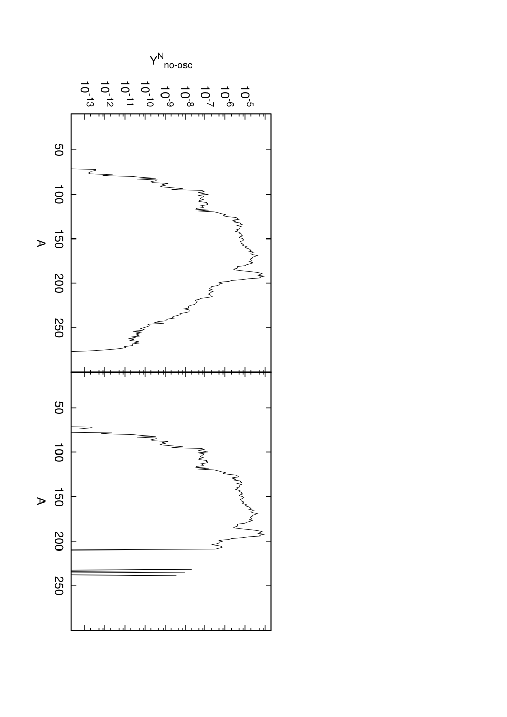
We have solved the full system of equations until neutron freeze-out occurs, that is when the value of the abundance of neutrons relative to protons reaches unity, and for the high-entropy wind scenario [47]. To characterize the wind, we have chosen the initial temperature , the density profile where is the initial density and [48, 46, 59, 60]. The initial electron fraction considered is , the wind speed of expansion and the initial wind radius [30, 61]. Figure 1 shows the results for the calculated abundances, without including neutrino oscillations, and for different parametrizations of the fission channel. The abundances for nuclei around for the no-fission case are smaller than those obtained by allowing fission. The results corresponding to the full fission case agree with the ones reported in Ref. [62], obtained by using SMOKER [54] and ALBA [63].

In Figure 2 we show the results for nuclear abundances calculated without including neutrino oscillations [50, 51], for two different values of the time needed to reach stability after the r-process, . An arbitrary large value of the stability time, as the one used in the calculations, implies that the nuclei are allowed to decay, but in spite of this we found nuclear species with masses up to A= (e.g: 232Th ( and ), 235U and 238U ( and , ), etc.
Neutrino oscillations are turned on by replacing in the code the conventional expressions for the decay rate of Eq.(5) by the decay rates in presence of neutrino oscillations, of Eq.(6). Table 1 shows the changes affecting the beta decay rates due to neutrino oscillations and mixing, as expressed by the factor of Eq.(17). For all cases shown in the table, we have used the values , and for the active sector the parameters 0.09 and . It is seen that the factor depends strongly on the value of the mixing angle between active and sterile neutrino species. Naturally, realistic values of the ratio are limited by the known estimates of beta decay transitions and their renormalization factors in nuclei. What we are showing in this table is the dependence of with the mixing angle. The deviations from the values obtained with structureless neutrinos are of the order of few percents, for larger values of .
| \toprule | ratio f | |
|---|---|---|
| \colrule | 0.00105 | 1.00000 |
| 0.00113 | 0.99901 | |
| 0.00112 | 0.99606 | |
| 0.00110 | 0.97553 | |
| \botrule |
We have used different oscillation parameters to describe the mixing between active neutrinos and a sterile neutrino, and took two values of the stability time . The code was used with the initial distribution of mass-fractions corresponding to an entropy of (in units of 100 times the Boltzmann constant) [64], this value is consistent with the late cooling-time of supernovae and with the generation of the neutrino driven wind. The results of the calculations are presented next.
3.1 Results including neutron-capture and beta-decay in the calculation of nuclear abundances.
Figure 3 shows the rate between the abundances calculated with and without including neutrino oscillations, for two different values of the stability time . In the caption to the figure we indicate the values of , , and . The other parameters for neutrino-oscillations are taken from Ref.[30, 44].

It is seen from the results displayed in Figure 3 that, when active neutrino-oscillations are included in the treatment, both the beta-decay rate and abundance of nuclei remain invariant with respect to the case without oscillations (top panel of Figure 3). Instead, for the case in which the oscillation with a sterile neutrino is turned-on the abundances increase for nuclear masses up to A=100 and decrease for masses larger than A180 respect to the standard case (bottom panel). For larger values of the mixing angle this effect becomes larger. The abundances that are most affected are those corresponding to the nuclei in the region with values of A between 70 and 125, in particular , , , , , even for small mixing angles .
Since the time to stability was fixed to zero, meaning that the nuclei reach stability once they are produced, a larger abundance of heavy elements with A200 is found (left inset of Figure 3). The effect produced by active-sterile neutrino-mixing is smaller for larger values of the time needed to reach stability after the r-process, as one can observed from the curves shown in the right-hand inset of Figure 3.
3.2 Results taken a complete set of reaction in the equations.
We study the problem considering all the reactions which determine the nuclear abundances, that is -decay [49], -capture, beta-decay [50, 51], beta-decay of delayed neutrons [51], neutron-emission, neutron-capture [52], photo-dissociation [52] and fission.
In Figure 4 we show the ratio between the nuclear abundances with and without including neutrino-mixing, and for . Again, the oscillations between active flavors do not generate changes with respect to the standard case, that is without neutrino oscillations. The inclusion of active-sterile neutrino mixing increases the abundances for A75 with respect to the standard case. This effect is different than the one obtained in the previous section. A peak indicating an overproduction around appears in all cases studied, the peak intensifies when the mixing angle is larger. The parameters adopted for the mixing with the sterile neutrino sector are given in the caption to the figure.

The results of the calculation of the abundances of heavy-mass nuclei, excluding fission, are presented in Figure 5. Also in this case the inclusion of active-sterile neutrino-mixing has an effect upon the predicted abundances.

4 Conclusions
In this work we have calculated beta-decay-rates in presence of neutrino oscillations and used them to calculate differential decay-rates entering in rapid neutron-capture-processes leading to the production of heavy mass nuclei in core-collapse SN.
We found that the mixing between active neutrino flavors does not affect the decay rate or the abundances produced by the rapid process. In contrast, we have found that the beta-decay rate decreases when the neutrino-mixing with a sterile specie is taken into account. The impact on the calculated neutron-decay-rate depends strongly on the mixing angle , and weakly on the mass-square difference . Accordingly, we have renormalized the decay rates of heavy nuclei and used them to calculate nuclear abundances in the context of the r-process.
For the case in which only the main reactions are considered the change in beta decay rates, due to active-sterile neutrino mixing, generates changes in the abundances. In particular, for A 150, the nuclear abundances increase while for A 150 they decrease, both cases with respect to the results obtained in standard calculations which omit neutrino mixing. The changes in the predicted nuclear abundances are larger for larger values of the mixing angle .
The abundances of the elements , , , and , are the most sensitive against the inclusion of active-sterile mixing, even for small mixing angles .
Also, we have studied the behavior of abundances for different values of the time needed to reach stability. If we do not allow the nuclei to decay, that is by taking , the code predicts a large abundance of heavy-mass nuclei with A 200. Letting the nuclei decay towards stability, that is for a finite value of , the abundance of nuclei with A200 concentrates around .
Finally, we have performed the analysis including all the reactions in the equations solved by the code. It is found that the predicted abundances change when the active-sterile neutrino-mixing is included in the calculations.
We may conclude by saying that the inclusion of massive active and sterile neutrinos and their mixing seems to be relevant to estimate the viability of the r-process and thus to predict the final abundances of nuclear masses.
Acknowledgment
This work was supported by a grant (PIP-616) of the National Research Council of Argentina (CONICET), and by a research-grant (PICT No. 140492 ) of the National Agency for the Promotion of Science and Technology (ANPCYT) of Argentina. O. C. and M. E. M. are members of the Scientific Research Career of the CONICET, M. M. S. is a Ph.D fellow of the CONICET.
References
- [1] M.-R. Wu, G. Martinez-Pinedo, and Y.-Z. Qian, in 13th International Symposium on Origin of Matter and Evolution of the Galaxies (OMEG2015) Beijing, China, June 24-27, 2015 (2015), 1512.030630.
- [2] Y. Z. Qian, G. M. Fuller, G. J. Mathews, R. W. Mayle, J. R. Wilson, and S. E. Woosley, Phys. Rev. Lett. 71, 1965 (1993).
- [3] S. E. Woosley, J. R. Wilson, G. J. Mathews, R. D. Hoffman, and B. S. Meyer, ApJ 433, 229 (1994).
- [4] O. Civitarese, M. E. Mosquera, and M. M. Sáez, International Journal of Modern Physics E 23, 1450080 (2014).
- [5] M. E. Mosquera, and O. Civitarese, Phys. Rev. C 84, 065803 (2011).
- [6] M. E. Mosquera, and O. Civitarese, Journal of Cosmology and Astro-Particle Physics 2015, 038 (2015).
- [7] M. M. Saez, O. Civitarese and M. E. Mosquera, Int. J. Mod. Phys. D 27, no. 12, 1850116 (2018).
- [8] A. Aguilar-Arevalo et al. (LSND), Phys. Rev. D 64, 112007 (2001).
- [9] Y. Fukuda et al. (Super-Kamiokande), Phys. Rev. Lett. 81, 1562 (1998).
- [10] A. W. P. Poon et al. (SNO), AIP Conf. Proc. 610, 218 (2002).
- [11] A. A. Aguilar-Arevalo et al. (MiniBoNE), Phys. Rev. Lett. 98, 231801 (2007).
- [12] A. A. Aguilar-Arevalo et al. (MiniBoNE), Phys. Rev. Lett. 110, 161801 (2013).
- [13] C. Palomares (Double Chooz), PoS EPS-HEP2009, 275 (2009).
- [14] J. N. Abdurashitov et al. (SAGE), Phys. Rev. C 80, 015807 (2009).
- [15] J. A. Detwiler (KamLAND), eConf C0307282, TW04 (2003).
- [16] C. Arpesella et al. (Borexino), Phys. Rev. Lett. 101, 091302 (2008).
- [17] K. Eitel, New Journal of Physics 2, 1 (2000).
- [18] C. Athanassopoulos et al., Phys. Rev. Lett. 75, 2650 (1995).
- [19] C. Athanassopoulos et al. (LSND), Phys. Rev. Lett. 77, 3082 (1996).
- [20] A. A. Aguilar-Arevalo et al. (MiniBooNE), Phys. Rev. Lett. 121, no. 22, 221801 (2018).
- [21] C. Giunti and M. Laveder, Phys. Rev. D 84, 073008 (2011).
- [22] A. Himmel, Physics Procedia 61, 612 (2015), 13th International Conference on Topics in Astroparticle and Underground Physics, TAUP 2013.
- [23] A. Boyarsky, O. Ruchayskiy and M. Shaposhnikov, Ann. Rev. Nucl. Part. Sci. 59, 191 (2009).
- [24] R. N. Mohapatra and P. B. Pal, Massive Neutrinos in Physics and Astrophysics, Lecture Notes in Physics Series (World Scientific, 2004). ISBN 9789812380715.
- [25] G. G. Raffelt, and D. Seckel, Phys. Rev. Lett. 60, 1793 (1988).
- [26] A. Molinari, L. Riccati and W. M. Alberico, From Nuclei and Their Constituents to Stars International School of Physics Enrico Fermi (IOS Press, 2003), ISBN 9781614990093.
- [27] K. G. Balasi, K. Langanke, and G. Martinez-Pinedo, Prog. Part. Nucl. Phys. 85, 33 (2015).
- [28] J. Fetter, G. C. McLaughlin, A. B. Balantekin and G. M. Fuller, Astropart. Phys. 18, 433 (2003).
- [29] A. Balantekin and H. Yuksel, New J. Phys. 7, 51 (2005).
- [30] I. Tamborra, G. G. Raffelt, and D. V Semikoz, JCAP 1, 13 (2012).
- [31] H.-T. Janka, Ann. Rev. Nucl. Part. Sci. 62, 407 (2012).
- [32] S. Pastor, G. G. Raffelt, and D. V. Semikoz, Phys. Rev. D 65, 053011 (2002).
- [33] Y.-Z. Qian, Prog. Part. Nucl. Phys. 50, 153 (2003).
- [34] E. Anders and N. Grevesse, Geochim. Cosmochim. Acta 53, 197 (1989).
- [35] H. Duan, A. Friedland, G. C. McLaughlin and R. Surman, J. Phys. G 38, 035201 (2011).
- [36] D. Kasen et al., Nature 551, 7678 (2017)
- [37] J. J. Cowan, C. Sneden, J. E. Lawler, A. Aprahamian, M. Wiescher, K. Langanke, G. Martínez-Pinedo and F. K. Thielemann, arXiv:1901.01410 [astro-ph.HE].
- [38] S. Curtis, K. Ebinger, C. Fröhlich, M. Hempel, A. Perego, M. Liebendörfer and F. K. Thielemann, Astrophys. J. 870, no. 1, 2 (2019).
- [39] D. D. Clayton, Principles of stellar evolution and nucleosynthesis: with a new preface (University of Chicago Press, 1968), ISBN 9780226109527.
- [40] R. E. Marshak, Riaduzzin and C. P. Ryan, Theory of weak interactions in particle physics (Wiley-Interscience; New York, 1969).
- [41] R.J. Blin-Stoyle, Fundamental Interactions and the Nucleus [By] R.J. Blin-Stoyle (North-Holland Publishing Company; New York: American Elsevier Publishing Company, 1973).
- [42] W. M. Yao et al., Journal of Physics G 33, 1 (2006).
- [43] A. N. Ivanov, R. Reda and P. Kienle, (2008), 0801.2121.
- [44] R. N. Cahn D. A. Dwyer, S. J. Freedman, W. C. Haxton, R. W. Kadel, Yu. G. Kolomensky, K. B. Luk, P. McDonald, G. D. Orebi Gann, and A. W. P. Poon, in Proceedings, 2013 Community Summer Study on the Future of U.S. Particle Physics: Snowmass on the Mississippi (CSS2013): Minneapolis, MN, USA, July 29-August 6, 2013 (2013), 1307.5487.
- [45] A. Meregaglia. (The Double Chooz Collaboration), Nuovo Cimento Geophysics Space Physics C, 38, 123 (2016).
- [46] C. Charignon, M. Kostka, N. Koning, P. Jaikumar and R. Ouyed, Astron. Astrophys. 531, A79 (2011).
- [47] M. Kostka, N. Koning, Z. Shand, R. Ouyed and P. Jaikumar, Astron. Astrophys. 568, A97 (2014).
- [48] M. Kostka, N. Koning, Z. Shand, R. Ouyed and P. Jaikumar (2014), arXiv:1402.3824 [astro-ph.IM].
- [49] K. R. Lang, Astrophysical Formulae. A Compendium for the Physicist and Astrophysicist. (Springer-Verlag Berlin Heidelberg New York. Also Springer Study Edition, 1980).
- [50] P. Möller, J. R. Nix, W. D. Myers, and W. J. Swiatecki, Atomic Data and Nuclear Data Tables 59, 185 (1995).
- [51] P. Möller, B. Pfeiffer, and K. L. Kratz, Phys. Rev. C 67, 055802 (2003).
- [52] S. Goriely, S. Hilaire and A. J. Koning, Astron. Astrophys. 487, 767 (2008).
- [53] T. Kodama and K. Takahashi, Nuclear Physics A 239, 489 (1975).
- [54] I. V. Panov, E. Kolbe, B. Pfeiffer, T. Rauscher, K. L. Kratz, and F. K. Thielemann, Nucl. Phys. A 747, 633 (2005).
- [55] S. Goriely, S. Hilaire, A. J. Koning, M. Sin, and R. Capote, Phys. Rev. C 79, 024612 (2009).
- [56] J. Benlliure, K. H. Schmidt, A. Grewe, M. de Jong and S. Zhdanov, Nucl. Phys. A 628, 458 (1998).
- [57] B. Jurado and K. H. Schmidt, J. Phys. G 42, no. 5, 055101 (2015).
- [58] M. B. Chadwick et al., Nuclear Data Sheets 107, 2931 (2006).
- [59] B. S. Meyer, G. J. Mathews, W. M. Howard, S. E.Woosley and R. D. Hoffman, ApJ 399, 656 (1992).
- [60] B. S. Meyer and J. S. Brown, The Astrophysical Journal Supplement Series 112, 199 (1997).
- [61] M. R. Wu, T. Fischer, L. Huther, G. Martínez-Pinedo and Y. Z. Qian, Phys. Rev. D 89, no. 6, 061303 (2014).
- [62] I. Petermann, K. Langanke, G. Martinez-Pinedo, P. v. Neumann-Cosel, F. Nowacki and A. Richter, Phys. Rev. C 81, 014308 (2010).
- [63] J. J. Gaimard and K. H. Schmidt, Nucl. Phys. A 531, 709 (1991).
- [64] K. Farouqi, K. L. Kratz, B. Pfeiffer, T. Rauscher, F. K. Thielemann, and J. W. Truran, ApJ 712, 1359 (2010).