跳到论文正文
W Papers独立论文阅读器 arXiv:2006.07904 论文正文 计算阅读时间 · 0%
引用这篇论文根据当前论文元数据生成,正式投稿前建议核对。


License: arXiv.org perpetual non-exclusive license
arXiv:2006.07904v2 [stat.ML] 30 Jul 2020

An Analysis of Constant Step Size SGD in the Non-convex Regime: Asymptotic Normality and Bias

Lu Yu     Krishnakumar Balasubramanian     Stanislav Volgushev     Murat A. Erdogdu Thanks:  Department of Statistical Sciences at the University of Toronto, and Vector Institute˜˜luyu@utstat.toronto.edu Thanks:  Department of Statistics, University of California, Davis˜˜kbala@ucdavis.edu Thanks:  Department of Statistical Sciences at the University of Toronto˜˜stanislav.volgushev@utoronto.ca Thanks:  Department of Computer Science and Department of Statistical Sciences at the University of Toronto, and Vector Institute˜˜erdogdu@cs.toronto.edu
Abstract

Structured non-convex learning problems, for which critical points have favorable statistical properties, arise frequently in statistical machine learning. Algorithmic convergence and statistical estimation rates are well-understood for such problems. However, quantifying the uncertainty associated with the underlying training algorithm is not well-studied in the non-convex setting. In order to address this short-coming, in this work, we establish an asymptotic normality result for the constant step size stochastic gradient descent (SGD) algorithm—a widely used algorithm in practice. Specifically, based on the relationship between SGD and Markov Chains [DDB19], we show that the average of SGD iterates is asymptotically normally distributed around the expected value of their unique invariant distribution, as long as the non-convex and non-smooth objective function satisfies a dissipativity property. We also characterize the bias between this expected value and the critical points of the objective function under various local regularity conditions. Together, the above two results could be leveraged to construct confidence intervals for non-convex problems that are trained using the SGD algorithm.

1 Introduction

Non-convex learning problems are prevalent in modern statistical machine learning applications such as matrix and tensor completion [GHJY15, GLM16, XYZ19, CLC19, CLPC19], deep neural networks [GBC16, JK17, MIG+19], and robust empirical risk minimization [Loh17, LLM18, MBM18]. Developing theoretically principled approaches for tackling such non-convex problems depends critically on the interplay between two aspects. From a computational perspective, variants of stochastic gradient descent (SGD) converge to first-order critical points [GL13, FLLZ18] or local minimizers [NP06, GHJY15, JGN+17, TSJ+18] of the objective function. From a statistical perspective, oftentimes these critical points or local minimizers have nice statistical properties [Kaw16, GLM16, Loh17, MMMO17, EvdG18, CLC19]; see also [FD82] for a counterexample. For the purpose of uncertainty quantification in such non-convex learning paradigms, studying the fluctuations of iterative algorithms used for training becomes extremely important. In this work, we focus on the widely used constant step size SGD, and develop results for quantifying the uncertainty associated with this algorithm for a class of non-convex problems.

Specifically, we consider minimizing a non-smooth and non-convex objective function f:ℝd→ℝf\!:\mathbb{R}^{d}\!\to\mathbb{R},

minθ∈ℝd​f​(θ).\displaystyle\underset{{\theta\in\mathbb{R}^{d}}}{\min}~f(\theta). (1.1)

The iterations of SGD with a constant step size η>0\eta>0, initialized at θ0(η)≡θ0∈ℝd\theta^{(\eta)}_{0}\equiv\theta_{0}\in\mathbb{R}^{d}, are given by

θk+1(η)=θk(η)−η⁡(∇f​(θk(η))+ξk+1​(θk(η))),k≥0,\displaystyle\theta^{(\eta)}_{k+1}=\theta^{(\eta)}_{k}-\eta\big(\nabla f(\theta^{(\eta)}_{k})+\xi_{k+1}(\theta^{(\eta)}_{k})\big),~~~k\geq 0\,, (1.2)

where {ξk}k≥1\{\xi_{k}\}_{k\geq 1} is a sequence of random functions from ℝd\mathbb{R}^{d} to ℝd\mathbb{R}^{d} corresponding to the stochasticity in the gradient estimate. Several problems in machine learning and statistics are naturally formulated as the optimization problem is (1.1), where the function f⁡(θ)f(\theta) is given by

f⁡(θ)≔𝔼Z​[F⁡(θ,Z)]=∫F⁡(θ,Z)​𝑑P​(Z),\displaystyle f(\theta)\coloneqq\mathbb{E}_{Z}[F(\theta,Z)]=\int F(\theta,Z)\,dP(Z), (1.3)

where the function F⁡(θ,Z)F(\theta,Z) is typically the loss function composed with functions from hypothesis class parametrized by θ∈ℝd\theta\in\mathbb{R}^{d}, and depends on the random variable Z∈ℝpZ\in\mathbb{R}^{p}. The distribution P⁡(Z)P(Z) is typically unknown. Then the iterations of online SGD with a constant step size η>0\eta>0, and batch-size bkb_{k}, initialized at θ0(η)≡θ0∈ℝd\theta^{(\eta)}_{0}\equiv\theta_{0}\in\mathbb{R}^{d}, are given by

θk+1(η)=θk(η)−ηbk​∑j=1bk∇F​(θk(η),Zj),k≥0,\displaystyle\theta^{(\eta)}_{k+1}=\theta^{(\eta)}_{k}-\frac{\eta}{b_{k}}\sum_{j=1}^{b_{k}}\nabla F(\theta^{(\eta)}_{k},Z_{j}),~~~k\geq 0\,, (1.4)

where independent samples Zj∼P⁡(Z)Z_{j}\sim P(Z), is used to estimate the true gradient in each iteration kk. Furthermore, the samples ZjZ_{j} used across all iterates kk are also independent. Typically, we also have ∇F​(θ,Z)\nabla F(\theta,Z) to be unbiased estimates of the true gradient ∇f​(θ)\nabla f(\theta), for all θ∈ℝd\theta\in\mathbb{R}^{d}. The above iterates are indeed a special case of the iterates in (1.2), with the noise sequence {ξk​(θk(η))}k≥1\{\xi_{k}(\theta^{(\eta)}_{k})\}_{k\geq 1} given by

ξk​(θk(η)):=1bk​∑j=1bk[∇F​(θk(η),Zj)−∇f​(θk(η))].\displaystyle\xi_{k}(\theta^{(\eta)}_{k}):=\frac{1}{b_{k}}\sum_{j=1}^{b_{k}}\left[\nabla F(\theta^{(\eta)}_{k},Z_{j})-\nabla f(\theta^{(\eta)}_{k})\right]. (1.5)

Although proposed in the 1950s by [RM51], SGD has been the algorithm of choice for training statistical models due to its simplicity, and superior performance in large-scale settings [FP99, DDB19, WRS+17, BH18]. However, the fluctuations of this algorithm is well-understood only when the objective function ff is strongly convex and smooth, and the step size η\eta satisfies a specific decreasing schedule so that the iterates asymptotically converge to the unique minimizer [PJ92, DR18, ABE19]. On the other hand, it is well-known that the SGD iterates in (1.2) can be viewed as a Markov chain which allows them to converge to a random vector rather than a single critical point [DDB19]. Building on this analogy between SGD and Markov chains, the aforementioned shortcomings can be alleviated by simply relaxing the global smoothness as well as the strong convexity assumptions to the tails of the objective function ff, which allows for non-convex structure around the region of interest. Similar kinds of tail relaxations have been successfully employed in the diffusion theory when the target potential is non-convex [RRT17, CCAY+18, EMS18], but they are not studied in the context of non-convex optimization with the SGD algorithm. In this work, we study the fluctuations and the bias of the averaged SGD iterates in (1.2), around the first-order critical points of the minimization problem (1.1). Our contributions can be summarized as follows.

  • •

    For a non-convex and non-smooth objective function ff with tails growing at least quadratically, we establish the uniqueness of the stationary distribution of the constant step size SGD iterates in Proposition 2.1, and the asymptotic normality of Polyak-Ruppert averaging in Theorem 2.1. To the best of our knowledge, these are the first uniqueness and normality results for the SGD algorithm when the objective function is non-convex (even not strongly convex) and non-smooth.

  • •

    We further show in Proposition 3.1 that, under the assumptions leading to the CLT, the asymptotic bias between the expectation of the Lipschitz test function ϕ\phi under the stationary distribution of the SGD iterates and the value of ϕ\phi at any first-order critical point is bounded by a constant depending on the tail growth properties of ff.

  • •

    Finally, we show in Theorems 3.1 and 3.2 that with additional local smoothness assumptions on the function ff that allow non-convexity, we can establish a control over the bias in terms of step size. We further characterize the bias when the objective is (not strongly) convex in Theorem 3.3, providing a thorough bias analysis for the constant step size SGD under various settings that are frequently encountered in statistics.

Our results provide algorithm-dependent guarantees for uncertainty quantification, and they could be potentially leveraged to obtain confidence intervals for non-convex and non-smooth learning problems. This is contrary to the majority of the existing results in statistics, which only establish normality results for the true stationary point of the non-convex objective function; see for example [Loh17, QCLP19]. While being useful, such results completely ignore the computational hardships associated with non-convex optimization; hence, their practical implications are limited. On the other hand, in the optimization and learning theory literature, a majority of the existing results establish the rate of convergence of an algorithm to a critical point, and do not quantify the fluctuations associated with that algorithm. Our work bridges these separate lines of thought by providing asymptotic normality results directly for the SGD algorithm used for minimizing non-convex and non-smooth functions.

More Related Works. Establishing asymptotic normality results for the SGD algorithm began with the works of [Chu54, Sac58, Fab68, Rup88, Sha89], with [PJ92] providing a definitive result for strongly convex objectives. In particular, [PJ92] and [Rup88] established that the averaged SGD iterates with an appropriately chosen decreasing step size is asymptotically normal with the variance achieving the Cramer-Rao lower bound for parameter estimation. Recent works, for example [TFBJ18, SZ18, DR18, TA17, FXY18], leverage the asymptotic normality analysis of [PJ92], and compute confidence intervals for SGD. The benefits of constant step size SGD for faster convergence under overparametrization has also be demonstrated in the works of [SR13, NWS14, MBB18, VBS19]. The use of Markov chain theory to study constant step size stochastic approximation algorithms has been considered in several works [Kif88, Ben96, PV98, FP99, AMP00, TV19]. Recently, [DDB19, CT18] investigated the asymptotic variance of constant step size SGD. We emphasize here that most of the above works assume strongly convex and smooth objective functions. Finally, there exists a vast literature on analyzing Markov chain Monte Carlo sampling algorithms based on discretizing diffusions. We refer the interested reader to [DK17, BDMP17, CCAY+18, DM17, Dal17, CCBJ17, BEL18, DCWY18, DRD18, LWME19, SL19, EH20] and the references therein, for details.

Notation. For a,b∈ℝa,b\in\mathbb{R}, denote by a∨ba\vee b and a∧ba\wedge b the maximum and the minimum of aa and bb, respectively. We use ∥⋅∥\|\cdot\| to denote the Euclidean norm in ℝd\mathbb{R}^{d}. We denote the largest eigenvalue of the matrix AA as λmax​(A),\lambda_{\max}(A), and the smallest one as  λmin​(A).\lambda_{\min}(A). Let (Ω,ℱ,ℙ)(\Omega,\mathcal{F},\mathbb{P}) represent a probability space, and denote by ℬ⁡(ℝd)\mathcal{B}(\mathbb{R}^{d}), the Borel σ\sigma-field of ℝd\mathbb{R}^{d}. Let 𝒫k​(ℝd):={ν:∫ℝd‖θ‖k​ν​(𝑑θ)<∞}\mathcal{P}_{k}(\mathbb{R}^{d}):=\{\nu:\int_{\mathbb{R}^{d}}\|\theta\|^{k}\nu(d\theta)<\infty\} denote the set of probability measures with finite kk-th moments. For a probability distribution π\pi and a function gg on 𝒳\mathcal{X}, we define π⁡(g)≔∫𝒳g⁡(x)​𝑑π​(x)\pi(g)\coloneqq\int_{\mathcal{X}}g(x)d\pi(x), and ℒ2(π):={g:𝒳→ℝ:π(g2)<∞}.\mathcal{L}_{2}(\pi):=\{g:\mathcal{X}\to\mathbb{R}:\pi(g^{2})<\infty\}.

2 Central Limit Theorem for The Constant Step Size SGD

In this section, we establish an asymptotic central limit theorem (CLT) for the Polyak-Ruppert averaging of the constant step size SGD iterates given in (1.2) when the objective function is potentially non-convex, non-smooth, and has quadratically growing tails. More specifically, we first prove that there exists a unique stationary distribution πη∈𝒫2​(ℝd)\pi_{\eta}\in\mathcal{P}_{2}(\mathbb{R}^{d}) for the Markov chain defined by the SGD algorithm when the objective function is dissipative (see Assumption 2.2) with gradient exhibiting at most linear growth (see Assumption 2.1). Furthermore, under the same conditions, we prove that a CLT holds for the Polyak-Ruppert averaging, and it is independent of the initialization. In what follows, we list and discuss the main assumptions required to establish a CLT for the SGD iterates, and compare them to those existing in the literature.

Assumption 2.1 (Linear growth).

The gradient of the objective function ff has at most linear growth. That is, for some L≥0L\geq 0, we have

‖∇f​(θ)‖≤L⁡(1+‖θ‖) for all θ∈ℝd.\displaystyle\|\nabla f(\theta)\|\leq L\big(1+\|\theta\|\big)\ \ \text{ for all }\ \ \theta\in\mathbb{R}^{d}. (2.1)

Majority of the results on SGD focus on smooth functions with gradients satisfying ‖∇f​(θ)−∇f​(θ′)‖≤‖θ−θ′‖\|\nabla f(\theta)-\nabla f(\theta^{\prime})\|\leq\|\theta-\theta^{\prime}\| for all θ,θ′∈ℝd\theta,\theta^{\prime}\in\mathbb{R}^{d}; see e.g. [PJ92, DDB19]. The above condition allows for non-smooth objectives, and is a significant relaxation of the standard Lipschitz gradient condition.

Assumption 2.2 (Dissipativity).

The objective function ff is (α,β)(\alpha,\beta)-dissipative. That is, there exists positive constants α,β\alpha,\beta such that

⟨θ,∇f​(θ)⟩≥α​‖θ‖2−β for allθ∈ℝd.\displaystyle\langle\theta,\,\nabla f(\theta)\rangle\geq\alpha\,\|\theta\|^{2}-\beta\ \ \text{ for all}\ \ \theta\in\mathbb{R}^{d}. (2.2)

The dissipativity assumption has its origins in the analysis of dynamical systems, and is used widely in the analysis of optimization and learning algorithms [MSH02, RRT17, EMS18, XCZG18]. It could be viewed as a relaxation of strong convexity since it restricts the quadratic growth assumption to the tails of the function ff, enforcing no local growth around the first-order critical points. A canonical example for this condition is the sum of a quadratic and any non-convex function with bounded gradient. For example, consider the function x→x2+10​sin⁡(x)x\to x^{2}+10\sin(x) which is clearly non-convex and (1,25)(1,25)-dissipative. It is worth mentioning that many statistical learning problems such as phase retrieval [TV19] satisfy Assumption 2.2.

Assumption 2.3 (Noise sequence).

Gradient noise sequence {ξk}k≥1\{\xi_{k}\}_{k\geq 1} is a collection of i.i.d. random fields satisfying

𝔼⁡[ξ1​(θ)]=0​and ​𝔼1/2​[‖ξ1​(θ)‖2]≤Lξ​(1+‖θ‖),\displaystyle\mathbb{E}[\xi_{1}(\theta)]=0\,\ \text{and }\ \mathbb{E}^{1/2}[\|\xi_{1}(\theta)\|^{2}]\leq L_{\xi}(1+\|\theta\|)\,, (2.3)

for any θ∈ℝd\theta\in\mathbb{R}^{d} and a positive constant LξL_{\xi}. Moreover, for each θ∈ℝd\theta\in\mathbb{R}^{d} the distribution of the random variable ξ1​(θ)\xi_{1}(\theta) can be decomposed as μ1,θ+μ2,θ\mu_{1,\theta}+\mu_{2,\theta} where μ1,θ\mu_{1,\theta} has a density, say pθp_{\theta}, with respect to Lebesgue measure which satisfies infθ∈Cpθ​(t)>0\inf_{\theta\in C}p_{\theta}(t)>0 for any bounded set CC and any t∈ℝpt\in\mathbb{R}^{p}.

Assumption 2.3 as formulated above is stronger than what is used in the proofs. It can easily be seen that the lower bound on the density pθp_{\theta} is only required to hold for a specific set whose form depends on η\eta and various constants from Assumptions 2.1–2.3. The form of this set is complicated, and an exact expression is given in the Appendix – see equation (A.4). We also emphasize that Assumption 2.3 also does not specify any explicit parametric form for the distribution of the noise sequence contrary to recent works in non-convex settings where dissipitavity condition has been heavily utilized [RRT17, XCZG18, EMS18].

We now establish the existence and uniqueness of the stationary distribution of the SGD iterates (1.2).

Proposition 2.1 (Ergodicity of SGD).

Let the Assumptions 2.1-2.3 hold. For a step size satisfying

η<α−(α2−(3​L2+Lξ))∨03​L2+Lξ,\eta<\frac{\alpha-\sqrt{\bigl(\alpha^{2}-{(3L^{2}+L_{\xi})}\bigr)\vee 0}}{{3L^{2}+L_{\xi}}}\,,

the following statements hold for the SGD (1.2).

  1. (a)

    SGD iterates admit a unique stationary distribution πη∈𝒫2​(ℝd)\pi_{\eta}\in\mathcal{P}_{2}(\mathbb{R}^{d}), depending on the choice of step size η\eta.

  2. (b)

    For a test function ϕ:ℝd→ℝ\phi:\mathbb{R}^{d}\to\mathbb{R} satisfying |ϕ⁡(θ)|≤Lϕ​(1+‖θ‖)|\phi(\theta)|\leq L_{\phi}(1+\|\theta\|) ∀θ∈ℝd\forall\theta\in\mathbb{R}^{d} and some Lϕ>0L_{\phi}>0, and for any initialization θ0(η)=θ0∈ℝd\theta_{0}^{(\eta)}=\theta_{0}\in\mathbb{R}^{d} of the SGD algorithm, there exists ρ∈(0,1)\rho\in(0,1) and κ\kappa (both depending on η\eta) such that we have

    |𝔼⁡[ϕ⁡(θk(η))]−πη​(ϕ)|≤κ​ρk​(1+‖θ0‖2),\big|\mathbb{E}\big[\phi\big(\theta_{k}^{(\eta)}\big)\big]-\pi_{\eta}(\phi)\big|\leq\kappa\,\rho^{k}(1+\|\theta_{0}\|^{2}),

    where πη​(ϕ)≔∫ϕ⁡(x)​d​πη​(x)\pi_{\eta}(\phi)\coloneqq\int\phi(x)d\pi_{\eta}(x).

The uniqueness of the stationary distribution of the constant step size SGD has been established in [DDB19] for strongly convex and smooth objectives. In Proposition 2.1, we relax both of these assumptions allowing for non-convex and non-smooth objectives. Our proof relies on VV-uniform ergodicity [MT12], which is fundamentally different from the ergodicity analysis in [DDB19]. Under the dissipativity condition (quadratic growth of ff), geometric ergodicity in Proposition 2.1 is not surprising; yet, it is worth highlighting that the function ff as well as the noise sequence require significantly less structure than what was assumed in the literature. The above step size assumption is almost standard and it is required to obtain a uniform bound on the moments of SGD iterates. We highlight that similar to the gradient descent algorithm, the step size depends on a quantity that serves as a surrogate condition number in our setting, namely, L/αL/\alpha. For the purposes of establishing a CLT, it is sufficient to consider moments of order 4 (in fact any order larger than 2 suffices), but it is also worth noting that any order moments of SGD can be controlled under Assumption 2.2 as long as the noise has the same order finite moment.

Next, we state our first principal contribution, a central limit theorem for the averaged SGD iterates starting from any initial distribution for a non-convex objective. For a test function ϕ:ℝd→ℝ\phi:\mathbb{R}^{d}\to\mathbb{R}, we denote the centered partial sums of ϕ\phi evaluated at the SGD iterates with Sn​(ϕ)S_{n}(\phi), i.e., we define

Sn​(ϕ)≔∑k=0n−1[ϕ⁡(θk(η))−πη​(ϕ)] where πη​(ϕ)≔∫ϕ⁡(x)​d​πη​(x).\displaystyle S_{n}(\phi)\coloneqq\sum_{k=0}^{n-1}\Big[\phi\big(\theta^{(\eta)}_{k}\big)-\pi_{\eta}(\phi)\Big]\ \ \text{ where }\ \ \pi_{\eta}(\phi)\coloneqq\int\phi(x)d\pi_{\eta}(x). (2.4)
Theorem 2.1 (CLT).

Let the Assumptions 2.1-2.3 hold. For a step size η\eta and a test function ϕ\phi satisfying the conditions in Proposition 2.1, we define σπη2​(ϕ)≔limn→∞1n​𝔼πη​[Sn2​(ϕ)]\sigma^{2}_{\pi_{\eta}}(\phi)\coloneqq\lim_{n\to\infty}\frac{1}{n}\mathbb{E}_{\pi_{\eta}}\bigl[S_{n}^{2}(\phi)\bigr]. Then,

n−1/2Sn(ϕ)⟶d𝒩(0,σπη2(ϕ)).\displaystyle n^{-1/2}S_{n}(\phi)\overset{\text{d}}{\longrightarrow}\mathcal{N}\big(0,\sigma^{2}_{\pi_{\eta}}(\phi)\big)\,. (2.5)

The above result characterizes the fluctuations of a test function ϕ\phi averaged across SGD iterates, even when the objective function is both non-convex and non-smooth. The asymptotic variance in the above CLT can be equivalently stated in another compact form. If we define the centered test function as h⁡(θ)=ϕ⁡(θ)−πη​(ϕ)h(\theta)=\phi(\theta)-\pi_{\eta}(\phi), the asymptotic variance can be written as

σπη2​(ϕ)=2​πη​(h​h^)−πη​(h2) where h^=∑k=0∞𝔼⁡[h⁡(θk(η))].\displaystyle\sigma^{2}_{\pi_{\eta}}(\phi)=2\pi_{\eta}(h\hat{h})-\pi_{\eta}(h^{2})\ \ \text{ where }\ \ \hat{h}=\sum_{k=0}^{\infty}\mathbb{E}\Big[h\big(\theta_{k}^{(\eta)}\big)\Big]. (2.6)

Indeed, this is the variance we compute at the end of our proof in Section A. However, the expression in Theorem 2.1 is obtained by simply applying [DMPS18, Thm 21.2.6]. For the case of strongly convex functions with decreasing step size schedule, it is well-known from the works of [PJ92, Rup88] that the limiting variance of the averaged SGD iterates achieves the Cramer-Rao lower bound for parameter estimation; see also [MB11, ABE19] for non-asymptotic rates in various metrics. The question of providing lower bounds for the limiting variance of the critical points in the non-convex setting is extremely subtle, and is often handled on a case-by-case basis. We refer the interested reader to [Gey94, Sha00, Loh17].

There are several important implications of the above CLT result for constructing confidence intervals in practice. First note that, following the standard construction in inference, one can write the distribution of the sample mean approximately as n−1​Sn​(ϕ)≈𝒩⁡(0,n−1​σπη2​(ϕ))n^{-1}S_{n}(\phi)\approx\mathcal{N}\bigl(0,n^{-1}\sigma^{2}_{\pi_{\eta}}(\phi)\bigr). Here, one needs to estimate the population quantity, the asymptotic variance σπη2​(ϕ)\sigma^{2}_{\pi_{\eta}}(\phi), for the purpose of obtaining confidence intervals. In Section 5, we discuss three strategies for estimating this quantity, which could be eventually used for inference in practice. A theoretical analysis of the proposed approaches in Section 5 is beyond the scope of this work.

3 Bias of the Constant Step Size SGD

In this section, we present a thorough analysis of the bias of constant step size SGD algorithm. We first show in Section 3.1 that, in the non-convex and non-smooth case for which we established the CLT, the SGD algorithm converges to a ball that contains all the first-order critical points exponentially fast; nevertheless, the bias is not controllable with the step size. Motivated by this, we provide three types of bias analyses in Section 3.2 under different local growth assumptions on the objective ff, characterizing the bias behavior in various non-convex and convex settings. For this, we strength the assumption of the noise sequence as follows.

Assumption 3.1 (Noise sequence).

Gradient noise sequence {ξk}k≥1\{\xi_{k}\}_{k\geq 1} satisfies Assumption 2.3, and it holds for any θ∈ℝd\theta\in\mathbb{R}^{d} that

𝔼⁡[‖ξ1​(θ)‖4]≤Lξ​(1+‖θ‖4),\displaystyle\mathbb{E}\bigl[\|\xi_{1}(\theta)\|^{4}\bigr]\leq L_{\xi}(1+\|\theta\|^{4})\,, (3.1)

where LξL_{\xi} is the same as in Assumption 2.3.

3.1 Bias without Local Regularity

Bias behavior of an algorithm is intimately related to the local properties of the objective at critical points. Therefore, under the mild assumptions that yield the CLT, one cannot expect a tight control over the bias. However, the tail growth condition is sufficient for a rough characterization, which is still important because even the points that are close to the local minimizers generally have favorable computational [BVB16, MMMO17, CLC19], and statistical properties [Loh17, EvdG18, QCLP19].

If Assumption 2.2 holds for an objective function ff, all first-order critical points of ff must lie inside a ball of radius β/α\sqrt{\beta/\alpha}. Based on this, we show that the SGD iterates (1.2) will move towards this ball exponentially fast, which ultimately establishes a bound on the non-asymptotic bias, and in the limit case yields a bound on the asymptotic bias. The following result formalizes this statement.

Proposition 3.1.

Let Assumptions 2.1,2.2, and 3.1 hold. For θ∗\theta^{*} denoting an arbitrary critical point of the objective function ff, define the constants L¯:=L⁡(1+‖θ∗‖),\bar{L}:=L(1+\|\theta^{*}\|), and

cL,α≔[α−(α2−(3​L2+Lξ))∨0]/[3​L2+Lξ]cL,α†≔[α−(α2−16​L†)∨0]/(64​L†)\displaystyle\begin{split}c_{L,\alpha}&\coloneqq\Bigl[\alpha-\sqrt{\bigl(\alpha^{2}-{(3L^{2}+L_{\xi})}\bigr)\vee 0}\,\Bigr]\big/[{3L^{2}+L_{\xi}}]\\ c_{L,\alpha}^{\dagger}&\coloneqq\Bigl[\alpha-\sqrt{(\alpha^{2}-{16L_{\dagger}})\vee 0}\,\Bigr]\big/{(64{L_{\dagger}})}\end{split} (3.2)

with L†≔L¯2+16​(Lξ3/4​(1+(β/α)3)∨Lξ1/2​(1+(β/α)2)∨Lξ​(1+(β/α)4)).{L_{\dagger}\coloneqq\bar{L}^{2}+16\Bigl(L_{\xi}^{3/4}\bigl(1+(\beta/\alpha)^{3}\bigr)\vee L_{\xi}^{1/2}\bigl(1+(\beta/\alpha)^{2}\bigr)\vee L_{\xi}\bigl(1+(\beta/\alpha)^{4}\bigr)\Bigr).} Then, for SGD iterates initialized at a fixed point θ0∈ℝd\theta_{0}\in\mathbb{R}^{d} and a step size satisfying η<1∧110​L¯∧cL,α∧cL,α†,\eta<1{\wedge\frac{1}{10\bar{L}}}\wedge c_{L,\alpha}\wedge c_{L,\alpha}^{\dagger}\,, we have

𝔼​[‖θk(η)−θ∗‖4]1/2≤ρk​‖θ0−θ∗‖2+D,\displaystyle\mathbb{E}\bigl[\,\|\theta^{(\eta)}_{k}-\theta^{*}\|^{4}\bigr]^{1/2}\leq{\rho}^{\,k}\,\|\theta_{0}-\theta^{*}\|^{2}+D\,, (3.3)

where constants are

D≔\displaystyle D\coloneqq 64α​(L¯4+Lξ​(1+(β/α)4)+512​L¯6+23​Lξ3/2​(1+(β/α)6))1/2\displaystyle\frac{64}{\alpha}\Bigl({\bar{L}^{4}+{L_{\xi}\bigl(1+(\beta/\alpha)^{4}\bigr)+512\bar{L}^{6}+23L_{\xi}^{3/2}\bigl(1+(\beta/\alpha)^{6}\bigr)}}\Bigr)^{1/2} (3.4)
∨8α​(β+(α+2​L/α)2​‖θ∗‖+L​‖θ∗‖+6​L¯2+9​Lξ1/2​(1+(β/α)2)+16),\displaystyle\vee\frac{8}{\alpha}\Bigl(\beta+(\sqrt{\alpha}+2L/\sqrt{\alpha})^{2}\|\theta^{*}\|+L\|\theta^{*}\|+6\bar{L}^{2}+{9L_{\xi}^{1/2}\bigl(1+(\beta/\alpha)^{2}\bigr)}+16\Bigr), (3.5)
ρ≔\displaystyle\rho\coloneqq 1−2​α​η+32​L†​η2∈(0,1).\displaystyle\sqrt{1-2\alpha\eta+32{L_{\dagger}}\eta^{2}}\in(0,1). (3.6)

Consequently, for any test function ϕ\phi that is LϕL_{\phi}-Lipschitz continuous, we have

|πη​(ϕ)−ϕ⁡(θ∗)|≤Lϕ​D.\displaystyle\bigl|\pi_{\eta}(\phi)-\phi(\theta^{*})\bigr|\leq L_{\phi}\sqrt{D}\,. (3.7)

The above theorem establishes that the SGD algorithm initialized far away from any critical point will converge (in the 4-th expectation) to the ball that contains all the first-order critical points exponentially fast. The first term in the upper bound (3.3) depends on the initialization, but decays to zero exponentially fast with the number of iterations, for a fixed step size. The second term in the bound (3.3) is a constant independent of the iteration number as well as the step size, which serves as the squared radius of the ball that contains all the critical points plus an additional offset to account for the randomness in the SGD iterates. In other words, SGD algorithm initialized at any point and with any sufficiently small step size will find this ball of interest exponentially fast.

3.2 Bias with Local Regularity

In this part, we present algorithmically controllable bounds on the bias under local regularity conditions. Section 3.2.1 provides a direct control on 𝔼⁡[‖θk(η)−θ∗‖]\mathbb{E}[\|\theta^{(\eta)}_{k}-\theta^{*}\|] under the assumption that the unique minimizer θ∗\theta^{*} exists. In Sections 3.2.2 and 3.2.3, we characterize the degree of sub-optimality 𝔼⁡[f⁡(θk(η))]−f∗\mathbb{E}[f(\theta^{(\eta)}_{k})]-f^{*} where f∗f^{*} is the global minimum which is not necessarily attained at a unique point.

3.2.1 Localized dissipativity condition

We now introduce the generalized dissipativity condition which, in addition to the tail growth enforced in Assumption 2.2, imposes a local growth around the unique critical point θ∗\theta^{*}.

Assumption 3.2 (Localized dissipativity).

The objective function ff satisfies

⟨∇f​(θ),θ−θ∗⟩≥{α​‖θ−θ∗‖2−β‖θ−θ∗‖≥Rg⁡(‖θ−θ∗‖)‖θ−θ∗‖<R,\displaystyle\langle\nabla f(\theta),\,\theta-\theta^{*}\rangle\geq\begin{cases}\alpha\|\theta-\theta^{*}\|^{2}-\beta&\|\theta-\theta^{*}\|\geq R\\ g\bigl(\|\theta-\theta^{*}\|\bigr)&\|\theta-\theta^{*}\|<R\,,\end{cases} (3.8)

where θ∗∈ℝd\theta^{*}\in\mathbb{R}^{d} is the unique minimizer of ff, R:=δα+βαR:=\frac{\delta}{\alpha}+\sqrt{\frac{\beta}{\alpha}} with δ∈(0,∞)\delta\in(0,\infty), g:[0,∞)→[0,∞)g:[0,\infty)\to[0,\infty) is a convex function with g⁡(0)=0g(0)=0 whose inverse exists.

If g⁡(x)=x2g(x)=x^{2}, the objective function is locally strongly convex. However, the above assumption covers a wide range of objectives with different local growth rates depending on the function gg. Next, we show that the above assumption along with the assumptions leading to the CLT is sufficient to establish an algorithmic control over the bias with a sufficiently small step size.

Theorem 3.1.

Let the Assumptions 2.1, 3.1, and 3.2 hold. Then SGD iterates with step size satisfying η<cL,α\eta<c_{L,\alpha} for cL,αc_{L,\alpha} in (3.2) admit the stationary distribution θ(η)∼πη\theta^{(\eta)}\sim\pi_{\eta} which satisfies

𝔼⁡[‖θ(η)−θ∗‖]≤Cδ​η+g−1​(C​η),\displaystyle\mathbb{E}\bigl[\|\theta^{(\eta)}-\theta^{*}\|\bigr]\leq\frac{C}{\delta}\eta+g^{-1}(C\eta), (3.9)

where

C≔2​(3​L2+3​Lξ1/2​(1+(β/α)2))​(∫‖θ‖2​πη​(𝑑θ)+‖θ∗‖2)+3​L2​‖θ∗‖2+5​L2+2​Lξ1/2​(1+(β/α)2).\displaystyle C\coloneqq{2\Bigl(3L^{2}+3L_{\xi}^{1/2}(1+(\beta/\alpha)^{2})\Bigr)}\Bigl(\int\|\theta\|^{2}\pi_{\eta}(d\theta)+\|\theta^{*}\|^{2}\Bigr)+3L^{2}\|\theta^{*}\|^{2}+5L^{2}+{2L_{\xi}^{1/2}\Bigl(1+(\beta/\alpha)^{2}\Bigr)}\,. (3.10)

Further, for a test function ϕ:ℝd→ℝ\phi:\mathbb{R}^{d}\to\mathbb{R} that is LϕL_{\phi}-Lipschitz, the bias satisfies

|πη​(ϕ)−ϕ⁡(θ∗)|≤Lϕ​(C​η/δ+g−1​(C​η)).\displaystyle\bigl|\pi_{\eta}(\phi)-\phi(\theta^{*})\bigr|\leq L_{\phi}\big({C}\eta/\delta+g^{-1}(C\eta)\big). (3.11)

If the local growth is linear, i.e. g⁡(x)=xg(x)=x, we obtain the bias |πη​(ϕ)−ϕ⁡(θ∗)|≤𝒪⁡(η).|\pi_{\eta}(\phi)-\phi(\theta^{*})|\leq\mathcal{O}(\eta). If local growth is quadratic, i.e. g⁡(x)=x2g(x)=x^{2}, the growth is locally slower than the linear case; thus, we get bias control |πη​(ϕ)−ϕ⁡(θ∗)|≤𝒪⁡(η1/2)|\pi_{\eta}(\phi)-\phi(\theta^{*})|\leq\mathcal{O}(\eta^{1/2}), which is worse in step size dependency, it reduces to the bound derived in [DDB19, Lemma 10].

We highlight that [DCLZ19] prove the following lower bound: liminfk→∞𝔼​[‖θk(η)−θ∗‖2]1/2≥c​η1/2\lim\inf_{k\to\infty}\mathbb{E}[\|\theta^{(\eta)}_{k}-\theta^{*}\|^{2}]^{1/2}\geq c\eta^{1/2} for some c>0c>0 under the assumption of Lipschitz gradients. This is in line with our findings since Lipschits gradients imply g⁡(x)≤x2g(x)\leq x^{2} for small xx.

3.2.2 Generalized Łojasiewicz condition

In this section we work with a generalization of the Łojasiewicz condition.

Assumption 3.3 (Generalized Łojasiewicz condition).

The objective function ff has a critical point θ∗\theta^{*} and it satisfies

‖∇f​(θ)‖2≥{γ⁡{f⁡(θ)−f⁡(θ∗)}‖θ−θ∗‖≥R,g⁡(f⁡(θ)−f⁡(θ∗))‖θ−θ∗‖<R,\displaystyle\|\nabla f(\theta)\|^{2}\geq\begin{cases}\gamma\bigl\{f(\theta)-f(\theta^{*})\bigr\}&\|\theta-\theta^{*}\|\geq R,\\ g\bigl(f(\theta)-f(\theta^{*})\bigr)&\|\theta-\theta^{*}\|<R,\end{cases} (3.12)

where γ\gamma and RR are positive constants, and g:[0,∞)→[0,∞)g:[0,\infty)\to[0,\infty) is a convex function with g⁡(0)=0g(0)=0 whose inverse exists.

In the case g⁡(x)=xκg(x)=x^{\kappa} with κ∈[1,2),\kappa\in[1,2), for example, the above condition is termed as the Łojasiewicz inequality [GLCY16], and for κ=1\kappa=1, it reduces to the well-known Polyak-Łojasiewicz (PL) inequality [KNS16]. Note that this inequality implies that every critical point is a global minimizer; yet, it does not imply the existence of a unique critical point.

The following result establishes an algorithmically controllable bias bound in terms of the step size.

Theorem 3.2.

Let the Assumptions 2.1,2.2, 3.1, and 3.3 hold, and the Hessian satisfies ‖∇2f​(θ)‖≤L~​(1+‖θ‖),\|\nabla^{2}f(\theta)\|\leq\tilde{L}(1+\|\theta\|), ∀θ∈ℝd\forall\theta\in\mathbb{R}^{d}\, and some L~\tilde{L}. Then, the SGD iterates with a step size satisfying η<2L~∧cL,α∧cL,α†∧1\eta<\frac{2}{\tilde{L}}\wedge c_{L,\alpha}\wedge c_{L,\alpha}^{\dagger}\wedge 1 for cL,α,cL,α†c_{L,\alpha},c_{L,\alpha}^{\dagger} in (3.2) have the stationary distribution πη\pi_{\eta},

πη​(f)−f⁡(θ∗)≤g−1​(2​M​η2−L~​η)+2​M​η2−L~​η,\displaystyle\pi_{\eta}(f)-f(\theta^{*})\leq g^{-1}\Bigl(\frac{2M\eta}{2-\tilde{L}\eta}\Bigr)+\frac{2M\eta}{2-\tilde{L}\eta}\,, (3.13)

where

M≔\displaystyle M\coloneqq 12​L~​(L+Lξ1/2+Lξ1/4)2​(1+m+m3/4+∫‖θ‖2​πη​(𝑑θ))​ with\displaystyle 12\tilde{L}\bigl(L+L_{\xi}^{1/2}+L_{\xi}^{1/4}\bigr)^{2}\Bigl(1+m+m^{3/4}+\int\|\theta\|^{2}\pi_{\eta}(d\theta)\Bigr)\ \text{ with } (3.14)
m≔\displaystyle m\coloneqq 87​α​[(β+6​L2+3​Lξ1/2+16)​∫‖θ‖2​πη​(𝑑θ)+16​L4+2​Lξ+128​L6+8​Lξ3/2].\displaystyle\frac{8}{7\alpha}\Bigl[\bigl(\beta+6L^{2}+3L_{\xi}^{1/2}+16\bigr)\int\|\theta\|^{2}\pi_{\eta}(d\theta)+16L^{4}+2L_{\xi}+128L^{6}+8L_{\xi}^{3/2}\Bigr]\,. (3.15)

Additionally, if the test function is given as ϕ=ϕ~∘f\phi=\tilde{\phi}\circ f for a function ϕ~\tilde{\phi} that is Lϕ~L_{\tilde{\phi}}-Lipschitz, it holds that

|πη​(ϕ)−ϕ⁡(θ∗)|≤Lϕ~​{g−1​(2​M​η2−L~​η)+2​M​η2−L~​η}.\displaystyle\bigl|\pi_{\eta}(\phi)-\phi(\theta^{*})\bigr|\leq L_{\tilde{\phi}}\Biggl\{g^{-1}\Bigl(\frac{2M\eta}{2-\tilde{L}\eta}\Bigr)+\frac{2M\eta}{2-\tilde{L}\eta}\Biggr\}. (3.16)

For smooth objectives with Lipschitz gradient, [KNS16] provide a linear rate under the PL-inequality (see also [DYJG17, Lemma 2]), which yields the asymptotic bias |πη​(ϕ)−ϕ⁡(θ∗)|≤𝒪⁡(η).|\pi_{\eta}(\phi)-\phi(\theta^{*})|\leq\mathcal{O}(\eta). The above result recovers their findings as a special case, and provides a considerable generalization.

3.2.3 Convexity

To make the analysis of constant step size SGD complete, we digress from the main theme of this paper and consider the constant step size SGD in the non-strongly convex regime, for which there is no bias characterization known to authors. We show that, under the convexity assumption, one can achieve the same bias control as in the case of PL-inequality.

Theorem 3.3.

Let the Assumptions 2.1,2.2, and 3.1 hold for a convex function ff. Then, the SGD iterates with a step size satisfying η<cL,α\eta<c_{L,\alpha} for cL,αc_{L,\alpha} in (3.2) admit the stationary distribution πη\pi_{\eta}, which satisfies

πη​(f)−f∗≤C​η,\displaystyle\pi_{\eta}(f)-f^{*}\!\leq C\eta\,, (3.17)

where

C≔2​(3​L2+3​Lξ1/2​(1+(β/α)2))​(∫‖θ‖2​πη​(𝑑θ)+‖θ∗‖2)+3​L2​‖θ∗‖2+5​L2+2​Lξ1/2​(1+(β/α)2).\displaystyle C\coloneqq{2\Bigl(3L^{2}+3L_{\xi}^{1/2}(1+(\beta/\alpha)^{2})\Bigr)}\Bigl(\int\|\theta\|^{2}\pi_{\eta}(d\theta)+\|\theta^{*}\|^{2}\Bigr)+3L^{2}\|\theta^{*}\|^{2}+5L^{2}+{2L_{\xi}^{1/2}\Bigl(1+(\beta/\alpha)^{2}\Bigr)}\,. (3.18)

Additionally, if the test function is given as ϕ=ϕ~∘f\phi=\tilde{\phi}\circ f for a function ϕ~\tilde{\phi} that is Lϕ~L_{\tilde{\phi}}-Lipschitz, then,

|πη​(ϕ)−ϕ⁡(θ∗)|≤Lϕ~​C​η.\displaystyle\bigl|\pi_{\eta}(\phi)-\phi(\theta^{*})\bigr|\leq L_{\tilde{\phi}}C\eta. (3.19)

Convexity implies that any critical point θ∗\theta^{*} is a global minimizer, which is similar to the PL-inequality; yet, it does not imply a unique minimizer unlike strong convexity. The resulting step size dependency of the bias is the same as in the case of PL-inequality, which is because both of these conditions assert a similar gradient-based domination criterion on the sub-optimality. That is, we have in the convex case ⟨∇f​(θ),θ−θ∗⟩≥f⁡(θ)−f⁡(θ∗)\langle\nabla f(\theta),\,\theta-\theta^{*}\rangle\geq f(\theta)-f(\theta^{*}), and in the case of PL-inequality γ−1​‖f⁡(θ)‖2≥f⁡(θ)−f⁡(θ∗)\gamma^{-1}\|f(\theta)\|^{2}\geq f(\theta)-f(\theta^{*}).

4 Examples and Numerical Studies

We now demonstrate the asymptotic normality and bias in non-convex optimization with two examples arising in robust statistics for which our assumptions can be verified. We consider the online SGD setting with the update rule (1.4) and also the semi-stochastic setting, where the noise sequence {ξk​(θ)}k≥1\{\xi_{k}(\theta)\}_{k\geq 1} is independent of θ\theta and is simply a sequence of i.i.d. random vectors – such a setting helps to demonstrate how to verify our assumptions explicitly.

4.1 Regularized MLE for heavy-tailed linear regression

While the least-squares loss function is common in the context of linear regression, it is well-documented that it suffers from robustness issues when the error distribution of the model is heavy-tailed [Hub04]. Indeed in fields like finance, oftentimes the Student’s tt-distribution is used to model the heavy-tailed error [FY17]. In this case, defining the random vector Z:=(X,Y)Z:=(X,Y), the stochastic optimization problem in (1.3) is given by the expectation of the function

F⁡(Z,θ):=log⁡(1+(Y−⟨X,θ⟩)2)+λ2​‖θ‖2,\displaystyle F(Z,\theta):=\log\bigl(1+(Y-\langle X,\,\theta\rangle)^{2}\bigr)+\frac{\lambda}{2}\|\theta\|^{2}, (4.1)

which is non-convex (as a function of θ\theta) for small penalty levels λ\lambda. Correspondingly, given nn independent and identically distributed samples (𝐱i,yi)(\mathbf{x}_{i},y_{i}), the finite-sum version of the optimization problem corresponds to minimizing the following objective function

f⁡(θ)≔12​m​∑i=1mlog⁡(1+(yi−⟨𝐱i,θ⟩)2)+λ2​‖θ‖2.\displaystyle f(\theta)\coloneqq\frac{1}{2m}\sum_{i=1}^{m}\log\bigl(1+(y_{i}-\langle\mathbf{x}_{i},\,\theta\rangle)^{2}\bigr)+\frac{\lambda}{2}\|\theta\|^{2}. (4.2)

We consider the finite-sum setup as we would be able to verify our assumptions and empirically demonstrate the bias result in a clean manner in this setup, as we demonstrate next.

4.1.1 Semi-stochastic Gradient Descent

In the experiments, 𝐗:=(𝐱1,…,𝐱m)⊤∈ℝm×d\mathbf{X}:=(\mathbf{x}_{1},\dots,\mathbf{x}_{m})^{\top}\in\mathbb{R}^{m\times d} represents a fixed design matrix generated from 𝐗i​j∼Bernoulli​(±1)/d\mathbf{X}_{ij}\sim\text{Bernoulli}(\pm 1)/\sqrt{d}, and 𝐲:=(y1,…,ym)⊤∈ℝm\mathbf{y}:=(y_{1},\dots,y_{m})^{\top}\in\mathbb{R}^{m} represents the response vector generated according to the linear model yi=⟨𝐱i,θtrue⟩+εy_{i}=\langle\mathbf{x}_{i},\,\theta_{\text{true}}\rangle+\varepsilon with (θtrue)i​∼iid​Unif⁡(0,1),(\theta_{\text{true}})_{i}\overset{\operatorname{iid}}{\sim}\operatorname{Unif}(0,1), and ε\varepsilon is Student-t (df=10\text{df}=10) noise. We choose m=5000m=5000, d=10d=10, and the Lipshitz test function ϕ⁡(θ)=‖θ‖\phi(\theta)=\|\theta\| unless stated otherwise.

Refer to caption
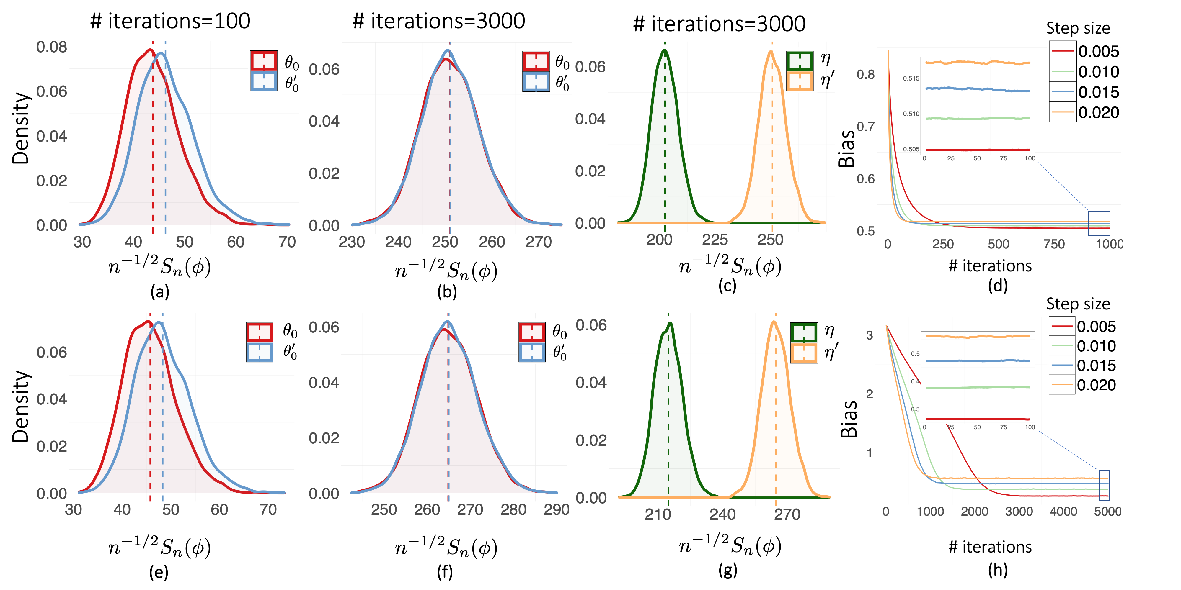
Figure 1: First and second rows correspond to non-convex examples in Sections 4.1.1 and 4.2.1, respectively. Figures (a,b), (e,f) show the density of n−1/2Sn(ϕ)=n−1/2∑k=1nϕ(θk(η))n^{-1/2}S_{n}(\phi)=n^{-1/2}\sum_{k=1}^{n}\phi(\theta^{(\eta)}_{k}) with different initializations (red, blue) for different number of iterations. Figures (c,g) show the same density with different step sizes. Figures (d,h) show the evolution of bias against the number of iterations.
Refer to caption
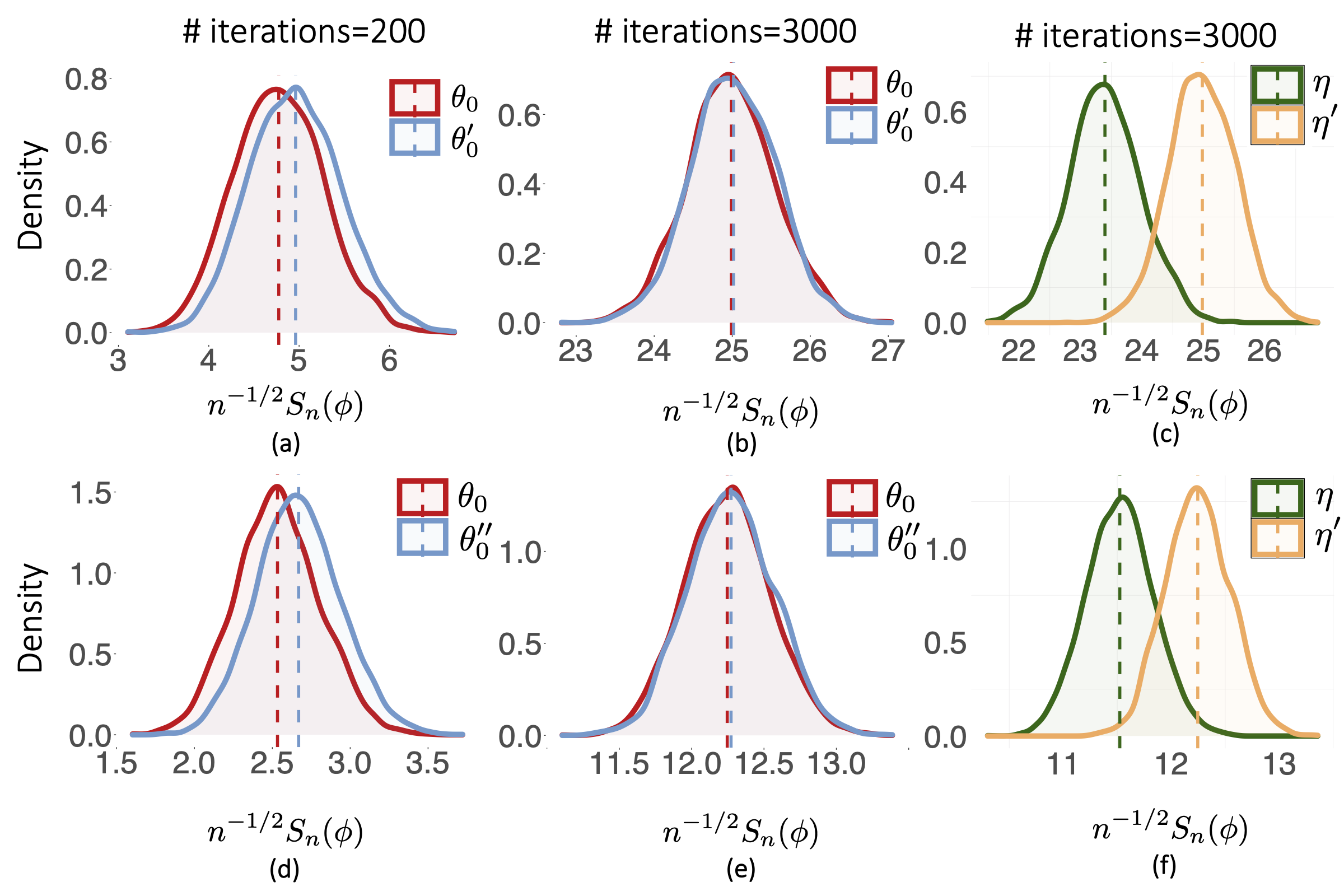
Figure 2: First and second rows correspond to non-convex examples in Sections 4.1.2 and 4.2.2, respectively. Figures (a,b), (e,f) show the density of n−1/2Sn(ϕ)=n−1/2∑k=1nϕ(θk(η))n^{-1/2}S_{n}(\phi)=n^{-1/2}\sum_{k=1}^{n}\phi(\theta^{(\eta)}_{k}) with different initializations (red, blue) for different number of iterations. Figures (c,g) show the same density with different step sizes.

Asymptotic normality: Fig. 1-(a,b,c,d) demonstrates the normality and the bias of SGD with heavy-tailed gradient noise distributed as Student-t (df=5\text{df}=5). Each plot has two density curves where red and blue curves in Fig. 1-(a,b) respectively correspond to initializations with θ0=(1,…,1)\theta_{0}=(1,\dots,1) and θ0′=(1.5,…,1.5)\theta^{\prime}_{0}=(1.5,\dots,1.5) with step size η=0.3\eta=0.3; green and orange curves in Fig. 1-c correspond to step sizes η=0.2\eta=0.2 and η′=0.3\eta^{\prime}=0.3 with initialization θ0\theta_{0}. All experiments are based on 4000 Monte Carlo runs. We observe in Fig. 1-a that different initializations have an early impact on the normality when the number of iterations is moderate. However, when SGD is run for a longer time, this effect is removed as in Fig. 1-b. Lastly, Fig.1-c demonstrates the effect of step size on the normality, where the means are different for different step sizes as they depend on the stationary distribution πη\pi_{\eta}. Indeed, the above results are not surprising. One can verify that the objective function (4.2) satisfies Assumptions 2.1 and 2.2. The above objective has the following gradient

∇f​(θ)=1m​∑i=1m𝐱i​(⟨𝐱i,θ⟩−yi)1+(yi−⟨𝐱i,θ⟩)2+λ​θ.\displaystyle\nabla f(\theta)=\frac{1}{m}\sum_{i=1}^{m}\frac{\mathbf{x}_{i}(\langle\mathbf{x}_{i},\,\theta\rangle-y_{i})}{1+(y_{i}-\langle\mathbf{x}_{i},\,\theta\rangle)^{2}}+\lambda\theta.

Because ‖∇f​(θ)‖≤(λmax​(1m​𝐗⊤​𝐗)+λ)​‖θ‖+1m​‖𝐗⊤​𝐲‖\|\nabla f(\theta)\|\leq\left(\lambda_{\text{max}}(\tfrac{1}{m}\mathbf{X}^{\top}\mathbf{X})+\lambda\right)\|\theta\|+\frac{1}{{m}}\|\mathbf{X}^{\top}\mathbf{y}\| by the triangle inequality and the fact that the denominator is lower bounded by 1, Assumption 2.1 holds. For Assumption 2.2, we write

⟨∇f​(θ),θ⟩=1m​∑i=1m(⟨𝐱i,θ⟩)2−yi​⟨𝐱i,θ⟩1+(yi−⟨𝐱i,θ⟩)2+λ​‖θ‖2≥−‖1m​𝐗⊤​𝐲‖​‖θ‖+λ​‖θ‖2,\displaystyle\langle\nabla f(\theta),\,\theta\rangle=\frac{1}{m}\sum_{i=1}^{m}\frac{(\langle\mathbf{x}_{i},\,\theta\rangle)^{2}-y_{i}\langle\mathbf{x}_{i},\,\theta\rangle}{1+(y_{i}-\langle\mathbf{x}_{i},\,\theta\rangle)^{2}}+\lambda\|\theta\|^{2}\geq-\big\|\frac{1}{m}\mathbf{X}^{\top}\mathbf{y}\big\|\|\theta\|+{\lambda}\|\theta\|^{2},

by Cauchy-Schwartz inequality. Next, using Young’s inequality −‖1m​𝐗⊤​𝐲‖​‖θ‖≥−1λ​‖1m​𝐗⊤​𝐲‖2−λ4​‖θ‖2,-\big\|\tfrac{1}{m}\mathbf{X}^{\top}\mathbf{y}\big\|\|\theta\|\!\geq\!-\frac{1}{\lambda}\big\|\tfrac{1}{m}\mathbf{X}^{\top}\mathbf{y}\big\|^{2}\!-\!\frac{\lambda}{4}\|\theta\|^{2}\,, Assumption 2.2 holds for α=λ/4\alpha\!=\!\lambda/4 and β=1λ​‖1m​𝐗⊤​𝐲‖2\beta\!=\!\frac{1}{\lambda}\big\|\tfrac{1}{m}\mathbf{X}^{\top}\mathbf{y}\big\|^{2}\!\!. Finally, the gradient noise has finite 4-th moment with support on ℝd\mathbb{R}^{d}; thus, Assumption 2.3 is satisfied, and Theorem 2.1 is applicable.

Bias: In order to demonstrate the bias behavior without speculation, one needs the global minimum θ∗\theta^{*} of the non-convex problem. Therefore, we simplify the problem (4.2) to another non-convex problem

f⁡(θ)≔12​log⁡(1+‖θ‖2)+λ2​‖θ‖2.\displaystyle f(\theta)\coloneqq\frac{1}{2}\log\bigl(1+\|\theta\|^{2}\bigr)+\frac{\lambda}{2}\|\theta\|^{2}\,. (4.3)

Notice that the general structure is the same, with no data, and θ∗\theta^{*} is known, i.e. θ∗=0\theta^{*}=0.

We choose the test function ϕ⁡(θ)=ϕ~∘f⁡(θ),\phi(\theta)=\tilde{\phi}\circ f(\theta), where ϕ~​(x)=1/(1+e−x)\tilde{\phi}(x)=1/(1+e^{-x}) is Lipschitz. Fig. 1-(d) demonstrates how the bias πη​(ϕ)−ϕ⁡(θ∗)\pi_{\eta}(\phi)-\phi(\theta^{*}) changes over iterations, where different curves correspond to different step sizes. We notice that larger step size provides fast initial decrease; yet the resulting asymptotic bias is larger which aligns with our theory. To verify assumptions, we compute the gradient and the Hessian respectively as

∇f​(θ)=θ1+‖θ‖2+λ​θ,and∇2f​(θ)=I1+‖θ‖2−2​θ​θ⊤(1+‖θ‖2)2+I​λ,\nabla f(\theta)=\frac{\theta}{1+\|\theta\|^{2}}+\lambda\theta,\qquad~\text{and}\qquad\nabla^{2}f(\theta)=\frac{I}{1+\|\theta\|^{2}}-\frac{2\theta\theta^{\top}}{(1+\|\theta\|^{2})^{2}}+I\lambda,

with II denoting the identity matrix. For small λ\lambda the above function is clearly non-convex. To see this, choose λ=0.1,u=θ/‖θ‖\lambda=0.1,u=\theta/\|\theta\| and note that ⟨u,∇2f​(θ)​u⟩<0\langle u,\,\nabla^{2}f(\theta)u\rangle<0 whenever 1.5≤‖θ‖≤21.5\leq\|\theta\|\leq 2. Also, note that

‖∇f​(θ)‖2=‖θ‖2​(λ+1/(1+‖θ‖2))2≥2​λ21+λ​{f⁡(θ)−f⁡(θ∗)}.\|\nabla f(\theta)\|^{2}=\|\theta\|^{2}\Bigl(\lambda+1/(1+\|\theta\|^{2})\Bigr)^{2}\geq\frac{2\lambda^{2}}{1+\lambda}\bigl\{f(\theta)-f(\theta^{*})\bigr\}.

Thus, Assumption 3.3 is satisfied for γ=2​λ21+λ\gamma=\frac{2\lambda^{2}}{1+\lambda} and g⁡(x)=γ​x2g(x)=\gamma x^{2}. Following the same steps in the regression setting, one can also verify Assumptions 2.1-2.3; hence, Theorem 3.2 can be applied.

4.1.2 Online Stochastic Gradient Descent

For our online SGD experiments, we use bk=2b_{k}=2, for all iterations kk to obtain the stochastic gradient. We also experimented with mk=10,50m_{k}=10,50 and observed similar behavior. The distribution of the random vector Z=(X,Y)∈ℝd+1Z=(X,Y)\in\mathbb{R}^{d+1}, is as follows: Each coordinate of the vector X∈ℝdX\in\mathbb{R}^{d}, is generated as Bernoulli​(±1)/d\text{Bernoulli}(\pm 1)/\sqrt{d} and given vector XX, the response Y∈ℝY\in\mathbb{R} is generated according to the linear model Y=⟨X,θtrue⟩+εY=\langle X,\,\theta_{\text{true}}\rangle+\varepsilon with each coordinate of θtrue∈ℝd\theta_{\text{true}}\in\mathbb{R}^{d} generated from Unif⁡(0,1),\operatorname{Unif}(0,1), and fixed, and ε∈ℝ\varepsilon\in\mathbb{R} is Student-t (df=10\text{df}=10) noise. We choose d=10,d=10, and set a burn-in period of size 100.

Asymptotic normality: Fig. 2-(a,b,c) demonstrates the normality of online SGD. Each plot has two density curves where red and blue curves in Fig. 2-(a,b) respectively correspond to initializations with θ0=(1,…,1)\theta_{0}=(1,\dots,1) and θ0′=(2.5,…,2.5)\theta^{{}^{\prime}}_{0}=(2.5,\dots,2.5) with step size η=0.3\eta=0.3; green and orange curves in Fig. 2-c correspond to step sizes η=0.2\eta=0.2 and η′=0.3\eta^{\prime}=0.3 with initialization θ0\theta_{0}. All experiments are based on 4000 Monte Carlo runs. We observe in Fig. 2-a that different initializations have an early impact on the normality when the number of iterations is moderate. However, when SGD is run for a longer time, this effect is removed as in Fig. 2-b. Lastly, Fig.2-c demonstrates the effect of step size on the normality, where the means are different for different step sizes as they depend on the stationary distribution πη\pi_{\eta}.

4.2 Regularized Blake-Zisserman MLE for corrupted linear regression

While the above example was based on linear-regression with heavy-tailed noise, we now consider the case of heavy-tailed regression with corrupted noise. In this setup, the noise model in linear regression is assumed to be Gaussian, but a fraction of the noise vectors are assumed to be corrupted in the sense that they are drawn from a uniform distribution. Such a scenario arises in visual reconstruction problems; see for example [BZ87] for details. In this case, defining the random vector Z:=(X,Y)Z:=(X,Y), the stochastic optimization problem in (1.3) is given by the expectation of the function

F⁡(Z,θ):=log⁡(ν+e−(Y−⟨X,θ⟩)2)+λ2​‖θ‖2,ν>0.\displaystyle F(Z,\theta):=\log\Bigl(\nu+e^{-(Y-\langle X,\,\theta\rangle)^{2}}\Bigr)+\frac{\lambda}{2}\|\theta\|^{2},~~~\nu>0. (4.4)

Similar the previous case, we also consider the finite-sum version: Given nn independent and identically distributed samples (𝐱i,yi)(\mathbf{x}_{i},y_{i}), it corresponds to minimizing the following objective function

f(θ)=−12​m∑i=1mlog(ν+e−(yi−⟨𝐱i,θ⟩)2)+λ2∥θ∥2,ν>0.\displaystyle f(\theta)=-\frac{1}{2m}\sum_{i=1}^{m}\log\Bigl(\nu+e^{-(y_{i}-\langle\mathbf{x}_{i},\,\theta\rangle)^{2}}\Bigr)+\frac{\lambda}{2}\|\theta\|^{2},~~~\nu>0\,.

4.2.1 Semi-stochastic Gradient Descent

In the experiments, we use the same setup and parameters as in Section 4.1.1.

Asymptotic normality: Fig 1-(e,f,g) demonstrates the asymptotic normality of the SGD with heavy-tailed gradient noise Student-t(df=6\text{df}=6). The experimental setup is the same as the previous example with the same values for θ0,θ0′,η,η′\theta_{0},\theta_{0}^{\prime},\eta,\eta^{\prime}. We observe the early impact of initialization in Fig 1-a, the clear normality in Fig. 1-b, and the effect of step size on CLT in Fig.1-c. These observations also align with our theory since this objective also satisfies our assumptions. Indeed, it has the gradient

∇f​(θ)\displaystyle\nabla f(\theta) =−1m∑i=1m𝐱i​(yi−⟨𝐱i,θ⟩)​e−(yi−⟨𝐱i,θ⟩)2ν+e−(yi−⟨𝐱i,θ⟩)2+λθ.\displaystyle=-\frac{1}{m}\sum_{i=1}^{m}\frac{\mathbf{x}_{i}\bigl(y_{i}-\langle\mathbf{x}_{i},\,\theta\rangle\bigr)e^{-(y_{i}-\langle\mathbf{x}_{i},\,\theta\rangle)^{2}}}{\nu+e^{-(y_{i}-\langle\mathbf{x}_{i},\,\theta\rangle)^{2}}}+\lambda\theta\,.

The triangle inequality yields

‖∇f​(θ)‖≤11+ν​‖1m​𝐗⊤​𝐲‖+(11+ν​λmax​(1m​𝐗⊤​𝐗)+λ)​‖θ‖,\|\nabla f(\theta)\|\leq\frac{1}{1+\nu}\big\|\tfrac{1}{m}\mathbf{X}^{\top}\mathbf{y}\big\|+\Big(\frac{1}{1+\nu}\lambda_{\text{max}}(\tfrac{1}{m}\mathbf{X}^{\top}\mathbf{X})+\lambda\Big)\|\theta\|,

which verifies Assumption 2.1. To verify the dissipativity assumption, we can write

⟨∇f(θ),θ⟩=⟨−1m∑i=1m𝐱i​(yi−⟨𝐱i,θ⟩)​e−(yi−⟨𝐱i,θ⟩)2ν+e−(yi−⟨𝐱i,θ⟩)2+λθ,θ⟩≥−11+ν∥1m𝐗⊤𝐲∥∥θ∥+λ∥θ∥2.\displaystyle\langle\nabla f(\theta),\,\theta\rangle=\langle-\frac{1}{m}\sum_{i=1}^{m}\frac{\mathbf{x}_{i}\bigl(y_{i}-\langle\mathbf{x}_{i},\,\theta\rangle\bigr)e^{-(y_{i}-\langle\mathbf{x}_{i},\,\theta\rangle)^{2}}}{\nu+e^{-(y_{i}-\langle\mathbf{x}_{i},\,\theta\rangle)^{2}}}+\lambda\theta,\,\theta\rangle\geq-\frac{1}{1+\nu}\big\|\tfrac{1}{m}\mathbf{X}^{\top}\mathbf{y}\big\|\|\theta\|+\lambda\|\theta\|^{2}\,.

The inequality follows from the triangle and Cauchy-Schwartz inequalities. Using Young’s inequality, we obtain

−11+ν​‖1m​𝐗⊤​𝐲‖​‖θ‖≥−1λ⁡(1+ν)​‖1m​𝐗⊤​𝐲‖2−λ4​(1+ν)​‖θ‖2,-\frac{1}{1+\nu}\big\|\tfrac{1}{m}\mathbf{X}^{\top}\mathbf{y}\big\|\|\theta\|\geq-\frac{1}{\lambda(1+\nu)}\big\|\tfrac{1}{m}\mathbf{X}^{\top}\mathbf{y}\big\|^{2}-\frac{\lambda}{4(1+\nu)}\|\theta\|^{2},

which shows that the above function is dissipative for α=λ/2\alpha=\lambda/2 and β=12​λ​(1+ν)2​‖1m​𝐗⊤​𝐲‖2\beta=\frac{1}{2\lambda(1+\nu)^{2}}\big\|\tfrac{1}{m}\mathbf{X}^{\top}\mathbf{y}\big\|^{2}; thus, Assumption 2.2 holds.

Bias: Similar to the previous example, we simplify the problem so that we can compute the bias πη​(ϕ)−ϕ⁡(θ∗)\pi_{\eta}(\phi)-\phi(\theta^{*}). We consider the function

f⁡(θ)≔−12​log⁡(ν+e−‖θ‖2)+λ2​‖θ‖2,ν>0.\displaystyle f(\theta)\coloneqq-\frac{1}{2}\log\big(\nu+e^{-\|\theta\|^{2}}\big)+\frac{\lambda}{2}\|\theta\|^{2},~~~\nu>0\,.

We observe in Fig.1-h that smaller step sizes lead to smaller asymptotic bias. To verify that this can be predicted from our theory, we write the gradient and the Hessian respectively, as

∇f​(θ)=θ1+ν​e‖θ‖2+λ​θand∇2f​(θ)=I1+ν​e‖θ‖2−2​ν​e‖θ‖2(1+ν​e‖θ‖2)2​θ​θ⊤+λ​I.\nabla f(\theta)=\frac{\theta}{1+\nu e^{\|\theta\|^{2}}}+\lambda\theta~\qquad\text{and}~\qquad\nabla^{2}f(\theta)=\frac{I}{1+\nu e^{\|\theta\|^{2}}}-\frac{2\nu e^{\|\theta\|^{2}}}{(1+\nu e^{\|\theta\|^{2}})^{2}}\theta\theta^{\top}+\lambda I.

First, note that the Hessian can have negative eigenvalues for small values of λ\lambda. For example, for ν=1\nu=1, λ=0.1\lambda=0.1, and the unit direction u=θ/‖θ‖u=\theta/\|\theta\|, we have ⟨u,∇2f​(θ)​u⟩<0\langle u,\,\nabla^{2}f(\theta)u\rangle<0 for 1≤‖θ‖2≤21\leq\|\theta\|^{2}\leq 2; thus the function is non-convex. But we also have

⟨∇f​(θ),θ⟩=‖θ‖2​(λ+1/(1+ν​e‖θ‖2))≥(λ+1/(1+ν​eR2))​‖θ‖2\displaystyle\langle\nabla f(\theta),\,\theta\rangle=\|\theta\|^{2}\Big(\lambda+1/\big(1+\nu e^{\|\theta\|^{2}}\big)\Big)\geq\Big(\lambda+1/\big(1+\nu e^{R^{2}}\big)\Big)\|\theta\|^{2}

for ‖θ‖≤R\|\theta\|\leq R and ⟨∇f​(θ),θ⟩≥λ​‖θ‖2\langle\nabla f(\theta),\,\theta\rangle\geq\lambda\|\theta\|^{2} for ‖θ‖2>R\|\theta\|^{2}>R; thus, Assumption 3.2 is satisfied for α=λ\alpha=\lambda, and any β≥0\beta\geq 0 and g⁡(x)=(λ+1/(1+ν​eR2))​x2g(x)=\Big(\lambda+1/\big(1+\nu e^{R^{2}}\big)\Big)x^{2}. Following the same steps in the previous example, one can also verify Assumptions 2.1-2.3; therefore, Theorem 3.1 follows.

4.2.2 Online Stochastic Gradient Descent

In the experiments, we use the same setup as in Section 4.1.2.

Asymptotic normality: Fig. 2-(d,e,f) demonstrates the normality of online SGD. Each plot has two density curves where red and blue curves in Fig. 2-(d,e) respectively correspond to initializations with θ0=(1,…,1)\theta_{0}=(1,\dots,1) and θ0′′=(1.5,…,1.5)\theta^{{}^{\prime\prime}}_{0}=(1.5,\dots,1.5) with step size η=0.3\eta=0.3; green and orange curves in Fig. 2-c correspond to step sizes η=0.2\eta=0.2 and η′=0.3\eta^{\prime}=0.3 with initialization θ0\theta_{0}. All experiments are based on 4000 Monte Carlo runs. We observe in Fig. 2-d that different initializations have an early impact on the normality when the number of iterations are moderate. However, when SGD is run for a longer time, this effect is removed as in Fig. 2-e. Lastly, Fig.2-f demonstrates the effect of step size on the normality, where the means are different for different step sizes as they depend on the stationary distribution πη\pi_{\eta}.

5 Discussions

By leveraging the connection between constant step size SGD and Markov chains [DDB19], we provided theoretical results characterizing the bias and the fluctuations of constant step size SGD for non-convex and non-smooth optimization which arises frequently in modern statistical learning.

Estimating the Asymptotic Variance: As discussed in Section 2, in order for using the established CLT to compute confidence intervals in practice, the population expectation πη​(ϕ)\pi_{\eta}(\phi) and asymptotic variance σπη2​(ϕ)\sigma^{2}_{\pi_{\eta}}(\phi) have to be estimated. We suggest the following three ways to do so:

  • •

    Estimate them based on sample average of a single trajectory of SGD iterates, i.e., the mean πη​(ϕ)\pi_{\eta}(\phi) is estimated as n−1​∑k=0n−1ϕ⁡(θk(η))n^{-1}\sum_{k=0}^{n-1}\phi\big(\theta^{(\eta)}_{k}\big) and the variance σπη2​(ϕ)\sigma^{2}_{\pi_{\eta}}(\phi) by adopting the online approach of [ZCW20] to the constant step size setting.

  • •

    First run NN parallel SGD trajectories and compute the average of each trajectory, to obtain NN independent observations from the stationary distribution πη\pi_{\eta}. Next, use the NN observations to compute the sample mean and the sample variance estimators for πη​(ϕ)\pi_{\eta}(\phi) and σπη2​(ϕ)\sigma^{2}_{\pi_{\eta}}(\phi).

  • •

    Leverage the online bootstrap and variance estimation approaches proposed in [FXY18, SZ18, CLT+20] for the constant step size SGD setting in order to obtain estimates for πη​(ϕ)\pi_{\eta}(\phi) and σπη2​(ϕ)\sigma^{2}_{\pi_{\eta}}(\phi).

A theoretical investigation on the relative merits of the above approaches is left as future work.

Acknowledgements

MAE is partially funded by NSERC Grant [2019-06167], Connaught New Researcher Award, CIFAR AI Chairs program, and CIFAR AI Catalyst grant. KB is partially supported by a seed grant from the Center for Data Science and Artificial Intelligence Research, UC Davis. SV is partially supported by a discovery grant from NSERC of Canada and a Connaught New Researcher Award. The authors thank Yichen Zhang for helpful comments on an earlier version of this manuscript.

References

  • [ABE19] Andreas Anastasiou, Krishnakumar Balasubramanian, and Murat A Erdogdu, Normal approximation for stochastic gradient descent via non-asymptotic rates of martingale clt, Conference on Learning Theory, 2019, pp. 115–137.
  • [AMP00] Rafik Aguech, Eric Moulines, and Pierre Priouret, On a perturbation approach for the analysis of stochastic tracking algorithms, SIAM Journal on Control and Optimization 39 (2000), no. 3, 872–899.
  • [BDMP17] Nicolas Brosse, Alain Durmus, Éric Moulines, and Marcelo Pereyra, Sampling from a log-concave distribution with compact support with proximal langevin monte carlo, COLT, 2017.
  • [BEL18] Sébastien Bubeck, Ronen Eldan, and Joseph Lehec, Sampling from a log-concave distribution with projected langevin monte carlo, Discrete & Computational Geometry (2018).
  • [Ben96] Michel Benaim, A dynamical system approach to stochastic approximations, SIAM Journal on Control and Optimization 34 (1996), no. 2, 437–472.
  • [BH18] Lukas Balles and Philipp Hennig, Dissecting adam: The sign, magnitude and variance of stochastic gradients, International Conference on Machine Learning, 2018, pp. 404–413.
  • [BVB16] Nicolas Boumal, Vlad Voroninski, and Afonso Bandeira, The non-convex burer-monteiro approach works on smooth semidefinite programs, Advances in Neural Information Processing Systems, 2016, pp. 2757–2765.
  • [BZ87] Andrew Blake and Andrew Zisserman, Visual reconstruction, 1987.
  • [CCAY+18] Xiang Cheng, Niladri S Chatterji, Yasin Abbasi-Yadkori, Peter L Bartlett, and Michael I Jordan, Sharp convergence rates for langevin dynamics in the nonconvex setting, arXiv preprint arXiv:1805.01648 (2018).
  • [CCBJ17] Xiang Cheng, Niladri S Chatterji, Peter L Bartlett, and Michael I Jordan, Underdamped langevin mcmc: A non-asymptotic analysis, arXiv preprint arXiv:1707.03663 (2017).
  • [Chu54] Kai Lai Chung, On a stochastic approximation method, The Annals of Mathematical Statistics (1954), 463–483.
  • [CLC19] Yuejie Chi, Yue M Lu, and Yuxin Chen, Nonconvex optimization meets low-rank matrix factorization: An overview, IEEE Transactions on Signal Processing 67 (2019), no. 20, 5239–5269.
  • [CLPC19] Changxiao Cai, Gen Li, H Vincent Poor, and Yuxin Chen, Nonconvex low-rank tensor completion from noisy data, Advances in Neural Information Processing Systems, 2019, pp. 1861–1872.
  • [CLT+20] Xi Chen, Jason D Lee, Xin T Tong, Yichen Zhang, et al., Statistical inference for model parameters in stochastic gradient descent, The Annals of Statistics 48 (2020), no. 1, 251–273.
  • [CT18] Jerry Chee and Panos Toulis, Convergence diagnostics for stochastic gradient descent with constant learning rate, International Conference on Artificial Intelligence and Statistics, 2018, pp. 1476–1485.
  • [Dal17] Arnak S Dalalyan, Theoretical guarantees for approximate sampling from smooth and log-concave densities, Journal of the Royal Statistical Society: Series B (Statistical Methodology) 79 (2017), no. 3, 651–676.
  • [DCLZ19] Zhiyan Ding, Yiding Chen, Qin Li, and Xiaojin Zhu, Error lower bounds of constant step-size stochastic gradient descent, arXiv preprint arXiv:1910.08212 (2019).
  • [DCWY18] Raaz Dwivedi, Yuansi Chen, Martin J Wainwright, and Bin Yu, Log-concave sampling: Metropolis-hastings algorithms are fast!, arXiv preprint arXiv:1801.02309 (2018).
  • [DDB19] Aymeric Dieuleveut, Alain Durmus, and Francis Bach, Bridging the gap between constant step size stochastic gradient descent and markov chains, The Annals of Statistics (to appear) (2019).
  • [DK17] Arnak S Dalalyan and Avetik G Karagulyan, User-friendly guarantees for the langevin monte carlo with inaccurate gradient, arXiv preprint arXiv:1710.00095 (2017).
  • [DM17] Alain Durmus and Eric Moulines, Nonasymptotic convergence analysis for the unadjusted langevin algorithm, The Annals of Applied Probability 27 (2017), no. 3, 1551–1587.
  • [DMPS18] Randal Douc, Eric Moulines, Pierre Priouret, and Philippe Soulier, Markov chains, Springer, 2018.
  • [DR18] John Duchi and Feng Ruan, Asymptotic optimality in stochastic optimization, Arxiv Preprint (2018).
  • [DRD18] Arnak S Dalalyan and Lionel Riou-Durand, On sampling from a log-concave density using kinetic langevin diffusions, arXiv preprint arXiv:1807.09382 (2018).
  • [DYJG17] Soham De, Abhay Yadav, David Jacobs, and Tom Goldstein, Automated inference with adaptive batches, Artificial Intelligence and Statistics, 2017, pp. 1504–1513.
  • [EH20] Murat A Erdogdu and Rasa Hosseinzadeh, On the convergence of langevin monte carlo: The interplay between tail growth and smoothness, arXiv preprint arXiv:2005.13097 (2020).
  • [EMS18] Murat A Erdogdu, Lester Mackey, and Ohad Shamir, Global non-convex optimization with discretized diffusions, Advances in Neural Information Processing Systems, 2018, pp. 9671–9680.
  • [EvdG18] Andreas Elsener and Sara van de Geer, Sharp oracle inequalities for stationary points of nonconvex penalized m-estimators, IEEE Transactions on Information Theory 65 (2018), no. 3, 1452–1472.
  • [Fab68] Vaclav Fabian, On asymptotic normality in stochastic approximation, The Annals of Mathematical Statistics 39 (1968), no. 4, 1327–1332.
  • [FD82] DA Freedman and P Diaconis, On inconsistent mm-estimators, The Annals of Statistics 10 (1982), no. 2, 454–461.
  • [FLLZ18] Cong Fang, Chris Junchi Li, Zhouchen Lin, and Tong Zhang, Spider: Near-optimal non-convex optimization via stochastic path-integrated differential estimator, Advances in Neural Information Processing Systems, 2018, pp. 689–699.
  • [FP99] Jean-Claude Fort and Gilles Pages, Asymptotic behavior of a markovian stochastic algorithm with constant step, SIAM journal on control and optimization 37 (1999), no. 5, 1456–1482.
  • [FXY18] Yixin Fang, Jinfeng Xu, and Lei Yang, Online bootstrap confidence intervals for the stochastic gradient descent estimator, The Journal of Machine Learning Research 19 (2018), no. 1, 3053–3073.
  • [FY17] Jianqing Fan and Qiwei Yao, The elements of financial econometrics, Cambridge University Press, 2017.
  • [GBC16] Ian Goodfellow, Yoshua Bengio, and Aaron Courville, Deep learning, MIT press, 2016.
  • [Gey94] Charles J Geyer, On the asymptotics of constrained mm-estimation, The Annals of Statistics 22 (1994), no. 4, 1993–2010.
  • [GHJY15] Rong Ge, Furong Huang, Chi Jin, and Yang Yuan, Escaping from saddle points - online stochastic gradient for tensor decomposition, Conference on Learning Theory, 2015, pp. 797–842.
  • [GL13] Saeed Ghadimi and Guanghui Lan, Stochastic first-and zeroth-order methods for nonconvex stochastic programming, SIAM Journal on Optimization 23 (2013), no. 4, 2341–2368.
  • [GLCY16] Bin Gao, Xin Liu, Xiaojun Chen, and Ya-xiang Yuan, On the {\{\\backslashL}\} ojasiewicz exponent of the quadratic sphere constrained optimization problem, arXiv preprint arXiv:1611.08781 (2016).
  • [GLM16] Rong Ge, Jason D Lee, and Tengyu Ma, Matrix completion has no spurious local minimum, Advances in Neural Information Processing Systems, 2016, pp. 2973–2981.
  • [Hub04] Peter J Huber, Robust statistics, vol. 523, John Wiley & Sons, 2004.
  • [JGN+17] Chi Jin, Rong Ge, Praneeth Netrapalli, Sham M Kakade, and Michael I Jordan, How to escape saddle points efficiently, Proceedings of the 34th International Conference on Machine Learning-Volume 70, JMLR. org, 2017, pp. 1724–1732.
  • [JK17] Prateek Jain and Purushottam Kar, Non-convex optimization for machine learning, Foundations and Trends® in Machine Learning 10 (2017), no. 3-4, 142–336.
  • [Kaw16] Kenji Kawaguchi, Deep learning without poor local minima, Advances in neural information processing systems, 2016, pp. 586–594.
  • [Kif88] Yuri Kifer, Random perturbations of dynamical systems, Nonlinear Problems in Future Particle Accelerators. World Scientific (1988), 189.
  • [KNS16] Hamed Karimi, Julie Nutini, and Mark Schmidt, Linear convergence of gradient and proximal-gradient methods under the polyak-łojasiewicz condition, Joint European Conference on Machine Learning and Knowledge Discovery in Databases, Springer, 2016, pp. 795–811.
  • [LLM18] Guillaume Lecué, Matthieu Lerasle, and Timothée Mathieu, Robust classification via mom minimization, arXiv preprint arXiv:1808.03106 (2018).
  • [Loh17] Po-Ling Loh, Statistical consistency and asymptotic normality for high-dimensional robust mm-estimators, The Annals of Statistics 45 (2017), no. 2, 866–896.
  • [LWME19] Xuechen Li, Yi Wu, Lester Mackey, and Murat A Erdogdu, Stochastic runge-kutta accelerates langevin monte carlo and beyond, Advances in Neural Information Processing Systems, 2019, pp. 7748–7760.
  • [MB11] Eric Moulines and Francis R Bach, Non-asymptotic analysis of stochastic approximation algorithms for machine learning, Advances in Neural Information Processing Systems, 2011, pp. 451–459.
  • [MBB18] Siyuan Ma, Raef Bassily, and Mikhail Belkin, The power of interpolation: Understanding the effectiveness of sgd in modern over-parametrized learning, International Conference on Machine Learning, 2018, pp. 3325–3334.
  • [MBM18] Song Mei, Yu Bai, and Andrea Montanari, The landscape of empirical risk for nonconvex losses, The Annals of Statistics 46 (2018), no. 6A, 2747–2774.
  • [MIG+19] Wesley J Maddox, Pavel Izmailov, Timur Garipov, Dmitry P Vetrov, and Andrew Gordon Wilson, A simple baseline for bayesian uncertainty in deep learning, Advances in Neural Information Processing Systems, 2019, pp. 13132–13143.
  • [MMMO17] Song Mei, Theodor Misiakiewicz, Andrea Montanari, and Roberto Imbuzeiro Oliveira, Solving sdps for synchronization and maxcut problems via the grothendieck inequality, Conference on Learning Theory, 2017, pp. 1476–1515.
  • [MSH02] Jonathan C Mattingly, Andrew M Stuart, and Desmond J Higham, Ergodicity for sdes and approximations: locally lipschitz vector fields and degenerate noise, Stochastic processes and their applications 101 (2002), no. 2, 185–232.
  • [MT12] Sean P Meyn and Richard L Tweedie, Markov chains and stochastic stability, Springer Science & Business Media, 2012.
  • [NP06] Yurii Nesterov and Boris T Polyak, Cubic regularization of newton method and its global performance, Mathematical Programming 108 (2006), no. 1, 177–205.
  • [NWS14] Deanna Needell, Rachel Ward, and Nati Srebro, Stochastic gradient descent, weighted sampling, and the randomized kaczmarz algorithm, Advances in neural information processing systems, 2014, pp. 1017–1025.
  • [PJ92] Boris T Polyak and Anatoli B Juditsky, Acceleration of stochastic approximation by averaging, SIAM Journal on Control and Optimization 30 (1992), no. 4, 838–855.
  • [PV98] P Priouret and A Yu Veretenikov, A remark on the stability of the lms tracking algorithm, Stochastic analysis and applications 16 (1998), no. 1, 119–129.
  • [QCLP19] Zhengling Qi, Ying Cui, Yufeng Liu, and Jong-Shi Pang, Statistical analysis of stationary solutions of coupled nonconvex nonsmooth empirical risk minimization, arXiv preprint arXiv:1910.02488 (2019).
  • [RM51] Herbert Robbins and Sutton Monro, A stochastic approximation method, The annals of mathematical statistics (1951), 400–407.
  • [RRT17] Maxim Raginsky, Alexander Rakhlin, and Matus Telgarsky, Non-convex learning via stochastic gradient langevin dynamics: a nonasymptotic analysis, Conference on Learning Theory, 2017, pp. 1674–1703.
  • [Rup88] David Ruppert, Efficient estimations from a slowly convergent robbins-monro process, Tech. report, Cornell University Operations Research and Industrial Engineering, 1988.
  • [Sac58] Jerome Sacks, Asymptotic distribution of stochastic approximation procedures, The Annals of Mathematical Statistics 29 (1958), no. 2, 373–405.
  • [Sha89] Alexander Shapiro, Asymptotic properties of statistical estimators in stochastic programming, The Annals of Statistics 17 (1989), no. 2, 841–858.
  • [Sha00]   , On the asymptotics of constrained local m-estimators, Annals of statistics (2000), 948–960.
  • [SL19] Ruoqi Shen and Yin Tat Lee, The randomized midpoint method for log-concave sampling, Advances in Neural Information Processing Systems, 2019, pp. 2098–2109.
  • [SR13] Mark Schmidt and Nicolas Le Roux, Fast convergence of stochastic gradient descent under a strong growth condition, arXiv preprint arXiv:1308.6370 (2013).
  • [SZ18] Weijie Su and Yuancheng Zhu, Statistical inference for online learning and stochastic approximation via hierarchical incremental gradient descent, arXiv preprint arXiv:1802.04876 (2018).
  • [TA17] Panos Toulis and Edoardo M Airoldi, Asymptotic and finite-sample properties of estimators based on stochastic gradients, The Annals of Statistics 45 (2017), no. 4, 1694–1727.
  • [TFBJ18] Nilesh Tripuraneni, Nicolas Flammarion, Francis Bach, and Michael I Jordan, Averaging stochastic gradient descent on riemannian manifolds, arXiv preprint arXiv:1802.09128 (2018).
  • [TSJ+18] Nilesh Tripuraneni, Mitchell Stern, Chi Jin, Jeffrey Regier, and Michael I Jordan, Stochastic cubic regularization for fast nonconvex optimization, Advances in neural information processing systems, 2018, pp. 2899–2908.
  • [TV19] Yan Shuo Tan and Roman Vershynin, Online stochastic gradient descent with arbitrary initialization solves non-smooth, non-convex phase retrieval, arXiv preprint arXiv:1910.12837 (2019).
  • [VBS19] Sharan Vaswani, Francis Bach, and Mark Schmidt, Fast and faster convergence of sgd for over-parameterized models and an accelerated perceptron, The 22nd International Conference on Artificial Intelligence and Statistics, 2019, pp. 1195–1204.
  • [WRS+17] Ashia C Wilson, Rebecca Roelofs, Mitchell Stern, Nati Srebro, and Benjamin Recht, The marginal value of adaptive gradient methods in machine learning, Advances in Neural Information Processing Systems, 2017, pp. 4148–4158.
  • [XCZG18] Pan Xu, Jinghui Chen, Difan Zou, and Quanquan Gu, Global convergence of langevin dynamics based algorithms for nonconvex optimization, Advances in Neural Information Processing Systems, 2018, pp. 3122–3133.
  • [XYZ19] Dong Xia, Ming Yuan, and Cun-Hui Zhang, Statistically optimal and computationally efficient low rank tensor completion from noisy entries, The Annals of Statistics (to appear) (2019).
  • [ZCW20] Wanrong Zhu, Xi Chen, and Wei Biao Wu, A fully online approach for covariance matrices estimation of stochastic gradient descent solutions, arXiv preprint arXiv:2002.03979 (2020).

Appendix A Proofs for Sections 2 and 3

A.1 Preliminaries and Additional Notations

Note that the sequence of iterates {θk(η)}k≥0\{\theta^{(\eta)}_{k}\}_{k\geq 0} is a homogeneous Markov chain [DDB19]. We denote the (sub-)σ\sigma-algebra (of ℱ\mathcal{F}) of events up to and including the kk-th iteration as ℱk.\mathcal{F}_{k}. By definition, the discrete-time stochastic process defined in (1.2) is adapted to its natural filtration {ℱk}k≥0\{\mathcal{F}_{k}\}_{k\geq 0}. We denote the Markov kernel on (ℝd,ℬ⁡(ℝd))(\mathbb{R}^{d},\mathcal{B}(\mathbb{R}^{d})) associated with SGD iterates (1.2) by PP with

P⁡(θk(η),A)=ℙ⁡(θk+1(η)∈A|θk(η))​ℙ−a.s.,∀A∈ℬ⁡(ℝd),k≥0.P(\theta^{(\eta)}_{k},A)=\mathbb{P}(\theta^{(\eta)}_{k+1}\in A|\theta^{(\eta)}_{k})~~\mathbb{P}-a.s.,~~~\forall A\in\mathcal{B}(\mathbb{R}^{d}),k\geq 0\,.

Define the kk-th power of this kernel iteratively: define P1:=P,P^{1}:=P, and for k≥1,k\geq 1, for all θ~∈ℝd\tilde{\theta}\in\mathbb{R}^{d} and A∈ℬ⁡(ℝd),A\in\mathcal{B}(\mathbb{R}^{d}), define

Pk+1​(θ~,A):=∫ℝdP⁡(θ~,𝑑θ)​Pk​(θ,A).P^{k+1}(\tilde{\theta},A):=\int_{\mathbb{R}^{d}}P(\tilde{\theta},d\theta)P^{k}(\theta,A)\,.

For any function ϕ:ℝd→ℝ\phi:\mathbb{R}^{d}\to\mathbb{R} and k≥0,k\geq 0, define the measurable function Pk​ϕ​(θ):ℝd→ℝP^{k}\phi(\theta):\mathbb{R}^{d}\to\mathbb{R} for all θ∈ℝd\theta\in\mathbb{R}^{d} via

Pk​ϕ​(θ)=∫ϕ⁡(θ~)​Pk​(θ,𝑑θ~).P^{k}\phi(\theta)=\int\phi(\tilde{\theta})P^{k}(\theta,d\tilde{\theta})\,.

Given the LϕL_{\phi}-Lipschitz function ϕ:ℝd→ℝ\phi:\mathbb{R}^{d}\to\mathbb{R} and the expectation of ϕ\phi under the stationary measure πη,\pi_{\eta}, define the function hh as

h:ℝd\displaystyle h:\mathbb{R}^{d} →ℝ\displaystyle\to\mathbb{R}
θ\displaystyle\theta ↦ϕ⁡(θ)−πη​(ϕ).\displaystyle\mapsto\phi(\theta)-\pi_{\eta}(\phi)\,.

Note that πη​(h)=0\pi_{\eta}(h)=0 and hh is LϕL_{\phi}-Lipschitz. Define the partial sum Sn​(ϕ):=∑k=0n−1h⁡(θk(η)).S_{n}(\phi):=\sum_{k=0}^{n-1}h(\theta^{(\eta)}_{k}). Moreover, we define

θ¯η:=∫ℝdθ​d​πη​(θ).\bar{\theta}_{\eta}:=\int_{\mathbb{R}^{d}}\theta d\pi_{\eta}(\theta)\,.

A.2 Proofs of Proposition 2.1 and Theorem 2.1

We start with some preliminary results required to prove the CLT.

Lemma A.1.

Under Assumptions 2.1-2.3, it holds for any η∈(0,α−(α2−(3​L2+Lξ))∨03​L2+Lξ)\eta\in\left(0,\frac{\alpha-\sqrt{(\alpha^{2}-{(3L^{2}+L_{\xi})})\vee 0}}{{3L^{2}+L_{\xi}}}\right) and any fixed initial point θ0(η)=θ0∈ℝd\theta^{(\eta)}_{0}=\theta_{0}\in\mathbb{R}^{d} that

𝔼⁡[‖θk+1(η)‖2+1|ℱk]≤α†​(‖θk(η)‖2+1)+β†.\mathbb{E}[\,\|\theta^{(\eta)}_{k+1}\|^{2}+1|\mathcal{F}_{k}]\leq\alpha_{\dagger}(\,\|\theta^{(\eta)}_{k}\|^{2}+1)+\beta_{\dagger}\,.

Here, α†∈(0,1)\alpha_{\dagger}\in(0,1) and β†∈(0,∞)\beta_{\dagger}\in(0,\infty) are constants depending on η.\eta. The explicit formulas of α†,β†\alpha_{\dagger},\beta_{\dagger} are given in the proof.

Proof of Lemma A.1.

Define Uη:=α−max⁡{α2−(3​L2+Lξ),0}3​L2+Lξ.U_{\eta}:=\frac{\alpha-\sqrt{\max\{\alpha^{2}-{(3L^{2}+L_{\xi})},0\}}}{{3L^{2}+L_{\xi}}}. Given η∈(0,Uη),\eta\in(0,U_{\eta}), define

α†=1+η2​(3​L2+Lξ)−2​η​α\alpha_{\dagger}=1+\eta^{2}{(3L^{2}+L_{\xi})}-2\eta\alpha

and note that with this definition α†∈(0,1)\alpha_{\dagger}\in(0,1) whenever η∈(0,Uη)\eta\in(0,U_{\eta}). Then, with η,α†\eta,\alpha_{\dagger}, and the fixed initial point θ0(η)=θ0∈ℝd,\theta^{(\eta)}_{0}=\theta_{0}\in\mathbb{R}^{d}, we set

β†:=κ⁡(α†1/2−α†),\beta_{\dagger}:={\kappa(\alpha_{\dagger}^{1/2}-\alpha_{\dagger})}\,,

where

κ:=\displaystyle\kappa:= 4​η​(α+β)+12​η2​L2α†1/2−α†​⋁1.\displaystyle\frac{4\eta(\alpha+\beta)+12\eta^{2}L^{2}}{{\alpha_{\dagger}^{1/2}-\alpha_{\dagger}}}\bigvee 1\,.

It follows that β†>0.\beta_{\dagger}>0. Note that

𝔼⁡[1+‖θk+1(η)‖2|ℱk]\displaystyle\mathbb{E}[1+\|\theta^{(\eta)}_{k+1}\|^{2}|\mathcal{F}_{k}]
=\displaystyle= 𝔼⁡[1+‖θk(η)−η⁡(∇f​(θk(η))+ξk+1​(θk(η)))‖2|ℱk]\displaystyle\mathbb{E}[1+\|\theta^{(\eta)}_{k}-\eta\bigl(\nabla f(\theta^{(\eta)}_{k})+{\xi_{k+1}(\theta^{(\eta)}_{k})}\bigr)\|^{2}|\mathcal{F}_{k}]
=\displaystyle= 1+𝔼⁡[‖θk(η)‖2+η2​‖∇f​(θk(η))‖2+η2​‖ξk+1​(θk(η))‖2−2​η​⟨θk(η),∇f​(θk(η))⟩|ℱk].\displaystyle 1+\mathbb{E}\bigl[\,\|\theta^{(\eta)}_{k}\|^{2}+\eta^{2}\,\|\nabla f(\theta^{(\eta)}_{k})\|^{2}+\eta^{2}\,\|{\xi_{k+1}(\theta^{(\eta)}_{k})}\|^{2}-2\eta\langle\theta^{(\eta)}_{k},\,\nabla f(\theta^{(\eta)}_{k})\rangle|\mathcal{F}_{k}\bigr]\,.

The last step follows from the Assumption 2.3. By Assumption 2.1, we have

‖∇f​(θk(η))‖2≤L2​(1+‖θk(η)‖)2.\|\nabla f(\theta^{(\eta)}_{k})\|^{2}\leq L^{2}(1+\|\theta^{(\eta)}_{k}\|)^{2}\,.

Squaring both sides and using the fact that (1+‖θk(η)‖)2≤3​(‖θk(η)‖2+3)(1+\|\theta^{(\eta)}_{k}\|)^{2}\leq 3(\,\|\theta^{(\eta)}_{k}\|^{2}+3) gives

‖∇f​(θk(η))‖2≤3​L2​(‖θk(η)‖2+3).\|\nabla f(\theta^{(\eta)}_{k})\|^{2}\leq 3L^{2}(\,\|\theta^{(\eta)}_{k}\|^{2}+3)\,.

By Assumption 2.2, we obtain

⟨θk(η),∇f​(θk(η))⟩≥α​‖θk(η)‖2−β.\langle\theta^{(\eta)}_{k},\,\nabla f(\theta^{(\eta)}_{k})\rangle\geq\alpha\,\|\theta^{(\eta)}_{k}\|^{2}-\beta\,.

By Assumption 2.3, it holds that

𝔼⁡[‖ξk+1​(θk(η))‖2|ℱk]≤Lξ​(1+‖θk(η)‖2).{\mathbb{E}[\,\|\xi_{k+1}(\theta^{(\eta)}_{k})\|^{2}|\mathcal{F}_{k}]\leq L_{\xi}(1+\|\theta^{(\eta)}_{k}\|^{2})\,.}

Plugging the previous three inequalities into the first display provides us with

𝔼⁡[1+‖θk+1(η)‖2|ℱk]≤1+9​η2​L2+η2​Lξ+2​η​β+(1+3​η2​L2+η2​Lξ−2​η​α)​‖θk(η)‖2.\mathbb{E}[1+\|\theta^{(\eta)}_{k+1}\|^{2}|\mathcal{F}_{k}]\leq 1+9\eta^{2}L^{2}+{\eta^{2}L_{\xi}}+2\eta\beta+(1+3\eta^{2}L^{2}+{\eta^{2}L_{\xi}}-2\eta\alpha)\,\|\theta^{(\eta)}_{k}\|^{2}\,. (A.1)

Recall that α†=1+η2​(3​L2+Lξ)−2​η​α.\alpha_{\dagger}=1+\eta^{2}{(3L^{2}+L_{\xi})}-2\eta\alpha. Plugging α†\alpha_{\dagger} back into the previous display yields

𝔼⁡[‖θk+1(η)‖2+1|ℱk]≤α†​(‖θk(η)‖2+1)+2​η​(α+β)+6​η2​L2.\mathbb{E}[\,\|\theta^{(\eta)}_{k+1}\|^{2}+1|\mathcal{F}_{k}]\leq\alpha_{\dagger}(\,\|\theta^{(\eta)}_{k}\|^{2}+1)+2\eta(\alpha+\beta)+6\eta^{2}L^{2}\,. (A.2)

Note that β†=κ⁡(α†1/2−α†),\beta_{\dagger}={\kappa(\alpha_{\dagger}^{1/2}-\alpha_{\dagger})}, where

κ≥4​η​(α+β)+12​η2​L2α†1/2−α†.\kappa\geq\frac{4\eta(\alpha+\beta)+12\eta^{2}L^{2}}{{\alpha_{\dagger}^{1/2}-\alpha_{\dagger}}}\,.

It then follows that 𝔼⁡[‖θk+1(η)‖2+1|ℱk]≤α†​(‖θk(η)‖2+1)+β†\mathbb{E}[\,\|\theta^{(\eta)}_{k+1}\|^{2}+1|\mathcal{F}_{k}]\leq\alpha_{\dagger}(\,\|\theta^{(\eta)}_{k}\|^{2}+1)+\beta_{\dagger} as desired. ∎

Corollary A.1 (Bounded second moment).

Under the assumptions stated in Lemma A.1, with the constant step size η∈(0,α−(α2−(3​L2+Lξ))∨03​L2+Lξ)\eta\in\left(0,\frac{\alpha-\sqrt{(\alpha^{2}-{(3L^{2}+L_{\xi})})\vee 0}}{{3L^{2}+L_{\xi}}}\right) the stationary distribution πη\pi_{\eta} satisfies

μ2,η:=∫‖θ‖2​πη​(𝑑θ)≤3+2​βα.\mu_{2,\eta}:=\int\|\theta\|^{2}\pi_{\eta}(d\theta)\leq{3+\frac{2\beta}{\alpha}}\,.
Proof of Corollary A.1.

Consider the chain {θk(η)}k≥0\{\theta^{(\eta)}_{k}\}_{k\geq 0} starting from the stationary distribution πη.\pi_{\eta}. By display (A.1), it holds that

𝔼⁡[‖θk+1(η)‖2]≤9​η2​L2+η2​Lξ+2​η​β+(1+3​η2​L2+η2​Lξ−2​η​α)​‖θk(η)‖2.\mathbb{E}[\|\theta^{(\eta)}_{k+1}\|^{2}]\leq 9\eta^{2}L^{2}+{\eta^{2}L_{\xi}}+2\eta\beta+(1+3\eta^{2}L^{2}+{\eta^{2}L_{\xi}}-2\eta\alpha)\,\|\theta^{(\eta)}_{k}\|^{2}\,.

Using the fact that by stationarity 𝔼⁡[‖θk+1(η)‖2]=𝔼⁡[‖θk(η)‖2]\mathbb{E}[\|\theta^{(\eta)}_{k+1}\|^{2}]=\mathbb{E}[\|\theta^{(\eta)}_{k}\|^{2}] and rearranging the previous display gives

𝔼⁡[‖θk(η)‖2]≤9​η​L2+η​Lξ+2​β2​α−η⁡(3​L2+Lξ)≤3+2​βα.\mathbb{E}[\|\theta^{(\eta)}_{k}\|^{2}]\leq\frac{9\eta L^{2}+{\eta L_{\xi}}+2\beta}{2\alpha-{\eta(3L^{2}+L_{\xi})}}\leq{3+\frac{2\beta}{\alpha}}\,.

∎

Corollary A.2 (Lyapunov condition).

Under the assumptions stated in Lemma A.1, given the step size specified in Lemma A.1, it holds that

𝔼⁡[V⁡(θk+1(η))|ℱk]≤α†​V​(θk(η))+β†,\mathbb{E}[V(\theta^{(\eta)}_{k+1})|\mathcal{F}_{k}]\leq\alpha_{\dagger}V(\theta^{(\eta)}_{k})+\beta_{\dagger}\,,

where the Lyapunov function V⁡(θ)V(\theta) is defined via

V⁡(θ):=‖θ‖2+1.V(\theta):=\|\theta\|^{2}+1\,. (A.3)

Observe that by the proof of Lemma 15.2.8 in [MT12] this also implies that the drift condition (V4) in [MT12] holds with VV defined above, b=β†,β=(1−α†)/2b=\beta_{\dagger},\beta=(1-\alpha_{\dagger})/2 and the following set 𝒞\mathcal{C}

𝒞:={θ∈ℝd:V⁡(θ)≤2​β†γ−α†},\mathcal{C}:=\Big\{\theta\in\mathbb{R}^{d}:V(\theta)\leq\frac{2\beta_{\dagger}}{\gamma-\alpha_{\dagger}}\Big\}\,, (A.4)

for an arbitrary but fixed γ∈(α†1/2,1).\gamma\in(\alpha_{\dagger}^{1/2},1).

Corollary A.3 (Minorization condition).

Under Assumptions 2.1-2.3, given the step size specified in Lemma A.1, there exists a constant ζ>0\zeta>0, and a probability measure ν†\nu^{\dagger} (depending on η\eta which is suppressed in the notation) with ν†​(𝒞)=1\nu^{\dagger}(\mathcal{C})=1 and ν†​(𝒞c)=0,\nu^{\dagger}(\mathcal{C}^{c})=0, such that

P⁡(θ,A)≥ζ​ν†​(A)P(\theta,A)\geq\zeta\nu^{\dagger}(A)

holds for any A∈ℬ⁡(ℝd)A\in\mathcal{B}(\mathbb{R}^{d}) and θ∈𝒞\theta\in\mathcal{C} for the set 𝒞\mathcal{C} defined in (A.4).

Proof of Corollary A.3.

Recall the definition of the markov chain (1.2), we have

ξk+1​(θk(η))=θk(η)−θk+1(η)η−∇f​(θk(η)).{\xi_{k+1}(\theta^{(\eta)}_{k})}=\frac{\theta^{(\eta)}_{k}-\theta^{(\eta)}_{k+1}}{\eta}-\nabla f(\theta^{(\eta)}_{k})\,.

Recall that the distribution of ξ1​(θ)\xi_{1}(\theta) can be decomposed as μ1,θ+μ2,θ\mu_{1,\theta}+\mu_{2,\theta} where μ1,θ\mu_{1,\theta} has density pθp_{\theta}. It then holds for any θ∈ℝd\theta\in\mathbb{R}^{d} that

P⁡(θ,𝒞)=ℙ⁡(θk+1(η)∈𝒞|θk(η)=θ)≥∫t∈𝒞1ηd​pθ​(θ−tη−∇f​(θ))​𝑑t>0.P(\theta,\mathcal{C})=\mathbb{P}(\theta^{(\eta)}_{k+1}\in\mathcal{C}|\theta^{(\eta)}_{k}=\theta)\geq\int_{t\in\mathcal{C}}\frac{1}{\eta^{d}}\,{p_{\theta}}\Bigl(\frac{\theta-t}{\eta}-\nabla f(\theta)\Bigr)dt>0\,. (A.5)

This implies every state in the state space is within reach of any other state over the set 𝒞.\mathcal{C}. Define the probability measure ν†\nu^{\dagger} with density

pν†(t):=I{θ∈𝒞}infθ∈𝒞p⁡(t|θ)∫t∈𝒞infθ∈𝒞p⁡(t|θ)​𝑑t,p_{\nu^{\dagger}}(t):=I\{\theta\in\mathcal{C}\}\frac{\inf_{\theta\in\mathcal{C}}p(t|\theta)}{\int_{t\in\mathcal{C}}\inf_{\theta\in\mathcal{C}}p(t|\theta)dt}\,,

and set the constant ζ:=∫t∈𝒞infθ∈𝒞p⁡(t|θ)​𝑑t.\zeta:=\int_{t\in\mathcal{C}}\inf_{\theta\in\mathcal{C}}p(t|\theta)dt. By Assumption 2.3 and the display (A.5), it holds that ζ>0,\zeta>0, ν†​(𝒞)=1\nu^{\dagger}(\mathcal{C})=1 and ν†​(𝒞c)=0.\nu^{\dagger}(\mathcal{C}^{c})=0. Moreover, it holds that any A∈ℬ⁡(ℝd)A\in\mathcal{B}(\mathbb{R}^{d}) and θ∈𝒞\theta\in\mathcal{C} that

P⁡(θ,A)≥ζ​ν†​(A).P(\theta,A)\geq\zeta\nu^{\dagger}(A)\,.

This implies the minorization condition is met for all choices of η\eta given by Lemma A.1. ∎

Lemma A.2.

Under Assumptions 2.1-2.3, the chain {θk(η)}k≥0\{\theta^{(\eta)}_{k}\}_{k\geq 0} is an aperiodic, ψ\psi-irreducible, and Harris recurrent chain, with an invariant measure πη.\pi_{\eta}.

Remark A.1.

This lemma implies the chain {θk(η)}k≥0\{\theta^{(\eta)}_{k}\}_{k\geq 0} is positive.

Proof of Lemma A.2.

Step 1: We show that the chain {θk(η)}k≥0\{\theta^{(\eta)}_{k}\}_{k\geq 0} is aperiodic. By Assumption 2.3, there does not exist d≥2d\geq 2 and a partition of size d+1d+1 such that ℬ⁡(ℝd)=(∪˙i=1d​Di)​∪˙​N,\mathcal{B}(\mathbb{R}^{d})=(\dot{\cup}_{i=1}^{d}D_{i})\dot{\cup}N, where ∪˙\dot{\cup} denotes the disjoint union, and NN is a ψ\psi-null (transient) set, such that P⁡(θ,Di+1)=1P(\theta,D_{i+1})=1 holds for ψ\psi-a.e. θ∈Di.\theta\in D_{i}. Thus, the largest period of the chain defined in (1.2) is 1, which implies the chain is aperiodic.
Step 2: We show that the chain {θk(η)}k≥0\{\theta^{(\eta)}_{k}\}_{k\geq 0} is ψ\psi-irreducible, and recurrent with an invariant probability measure. We note that by Assumption 2.3, there exists some non-zero σ\sigma-finite measure ψ\psi on (ℝd,ℬ⁡(ℝd))(\mathbb{R}^{d},\mathcal{B}(\mathbb{R}^{d})) such that for any θ∈ℝd\theta\in\mathbb{R}^{d} and any A∈ℬ⁡(ℝd)A\in\mathcal{B}(\mathbb{R}^{d}) with ψ⁡(A)>0,\psi(A)>0, it holds that

ℙ⁡(θk+1(η)∈A|θk(η)=θ)≥∫θ~∈A1ηd​pθ​(θ−θ~η−∇f​(θ))​𝑑θ~>0,\mathbb{P}(\theta^{(\eta)}_{k+1}\in A|\theta^{(\eta)}_{k}=\theta)\geq\int_{\tilde{\theta}\in A}\frac{1}{\eta^{d}}\,{p_{\theta}}\Bigl(\frac{\theta-\tilde{\theta}}{\eta}-\nabla f(\theta)\Bigr)d\tilde{\theta}>0\,,

where pθp_{\theta} was defined in Assumption 2.3. This implies the Markov chain defined in (1.2) is ψ\psi-irreducible. By the Lyapunov condition established in Corollary A.2, part (iii) of Theorem 15.0.1 in [MT12] holds. It then follows by condition (i) of this theorem that the chain {θk(η)}k≥0\{\theta^{(\eta)}_{k}\}_{k\geq 0} is recurrent with an invariant probability measure πη.\pi_{\eta}.
Step 3: We show that the chain is Harris recurrent. Define the hitting time τ𝒞:=inf{n>0:θn(η)∈𝒞},\tau_{\mathcal{C}}:=\inf\{n>0:\theta^{(\eta)}_{n}\in\mathcal{C}\}, where the set 𝒞\mathcal{C} is defined in (A.4). By Corollary A.4 in [MSH02], it holds for any fixed θ0(η)=θ0∈ℝd\theta^{(\eta)}_{0}=\theta_{0}\in\mathbb{R}^{d} that

ℙ⁡(τ𝒞<∞)=1.\displaystyle\mathbb{P}(\tau_{\mathcal{C}}<\infty)=1\,.

By Proposition 10.2.4 in [DMPS18], the chain is Harris recurrent. ∎

Now, we are ready to prove Proposition 2.1.

Proof of Proposition 2.1.

(a) By Lemma A.2, the chain {θk(η)}k≥0\{\theta^{(\eta)}_{k}\}_{k\geq 0} is an aperiodic Harris recurrent chain, with an invariant measure πη.\pi_{\eta}. Note that the chain is also positive. Thus condition (i) of Theorem 13.0.1 in [MT12] is satisfied and this implies the existence of a unique invariant measure πη\pi_{\eta}. The fact that this stationary distribution has a finite second moment was established in Corollary A.1.
(b) By Lemma A.2, the iterates {θk(η)}k≥0\{\theta^{(\eta)}_{k}\}_{k\geq 0} are realiztions from a ψ\psi-irreducible and aperiodic chain. Note that

|ϕ⁡(θ)|≤\displaystyle|\phi(\theta)|\leq κϕ​(1+‖θ‖)\displaystyle\kappa_{\phi}(1+\|\theta\|)
≤\displaystyle\leq 2​κϕ​1+‖θ‖2\displaystyle 2\kappa_{\phi}\sqrt{1+\|\theta\|^{2}}
≤\displaystyle\leq 2​κϕ​V​(θ).\displaystyle 2\kappa_{\phi}V(\theta)\,.

By Corollary A.2, the condition (iv) of Theorem 16.0.1 in [MT12] with V⁡(θ)=2​κϕ​(1+‖θ‖2)V(\theta)=2\kappa_{\phi}(1+\|\theta\|^{2}) is fulfilled. By part (ii) in that theorem, it holds that for fixed θ0(η)=θ0∈ℝd\theta^{(\eta)}_{0}=\theta_{0}\in\mathbb{R}^{d}

|Pk​ϕ​(θ0)−πη​(ϕ)|≤\displaystyle|P^{k}\phi(\theta_{0})-\pi_{\eta}(\phi)|\leq κ​ρk​V​(θ0),\displaystyle\kappa\rho^{k}V(\theta_{0})\,,

where ρ∈(0,1),κ>0\rho\in(0,1),\kappa>0 are constants depending on ϕ\phi. ∎

We now prove Theorem 2.1. In order to do so, we first derive the central limit theorem for the function hh when the Markov chain starting from its stationary distribution πη.\pi_{\eta}.

Lemma A.3 (CLT with stationary initial distribution).

Assume Assumptions 2.1-2.3 hold. For any step size η∈(0,α−(α2−(3​L2+Lξ))∨03​L2+Lξ)\eta\in\left(0,\frac{\alpha-\sqrt{(\alpha^{2}-{(3L^{2}+L_{\xi})})\vee 0}}{{3L^{2}+L_{\xi}}}\right), it holds that

n−1/2Sn(ϕ)⟶ℙπη𝒩(0,σπη2(ϕ)),n^{-1/2}S_{n}(\phi)\underset{\mathbb{P}_{\pi_{\eta}}}{\longrightarrow}\mathcal{N}(0,\sigma^{2}_{\pi_{\eta}}(\phi))\,,

where σπη2​(ϕ)=2​πη​(h​h^)−πη​(h2)\sigma^{2}_{\pi_{\eta}}(\phi)=2\pi_{\eta}(h\hat{h})-\pi_{\eta}(h^{2}) with h^=∑k=0∞Pk​h.\hat{h}=\sum_{k=0}^{\infty}P^{k}h.

Proof of Lemma A.3.

We prove the claim by appealing to Theorem 17.0.1 in [MT12]. In order to do so, we first show that the chain {θk(η)}k≥0\{\theta^{(\eta)}_{k}\}_{k\geq 0} is VV-uniformly ergodic, where the function VV is defined in (A.3). Then, we establish the CLT by employing Theorem 17.0.1 in [MT12].
Step 1: We show that the chain {θk(η)}k≥0\{\theta^{(\eta)}_{k}\}_{k\geq 0} is VV-uniformly ergodic. By Lemma A.2 and Proposition 2.1, the chain {θk(η)}k≥0\{\theta^{(\eta)}_{k}\}_{k\geq 0} is positive Harris recurrent with a unique stationary distribution πη.\pi_{\eta}. Note that the chain {θk(η)}k≥0\{\theta^{(\eta)}_{k}\}_{k\geq 0} is also ψ\psi-irreducible and aperiodic. By Corollary A.2, condition (iv) of Theorem 16.0.1 in [MT12] is satisfied. Then, it follows from part (i) of this theorem that the iterates {θk(η)}k≥0\{\theta^{(\eta)}_{k}\}_{k\geq 0} is VV-uniformly ergodic.
Step 2: We now establish the CLT for the averaged SGD iterates starting from the stationary distribution πη\pi_{\eta}. Note that for the test function ϕ⁡(θ),\phi(\theta), it holds for any θ∈ℝd\theta\in\mathbb{R}^{d} that

|ϕ⁡(θ)|≤κϕ​(1+‖θ‖)≤2​κϕ​1+‖θ‖2,|\phi(\theta)|\leq\kappa_{\phi}(1+\|\theta\|)\leq 2\kappa_{\phi}\sqrt{1+\|\theta\|^{2}}\,,

which implies

|ϕ⁡(θ)|2≤4​κϕ2​V​(θ).|\phi(\theta)|^{2}\leq 4\kappa^{2}_{\phi}V(\theta)\,.

Thus the conditions required to leverage Theorem 17.0.1 (ii), (iv) with g⁡(θ)=ϕ⁡(θ)g(\theta)=\phi(\theta) in [MT12] are satisfied. Hence, by Theorem 17.0.1 in [MT12], we obtain

1n​∑k=0n−1h⁡(θk(η))​⟶ℙπη​𝒩​(0,σπη2​(ϕ)),\frac{1}{\sqrt{n}}\sum_{k=0}^{n-1}h(\theta^{(\eta)}_{k})\underset{\mathbb{P}_{\pi_{\eta}}}{\longrightarrow}\mathcal{N}(0,\sigma^{2}_{\pi_{\eta}}(\phi))\,,

where σπη2​(ϕ)=2​πη​(h​h^)−πη​(h2)>0.\sigma^{2}_{\pi_{\eta}}(\phi)=2\pi_{\eta}(h\hat{h})-\pi_{\eta}(h^{2})>0. ∎

Proof of Theorem 2.1.

By Lemma A.2 and Lemma A.3, the desired result follows readily from Proposition 17.1.6 in [MT12]. ∎

A.3 Proofs of Proposition 3.1, Theorems 3.1, 3.2, and 3.3

We need the following auxiliary lemma.

Lemma A.4.

Assumptions 2.1 and 2.2 implies

⟨∇f​(θ),θ−θ∗⟩≥α′​‖θ−θ∗‖2−β′,\displaystyle\langle\nabla f(\theta),\,\theta-\theta^{*}\rangle\geq\alpha^{\prime}\|\theta-\theta^{*}\|^{2}-\beta^{\prime}\,,

where θ∗∈ℝd\theta^{*}\in\mathbb{R}^{d} is any critical point of function ff, and α′,β′\alpha^{\prime},\beta^{\prime} are positive constants.

Proof of Lemma A.4.

When θ∗=𝟎,\theta^{*}=\mathbf{0}, the result follows trivially from Assumption 2.2. Assume ‖θ∗‖>0.\|\theta^{*}\|>0. Note that

⟨∇f​(θ),θ−θ∗⟩=⟨∇f​(θ),θ⟩−⟨∇f​(θ),θ∗⟩.\displaystyle\langle\nabla f(\theta),\,\theta-\theta^{*}\rangle=\langle\nabla f(\theta),\,\theta\rangle-\langle\nabla f(\theta),\,\theta^{*}\rangle\,.

By Assumption  2.2, it holds that

⟨∇f​(θ),θ⟩\displaystyle\langle\nabla f(\theta),\,\theta\rangle ≥α​‖θ‖2−β\displaystyle\geq\alpha\|\theta\|^{2}-\beta
≥α⁡(‖θ−θ∗‖2+‖θ∗‖2−2​‖θ∗‖​‖θ−θ∗‖)−β.\displaystyle\geq\alpha(\|\theta-\theta^{*}\|^{2}+\|\theta^{*}\|^{2}-2\|\theta^{*}\|\|\theta-\theta^{*}\|)-\beta\,.

By Assumption  2.1, Cauchy-Schwarz inequality and triangular inequality, it holds that

⟨∇f​(θ),θ∗⟩\displaystyle\langle\nabla f(\theta),\,\theta^{*}\rangle ≤‖∇f​(θ)‖​‖θ∗‖≤L​‖θ∗‖​(1+‖θ−θ∗‖+‖θ∗‖).\displaystyle\leq\|\nabla f(\theta)\|\|\theta^{*}\|\leq L\|\theta^{*}\|(1+\|\theta-\theta^{*}\|+\|\theta^{*}\|)\,.

Combing the previous two displays yields

⟨∇f​(θ),θ−θ∗⟩\displaystyle\langle\nabla f(\theta),\,\theta-\theta^{*}\rangle
≥\displaystyle\geq α⁡(‖θ−θ∗‖2+‖θ∗‖2−2​‖θ∗‖​‖θ−θ∗‖)−β−L​‖θ∗‖​(1+‖θ−θ∗‖+‖θ∗‖)\displaystyle\alpha(\|\theta-\theta^{*}\|^{2}+\|\theta^{*}\|^{2}-2\|\theta^{*}\|\|\theta-\theta^{*}\|)-\beta-L\|\theta^{*}\|(1+\|\theta-\theta^{*}\|+\|\theta^{*}\|)
≥\displaystyle\geq α2​‖θ−θ∗‖2−β−L​‖θ∗‖2−L​‖θ∗‖.\displaystyle\frac{\alpha}{2}\|\theta-\theta^{*}\|^{2}-\beta-L\|\theta^{*}\|^{2}-L\|\theta^{*}\|\,.

The desired result follows by setting α′:=α2\alpha^{\prime}:=\frac{\alpha}{2} and β′:=β+(α+2​Lα)2​‖θ∗‖2+L​‖θ∗‖.\beta^{\prime}:=\beta+\bigl(\sqrt{\alpha}+\frac{2L}{\sqrt{\alpha}}\bigr)^{2}\|\theta^{*}\|^{2}+L\|\theta^{*}\|. ∎

Lemma A.5.

Under Assumptions 2.2 and 3.1, it holds for any k≥1k\geq 1 and θ∈ℝd\theta\in\mathbb{R}^{d} that

𝔼⁡[‖ξk+1​(θ)‖r]≤Lξ′r/4​(1+‖θ−θ∗‖r), for r∈{2,3,4},\displaystyle\mathbb{E}[\|\xi_{k+1}(\theta)\|^{r}]\leq{L^{\prime}_{\xi}}^{r/4}(1+\|\theta-\theta^{*}\|^{r})\,,\ \text{ for }\ \ r\in\{2,3,4\},

where θ∗∈ℝd\theta^{*}\in\mathbb{R}^{d} is any critical point of function ff, and Lξ′:=8​Lξ​(1+(β/α)4).L^{\prime}_{\xi}:=8L_{\xi}(1+(\beta/\alpha)^{4}).

Proof of Lemma A.5.

By Assumptions 2.2 and 3.1, it holds that

𝔼⁡[‖ξk+1​(θ)‖4]\displaystyle\mathbb{E}[\|\xi_{k+1}(\theta)\|^{4}] ≤Lξ​(1+‖θ‖4)\displaystyle\leq L_{\xi}(1+\|\theta\|^{4})
≤Lξ​(1+8​‖θ−θ∗‖4+8​‖θ∗‖4)\displaystyle\leq L_{\xi}(1+8\|\theta-\theta^{*}\|^{4}+8\|\theta^{*}\|^{4})
≤Lξ​(1+8​‖θ−θ∗‖4+8​(β/α)4)\displaystyle\leq L_{\xi}(1+8\|\theta-\theta^{*}\|^{4}+8(\beta/\alpha)^{4})
≤Lξ′​(1+‖θ−θ∗‖4),\displaystyle\leq L^{\prime}_{\xi}(1+\|\theta-\theta^{*}\|^{4})\,,

where Lξ′:=8​Lξ​(1+(β/α)4).L^{\prime}_{\xi}:=8L_{\xi}(1+(\beta/\alpha)^{4}). Similarly, for r∈{2,3}r\in\{2,3\} we have

𝔼⁡[‖ξk+1​(θ)‖r]\displaystyle\mathbb{E}[\|\xi_{k+1}(\theta)\|^{r}] ≤𝔼​[‖ξk+1​(θ)‖4]r/4\displaystyle\leq\mathbb{E}[\|\xi_{k+1}(\theta)\|^{4}]^{r/4}
≤Lξr/4​(1+‖θ‖4)r/4\displaystyle\leq L_{\xi}^{r/4}(1+\|\theta\|^{4})^{r/4}
≤Lξr/4​(1+‖θ‖r)\displaystyle\leq L_{\xi}^{r/4}(1+\|\theta\|^{r})
≤Lξr/4​(1+2r−1​‖θ−θ∗‖r+2r−1​‖θ∗‖r)\displaystyle\leq L_{\xi}^{r/4}(1+2^{r-1}\|\theta-\theta^{*}\|^{r}+2^{r-1}\|\theta^{*}\|^{r})
≤Lξr/4​(1+2r−1​‖θ−θ∗‖r+2r−1​(β/α)r)\displaystyle\leq L_{\xi}^{r/4}(1+2^{r-1}\|\theta-\theta^{*}\|^{r}+2^{r-1}(\beta/\alpha)^{r})
≤Lξ′r/4​(1+‖θ−θ∗‖r),\displaystyle\leq{L^{\prime}_{\xi}}^{r/4}(1+\|\theta-\theta^{*}\|^{r})\,,

where Lξ′{L^{\prime}_{\xi}} is defined above. ∎

Lemma A.6.

Under Assumptions 2.1, 2.2, and 3.1, with step size η<1∧110​L¯\eta<1\wedge\frac{1}{10\bar{L}}, it holds for any k≥0k\geq 0 that

𝔼⁡[‖θk+1(η)−θ∗‖4|ℱk]\displaystyle\mathbb{E}[\|\theta^{(\eta)}_{k+1}-\theta^{*}\|^{4}|\mathcal{F}_{k}] (A.6)
≤\displaystyle\leq (1−4​η​α′+32​L†​η2)​‖θk(η)−θ∗‖4+η⁡(4​β′+24​L¯2+12​Lξ′1/2+64)​‖θk(η)−θ∗‖2\displaystyle(1-4\eta\alpha^{\prime}+32L_{\dagger}\eta^{2})\|\theta^{(\eta)}_{k}-\theta^{*}\|^{4}+\eta(4\beta^{\prime}+24\bar{L}^{2}+12{{L^{\prime}_{\xi}}^{1/2}}+64)\|\theta^{(\eta)}_{k}-\theta^{*}\|^{2} (A.7)
+η2​(64​L¯4+8​Lξ′+32​(4​L¯3)2+32​(Lξ′)3/2).\displaystyle+\eta^{2}(64\bar{L}^{4}+8{L^{\prime}_{\xi}}+32(4\bar{L}^{3})^{2}+32{(L^{\prime}_{\xi})^{3/2}})\,. (A.8)

where L†:=L¯2+16​(Lξ3/4​(1+(β/α)3)∨Lξ1/2​(1+(β/α)2)∨Lξ​(1+(β/α)4))L_{\dagger}:=\bar{L}^{2}+16\Bigl(L_{\xi}^{3/4}(1+(\beta/\alpha)^{3})\vee L_{\xi}^{1/2}(1+(\beta/\alpha)^{2})\vee L_{\xi}(1+(\beta/\alpha)^{4})\Bigr) with L¯:=L⁡(1+‖θ∗‖)\bar{L}:=L(1+\|\theta^{*}\|), Lξ′L^{\prime}_{\xi} is from Lemma A.5, and θ∗\theta^{*} is any critical points of fuction f.f.

Proof of Lemma A.6.

Define Δk:=‖θk(η)−θ∗‖.\Delta_{k}:=\|\theta^{(\eta)}_{k}-\theta^{*}\|. It holds by Assumption 2.1 that

‖∇f​(θk(η))‖≤L¯​Δk+L¯,\|\nabla f(\theta^{(\eta)}_{k})\|\leq\bar{L}\Delta_{k}+\bar{L}\,,

where L¯=L⁡(‖θ∗‖+1).\bar{L}=L(\|\theta^{*}\|+1). Note that

Δk+14=(Δk2+η2​‖∇f​(θk(η))+ξk+1​(θk(η))‖2−2​η​⟨∇f​(θk(η))+ξk+1​(θk(η)),θk(η)−θ∗⟩)2=Δk4+η4​‖∇f​(θk(η))+ξk+1​(θk(η))‖4+4​η2​⟨∇f​(θk(η))+ξk+1​(θk(η)),θk(η)−θ∗⟩2+2​η2​Δk2​‖∇f​(θk(η))+ξk+1​(θk(η))‖2−4​η​Δk2​⟨∇f​(θk(η))+ξk+1​(θk(η)),θk(η)−θ∗⟩−4​η3​‖∇f​(θk(η))+ξk+1​(θk(η))‖2​⟨∇f​(θk(η))+ξk+1​(θk(η)),θk(η)−θ∗⟩=Δk4+I+II+III+IV+V,\displaystyle\begin{split}\Delta_{k+1}^{4}=&(\Delta_{k}^{2}+\eta^{2}\,\|\nabla f(\theta^{(\eta)}_{k})+{\xi_{k+1}(\theta^{(\eta)}_{k})}\|^{2}-2\eta\langle\nabla f(\theta^{(\eta)}_{k})+{\xi_{k+1}(\theta^{(\eta)}_{k})},\,\theta^{(\eta)}_{k}-\theta^{*}\rangle)^{2}\\ =&\Delta_{k}^{4}+\eta^{4}\,\|\nabla f(\theta^{(\eta)}_{k})+{\xi_{k+1}(\theta^{(\eta)}_{k})}\|^{4}+4\eta^{2}\langle\nabla f(\theta^{(\eta)}_{k})+{\xi_{k+1}(\theta^{(\eta)}_{k})},\,\theta^{(\eta)}_{k}-\theta^{*}\rangle^{2}\\ &+2\eta^{2}\Delta_{k}^{2}\,\|\nabla f(\theta^{(\eta)}_{k})+{\xi_{k+1}(\theta^{(\eta)}_{k})}\|^{2}-4\eta\Delta_{k}^{2}\langle\nabla f(\theta^{(\eta)}_{k})+{\xi_{k+1}(\theta^{(\eta)}_{k})},\,\theta^{(\eta)}_{k}-\theta^{*}\rangle\\ &-4\eta^{3}\,\|\nabla f(\theta^{(\eta)}_{k})+{\xi_{k+1}(\theta^{(\eta)}_{k})}\|^{2}\langle\nabla f(\theta^{(\eta)}_{k})+{\xi_{k+1}(\theta^{(\eta)}_{k})},\,\theta^{(\eta)}_{k}-\theta^{*}\rangle\\ =&\Delta_{k}^{4}+\textup{I}+\textup{II}+\textup{III}+\textup{IV}+\textup{V}\,,\end{split} (A.9)

where

I :=η4​‖∇f​(θk(η))+ξk+1​(θk(η))‖4\displaystyle:=\eta^{4}\,\|\nabla f(\theta^{(\eta)}_{k})+{\xi_{k+1}(\theta^{(\eta)}_{k})}\|^{4}
II :=4​η2​⟨∇f​(θk(η))+ξk+1​(θk(η)),θk(η)−θ∗⟩2\displaystyle:=4\eta^{2}\langle\nabla f(\theta^{(\eta)}_{k})+{\xi_{k+1}(\theta^{(\eta)}_{k})},\,\theta^{(\eta)}_{k}-\theta^{*}\rangle^{2}
III :=2​η2​Δk2​‖∇f​(θk(η))+ξk+1​(θk(η))‖2\displaystyle:=2\eta^{2}\Delta_{k}^{2}\,\|\nabla f(\theta^{(\eta)}_{k})+{\xi_{k+1}(\theta^{(\eta)}_{k})}\|^{2}
IV :=−4​η​Δk2​⟨∇f​(θk(η))+ξk+1​(θk(η)),θk(η)−θ∗⟩\displaystyle:=-4\eta\Delta_{k}^{2}\langle\nabla f(\theta^{(\eta)}_{k})+{\xi_{k+1}(\theta^{(\eta)}_{k})},\,\theta^{(\eta)}_{k}-\theta^{*}\rangle
V :=−4​η3​‖∇f​(θk(η))+ξk+1​(θk(η))‖2​⟨∇f​(θk(η))+ξk+1​(θk(η)),θk(η)−θ∗⟩.\displaystyle:=-4\eta^{3}\,\|\nabla f(\theta^{(\eta)}_{k})+{\xi_{k+1}(\theta^{(\eta)}_{k})}\|^{2}\langle\nabla f(\theta^{(\eta)}_{k})+{\xi_{k+1}(\theta^{(\eta)}_{k})},\,\theta^{(\eta)}_{k}-\theta^{*}\rangle\,.

To obtain the expectation 𝔼⁡[Δk+14],\mathbb{E}[\Delta_{k+1}^{4}], we first calculate the conditional expectation 𝔼⁡[Δk+14|ℱk]\mathbb{E}[\Delta_{k+1}^{4}|\mathcal{F}_{k}]. For this, we proceed the conditional expectation of the above five terms separately. Note that

𝔼⁡[I|ℱk]=\displaystyle\mathbb{E}[\textup{I}|\mathcal{F}_{k}]= η4​𝔼​[‖∇f​(θk(η))+ξk+1​(θk(η))‖4|ℱk]\displaystyle\eta^{4}\mathbb{E}[\,\|\nabla f(\theta^{(\eta)}_{k})+{\xi_{k+1}(\theta^{(\eta)}_{k})}\|^{4}|\mathcal{F}_{k}]
≤\displaystyle\leq η4​𝔼​[8​‖∇f​(θk(η))‖4+8​‖ξk+1​(θk(η))‖4|ℱk]\displaystyle\eta^{4}\mathbb{E}[8\,\|\nabla f(\theta^{(\eta)}_{k})\|^{4}+8\,\|{\xi_{k+1}(\theta^{(\eta)}_{k})}\|^{4}|\mathcal{F}_{k}]
≤\displaystyle\leq 8​η4​(8​L¯4​Δk4+8​L¯4+Lξ′​Δk4+Lξ′).\displaystyle 8\eta^{4}(8\bar{L}^{4}\Delta_{k}^{4}+8\bar{L}^{4}+{L^{\prime}_{\xi}\Delta_{k}^{4}+L^{\prime}_{\xi}})\,.

The first inequality follows from the fact that (x+y)4≤8​(x4+y4),∀x,y>0.(x+y)^{4}\leq 8(x^{4}+y^{4}),\forall x,y>0. The last inequality follows from Assumptions 2.1 and Lemma A.5. Using the same trick and invoking Cauchy-Schwarz inequality gives

𝔼⁡[II|ℱk]=\displaystyle\mathbb{E}[\textup{II}|\mathcal{F}_{k}]= 4​η2​𝔼​[⟨∇f​(θk(η))+ξk+1​(θk(η)),θk(η)−θ∗⟩2|ℱk]\displaystyle 4\eta^{2}\mathbb{E}[\langle\nabla f(\theta^{(\eta)}_{k})+{\xi_{k+1}(\theta^{(\eta)}_{k})},\,\theta^{(\eta)}_{k}-\theta^{*}\rangle^{2}|\mathcal{F}_{k}]
≤\displaystyle\leq 4​η2​Δk2​𝔼​[‖∇f​(θk(η))+ξk+1​(θk(η))‖2|ℱk]\displaystyle 4\eta^{2}\Delta_{k}^{2}\mathbb{E}[\,\|\nabla f(\theta^{(\eta)}_{k})+{\xi_{k+1}(\theta^{(\eta)}_{k})}\|^{2}|\mathcal{F}_{k}]
≤\displaystyle\leq 8​η2​Δk2​(2​L¯2​Δk2+2​L¯2+Lξ′1/2​Δk2+Lξ′1/2).\displaystyle 8\eta^{2}\Delta_{k}^{2}(2\bar{L}^{2}\Delta_{k}^{2}+2\bar{L}^{2}+{{L^{\prime}_{\xi}}^{1/2}\Delta_{k}^{2}+{L^{\prime}_{\xi}}^{1/2}})\,.

Similarly, we have

𝔼⁡[III|ℱk]=\displaystyle\mathbb{E}[\textup{III}|\mathcal{F}_{k}]= 2​η2​Δk2​𝔼​[‖∇f​(θk(η))+ξk+1​(θk(η))‖2|ℱk]\displaystyle 2\eta^{2}\Delta_{k}^{2}\mathbb{E}[\,\|\nabla f(\theta^{(\eta)}_{k})+{\xi_{k+1}(\theta^{(\eta)}_{k})}\|^{2}|\mathcal{F}_{k}]
≤\displaystyle\leq 4​η2​Δk2​(2​L¯2​Δk2+2​L¯2+Lξ′1/2​Δk2+Lξ′1/2).\displaystyle 4\eta^{2}\Delta_{k}^{2}(2\bar{L}^{2}\Delta_{k}^{2}+2\bar{L}^{2}+{{L^{\prime}_{\xi}}^{1/2}\Delta_{k}^{2}+{L^{\prime}_{\xi}}^{1/2}})\,.

Using Cauchy-Schwarz inequality again, we obtain

𝔼⁡[V|ℱk]=\displaystyle\mathbb{E}[\textup{V}|\mathcal{F}_{k}]= 𝔼⁡[−4​η3​‖∇f​(θk(η))+ξk+1​(θk(η))‖2​⟨∇f​(θk(η))+ξk+1​(θk(η)),θk(η)−θ∗⟩|ℱk]\displaystyle\mathbb{E}[-4\eta^{3}\,\|\nabla f(\theta^{(\eta)}_{k})+{\xi_{k+1}(\theta^{(\eta)}_{k})}\|^{2}\langle\nabla f(\theta^{(\eta)}_{k})+{\xi_{k+1}(\theta^{(\eta)}_{k})},\,\theta^{(\eta)}_{k}-\theta^{*}\rangle|\mathcal{F}_{k}]
≤\displaystyle\leq 4​η3​𝔼​[‖∇f​(θk(η))+ξk+1​(θk(η))‖3​‖θk(η)−θ∗‖|ℱk]\displaystyle 4\eta^{3}\mathbb{E}[\|\nabla f(\theta^{(\eta)}_{k})+{\xi_{k+1}(\theta^{(\eta)}_{k})}\|^{3}\|\theta^{(\eta)}_{k}-\theta^{*}\||\mathcal{F}_{k}]
=\displaystyle= 4​η3​Δk​𝔼​[‖∇f​(θk(η))+ξk+1​(θk(η))‖3|ℱk]\displaystyle 4\eta^{3}\Delta_{k}\mathbb{E}\bigl[\|\nabla f(\theta^{(\eta)}_{k})+{\xi_{k+1}(\theta^{(\eta)}_{k})}\|^{3}|\mathcal{F}_{k}\bigr]
≤\displaystyle\leq 4​η3​Δk​𝔼​[4​‖∇f​(θk(η))‖3+4​‖ξk+1​(θk(η))‖3|ℱk].\displaystyle 4\eta^{3}\Delta_{k}\mathbb{E}\bigl[4\|\nabla f(\theta^{(\eta)}_{k})\|^{3}+4\|{\xi_{k+1}(\theta^{(\eta)}_{k})}\|^{3}|\mathcal{F}_{k}\bigr]\,.

Note that by Lemma A.5, it holds for any k≥1k\geq 1 and θ∈ℝd\theta\in\mathbb{R}^{d} that

𝔼⁡[‖ξk​(θ)‖3]≤Lξ′3/4​(1+‖θ−θ∗‖3).\displaystyle\mathbb{E}[\|\xi_{k}(\theta)\|^{3}]\leq{L^{\prime}_{\xi}}^{3/4}(1+\|\theta-\theta^{*}\|^{3})\,.

Combining this with the previous display yields

𝔼⁡[V|ℱk]≤\displaystyle\mathbb{E}[\textup{V}|\mathcal{F}_{k}]\leq 16​η3​Δk​(4​L¯3​Δk3+4​L¯3+Lξ′3/4+Lξ′3/4​Δk3)\displaystyle 16\eta^{3}\Delta_{k}(4\bar{L}^{3}\Delta_{k}^{3}+4\bar{L}^{3}+{L^{\prime}_{\xi}}^{3/4}+{L^{\prime}_{\xi}}^{3/4}\Delta_{k}^{3})
=\displaystyle= 64​L¯3​η3​Δk4+16​η3​Lξ′3/4​Δk4+16​η2​(Δk​η​4​L¯3+Δk​η​Lξ′3/4).\displaystyle 64\bar{L}^{3}\eta^{3}\Delta_{k}^{4}+16\eta^{3}{L^{\prime}_{\xi}}^{3/4}\Delta_{k}^{4}+16\eta^{2}(\Delta_{k}\eta 4\bar{L}^{3}+\Delta_{k}\eta{L^{\prime}_{\xi}}^{3/4})\,.

Collecting pieces gives

𝔼⁡[Δk+14|ℱk]≤Δk4​(1+64​η4​L¯4+64​η3​L¯3+24​η2​L¯2+8​η2​Lξ′+12​η2​Lξ′1/2+16​η2​Lξ′3/4)−4​η​Δk2​⟨∇f​(θk(η)),θk(η)−θ∗⟩+η2​(64​η2​L¯4+8​η2​Lξ′+24​L¯2​Δk2+12​Lξ′​Δk2+64​Δk2+32​(η​4​L¯3)2+32​(η​Lξ′3/4)2)≤Δk4​[1+32​η2​(L¯2+Lξ′+Lξ′1/2+Lξ′3/4)]−4​η​Δk2​⟨∇f​(θk(η)),θk(η)−θ∗⟩+η⁡(64​L¯4​η+8​Lξ′​η+24​L¯2​Δk2+12​Lξ′1/2​Δk2+64​Δk2+32​(4​L¯3)2​η+32​(Lξ′)3/2​η).\displaystyle\begin{split}\mathbb{E}[\Delta_{k+1}^{4}|\mathcal{F}_{k}]\leq&\Delta_{k}^{4}(1+64\eta^{4}\bar{L}^{4}+64\eta^{3}\bar{L}^{3}+24\eta^{2}\bar{L}^{2}+{8\eta^{2}L^{\prime}_{\xi}+12\eta^{2}{L^{\prime}_{\xi}}^{1/2}+16\eta^{2}{L^{\prime}_{\xi}}^{3/4}})\\ &-4\eta\Delta_{k}^{2}\langle\nabla f(\theta^{(\eta)}_{k}),\,\theta^{(\eta)}_{k}-\theta^{*}\rangle\\ &+\eta^{2}\bigl(64\eta^{2}\bar{L}^{4}+8\eta^{2}{L^{\prime}_{\xi}}+24\bar{L}^{2}\Delta_{k}^{2}+12{L^{\prime}_{\xi}}\Delta_{k}^{2}+64\Delta_{k}^{2}+32(\eta 4\bar{L}^{3})^{2}+32(\eta{{L^{\prime}_{\xi}}^{3/4}})^{2}\bigr)\\ \leq&\Delta_{k}^{4}[1+32\eta^{2}(\bar{L}^{2}+{L^{\prime}_{\xi}+{L^{\prime}_{\xi}}^{1/2}+{L^{\prime}_{\xi}}^{3/4}})]-4\eta\Delta_{k}^{2}\langle\nabla f(\theta^{(\eta)}_{k}),\,\theta^{(\eta)}_{k}-\theta^{*}\rangle\\ &+\eta\bigl(64\bar{L}^{4}\eta+8{L^{\prime}_{\xi}}\eta+24\bar{L}^{2}\Delta_{k}^{2}+12{{L^{\prime}_{\xi}}^{1/2}}\Delta_{k}^{2}+64\Delta_{k}^{2}+32(4\bar{L}^{3})^{2}\eta+32{(L^{\prime}_{\xi})^{3/2}}\eta\bigr)\,.\end{split} (A.10)

The above inequalities are based on the fact that η<110​L¯∧1\eta<\frac{1}{10\bar{L}}\wedge 1 and x​y≤2​x2+2​y2,∀x,y>0.xy\leq 2x^{2}+2y^{2},\forall x,y>0. By Lemma A.4, we handle the term IV as following

𝔼⁡[Δk+14|ℱk]≤\displaystyle\mathbb{E}[\Delta_{k+1}^{4}|\mathcal{F}_{k}]\leq Δk4​(1−4​η​α′+32​η2​(L¯2+Lξ′+Lξ′1/2+Lξ′3/4))\displaystyle\Delta_{k}^{4}\bigl(1-4\eta\alpha^{\prime}+32\eta^{2}(\bar{L}^{2}+{L^{\prime}_{\xi}+{L^{\prime}_{\xi}}^{1/2}+{L^{\prime}_{\xi}}^{3/4}})\bigr)
+η⁡(4​β′​Δk2+64​L¯4​η+8​Lξ′​η+24​L¯2​Δk2+12​Lξ′1/2​Δk2+64​Δk2+32​(4​L¯3)2​η+32​Lξ′3/2​η).\displaystyle+\eta\bigl(4\beta^{\prime}\Delta_{k}^{2}+64\bar{L}^{4}\eta+8{L^{\prime}_{\xi}}\eta+24\bar{L}^{2}\Delta_{k}^{2}+12{{L^{\prime}_{\xi}}^{1/2}}\Delta_{k}^{2}+64\Delta_{k}^{2}+32(4\bar{L}^{3})^{2}\eta+32{{L^{\prime}_{\xi}}^{3/2}}\eta\bigr)\,.

Define L†:=L¯2+16​(Lξ3/4​(1+(β/α)3)∨Lξ1/2​(1+(β/α)2)∨Lξ​(1+(β/α)4))L_{\dagger}:=\bar{L}^{2}+16\Bigl(L_{\xi}^{3/4}(1+(\beta/\alpha)^{3})\vee L_{\xi}^{1/2}(1+(\beta/\alpha)^{2})\vee L_{\xi}(1+(\beta/\alpha)^{4})\Bigr). Note that L†>L¯2+Lξ′+Lξ′1/2+Lξ′3/4.L_{\dagger}>\bar{L}^{2}+L^{\prime}_{\xi}+{L^{\prime}_{\xi}}^{1/2}+{L^{\prime}_{\xi}}^{3/4}. Combing this with the previous display gives

𝔼⁡[Δk+14|ℱk]\displaystyle\mathbb{E}[\Delta_{k+1}^{4}|\mathcal{F}_{k}] (A.11)
≤\displaystyle\leq Δk4​(1−4​η​α′+32​η2​L†)\displaystyle\Delta_{k}^{4}(1-4\eta\alpha^{\prime}+32\eta^{2}L_{\dagger}) (A.12)
+η⁡(4​β′​Δk2+64​L¯4​η+8​Lξ′​η+24​L¯2​Δk2+12​Lξ′1/2​Δk2+64​Δk2+32​(4​L¯3)2​η+32​Lξ′3/2​η)\displaystyle+\eta\bigl(4\beta^{\prime}\Delta_{k}^{2}+64\bar{L}^{4}\eta+8{L^{\prime}_{\xi}}\eta+24\bar{L}^{2}\Delta_{k}^{2}+12{{L^{\prime}_{\xi}}^{1/2}}\Delta_{k}^{2}+64\Delta_{k}^{2}+32(4\bar{L}^{3})^{2}\eta+32{{L^{\prime}_{\xi}}^{3/2}}\eta\bigr) (A.13)
≤\displaystyle\leq (1−4​η​α′+32​L†​η2)​Δk4+η⁡(4​β′+24​L¯2+12​Lξ′1/2+64)​Δk2+η2​(64​L¯4+8​Lξ′+32​(4​L¯3)2+32​Lξ′3/2).\displaystyle(1-4\eta\alpha^{\prime}+32L_{\dagger}\eta^{2})\Delta_{k}^{4}+\eta(4\beta^{\prime}+24\bar{L}^{2}+12{{L^{\prime}_{\xi}}^{1/2}}+64)\Delta_{k}^{2}+\eta^{2}(64\bar{L}^{4}+8{L^{\prime}_{\xi}}+32(4\bar{L}^{3})^{2}+32{{L^{\prime}_{\xi}}^{3/2}})\,. (A.14)

∎

Lemma A.7.

Assume Assumptions 2.1-2.3 holds. With the step size

η≤α−(α2−(3​L2+Lξ))∨03​L2+Lξ∧α64​L†∧1,\eta\leq\frac{\alpha-\sqrt{(\alpha^{2}-{(3L^{2}+L_{\xi})})\vee 0}}{{3L^{2}+L_{\xi}}}\wedge\frac{\alpha}{64L_{\dagger}}\wedge 1\,,

the chain (1.2) has the stationary distribution πη\pi_{\eta}, and the chain has finite 4-th moment:

𝔼⁡[‖θk+1(η)‖4]≤μ4,η,\displaystyle\mathbb{E}[\|\theta^{(\eta)}_{k+1}\|^{4}]\leq\mu_{4,\eta}\,,

where

μ4,η:=87​α​((β+6​L2+3​Lξ1/2+16)​μ2,η+16​L4+2​Lξ+128​L6+8​Lξ3/2)\displaystyle\mu_{4,\eta}:=\frac{8}{7\alpha}\Bigl((\beta+6L^{2}+3{L_{\xi}^{1/2}}+16)\mu_{2,\eta}+16L^{4}+2{L_{\xi}}+128L^{6}+8{L_{\xi}^{3/2}}\Bigr)\,

with μ2,η\mu_{2,\eta} defined in Corollary A.1, and L†L_{\dagger} defined in Lemma A.6.

Proof of Lemma A.7.

Similar to display (A.8), we can derive

𝔼⁡[‖θk+1(η)‖4|ℱk]≤\displaystyle\mathbb{E}[\|\theta^{(\eta)}_{k+1}\|^{4}|\mathcal{F}_{k}]\leq (1−4​η​α+32​L0†​η2)​‖θk(η)‖4\displaystyle(1-4\eta\alpha+32{L_{0}^{\dagger}}\eta^{2})\|\theta^{(\eta)}_{k}\|^{4}
+η⁡[(4​β+24​L2+12​Lξ1/2+64)​‖θk(η)‖2+η⁡(64​L4+8​Lξ+32​(4​L3)2+32​Lξ3/2)],\displaystyle+\eta\bigl[(4\beta+24L^{2}+12{L_{\xi}^{1/2}}+64)\|\theta^{(\eta)}_{k}\|^{2}+\eta(64L^{4}+8{L_{\xi}}+32(4L^{3})^{2}+32{L_{\xi}^{3/2}})\bigr]\,,

where L0†:=L2+Lξ+Lξ1/2+Lξ3/4L_{0}^{\dagger}:=L^{2}+L_{\xi}+L_{\xi}^{1/2}+L_{\xi}^{3/4}. Recall the definition of L†L_{\dagger} in Lemma A.6, it holds that L†≥L0†,L_{\dagger}\geq L_{0}^{\dagger}, which implies

𝔼⁡[‖θk+1(η)‖4|ℱk]≤\displaystyle\mathbb{E}[\|\theta^{(\eta)}_{k+1}\|^{4}|\mathcal{F}_{k}]\leq (1−4​η​α+32​L†​η2)​‖θk(η)‖4\displaystyle(1-4\eta\alpha+32{L_{\dagger}}\eta^{2})\|\theta^{(\eta)}_{k}\|^{4}
+η⁡[(4​β+24​L2+12​Lξ1/2+64)​‖θk(η)‖2+η⁡(64​L4+8​Lξ+32​(4​L3)2+32​Lξ3/2)],\displaystyle+\eta\bigl[(4\beta+24L^{2}+12{L_{\xi}^{1/2}}+64)\|\theta^{(\eta)}_{k}\|^{2}+\eta(64L^{4}+8{L_{\xi}}+32(4L^{3})^{2}+32{L_{\xi}^{3/2}})\bigr]\,,

Note that the chain starts from the stationary distribution πη\pi_{\eta}, taking the expectation on both sides gives

(4​η​α−32​L†​η2)​𝔼​[‖θk(η)‖4]\displaystyle(4\eta\alpha-32{L_{\dagger}}\eta^{2})\mathbb{E}[\|\theta^{(\eta)}_{k}\|^{4}]
≤\displaystyle\leq η⁡(4​β+24​L2+12​Lξ1/2+64)​𝔼​[‖θk(η)‖2]+η2​(64​L4+8​Lξ+32​(4​L3)2+32​Lξ3/2).\displaystyle\eta(4\beta+24L^{2}+12{L_{\xi}^{1/2}}+64)\mathbb{E}[\|\theta^{(\eta)}_{k}\|^{2}]+\eta^{2}(64L^{4}+8{L_{\xi}}+32(4L^{3})^{2}+32{L_{\xi}^{3/2}})\,.

We also note that 𝔼⁡[‖θk(η)‖2]=μ2,η\mathbb{E}[\|\theta^{(\eta)}_{k}\|^{2}]=\mu_{2,\eta} for μ2,η\mu_{2,\eta} from Corollary A.1. Plugging this into the previous display and rearranging the inequality gives

𝔼⁡[‖θk+1(η)‖4]\displaystyle\mathbb{E}[\|\theta^{(\eta)}_{k+1}\|^{4}]
≤\displaystyle\leq η4​η​α−32​L†​η2​(4​β+24​L2+12​Lξ1/2+64)​μ2,η+η24​η​α−32​L†​η2​(64​L4+8​Lξ+32​(4​L3)2+32​Lξ3/2)\displaystyle\frac{\eta}{4\eta\alpha-32{L_{\dagger}}\eta^{2}}(4\beta+24L^{2}+12{L_{\xi}^{1/2}}+64)\mu_{2,\eta}+\frac{\eta^{2}}{4\eta\alpha-32{L_{\dagger}}\eta^{2}}(64L^{4}+8{L_{\xi}}+32(4L^{3})^{2}+32{L_{\xi}^{3/2}})
≤\displaystyle\leq η4​η​α−32​L†​η2​(4​β+24​L2+12​Lξ1/2+64)​μ2,η+η4​η​α−32​L†​η2​(64​L4+8​Lξ+32​(4​L3)2+32​Lξ3/2)\displaystyle\frac{\eta}{4\eta\alpha-32{L_{\dagger}}\eta^{2}}(4\beta+24L^{2}+12{L_{\xi}^{1/2}}+64)\mu_{2,\eta}+\frac{\eta}{4\eta\alpha-32{L_{\dagger}}\eta^{2}}(64L^{4}+8{L_{\xi}}+32(4L^{3})^{2}+32{L_{\xi}^{3/2}})
≤\displaystyle\leq 27​α​[(4​β+24​L2+12​Lξ1/2+64)​μ2,η+(64​L4+8​Lξ+32​(4​L3)2+32​Lξ3/2)]\displaystyle\frac{2}{7\alpha}\Bigl[(4\beta+24L^{2}+12{L_{\xi}^{1/2}}+64)\mu_{2,\eta}+(64L^{4}+8{L_{\xi}}+32(4L^{3})^{2}+32{L_{\xi}^{3/2}})\Bigr]

as desired. ∎

We are now ready to prove Proposition 3.1.

Proof of Proposition 3.1.

Define Δk:=‖θk(η)−θ∗‖.\Delta_{k}:=\|\theta^{(\eta)}_{k}-\theta^{*}\|. By Lemma A.6, we have

𝔼⁡[Δk+14|ℱk]\displaystyle\mathbb{E}[\Delta_{k+1}^{4}|\mathcal{F}_{k}] (A.15)
≤\displaystyle\leq (1−4​η​α′+32​L†​η2)​Δk4+η⁡(4​β′+24​L¯2+12​Lξ′1/2+64)​Δk2\displaystyle(1-4\eta\alpha^{\prime}+32L_{\dagger}\eta^{2})\Delta_{k}^{4}+\eta(4\beta^{\prime}+24\bar{L}^{2}+12{{L^{\prime}_{\xi}}^{1/2}}+64)\Delta_{k}^{2} (A.16)
+η2​(64​L¯4+8​Lξ′+32​(4​L¯3)2+32​Lξ′3/2).\displaystyle+\eta^{2}(64\bar{L}^{4}+8{L^{\prime}_{\xi}}+32(4\bar{L}^{3})^{2}+32{{L^{\prime}_{\xi}}^{3/2}})\,. (A.17)

Taking expectation on both sides then gives

𝔼⁡[Δk+14]\displaystyle\mathbb{E}[\Delta_{k+1}^{4}] (A.18)
≤\displaystyle\leq (1−4​η​α′+32​L†​η2)​𝔼​[Δk4]+η⁡(4​β′+24​L¯2+12​Lξ′1/2+64)​𝔼​[Δk2]\displaystyle(1-4\eta\alpha^{\prime}+32{L_{\dagger}}\eta^{2})\mathbb{E}[\Delta_{k}^{4}]+\eta(4\beta^{\prime}+24\bar{L}^{2}+12{{L^{\prime}_{\xi}}^{1/2}}+64)\mathbb{E}[\Delta_{k}^{2}] (A.19)
+η2​(64​L¯4+8​Lξ′+32​(4​L¯3)2+32​Lξ′3/2).\displaystyle+\eta^{2}(64\bar{L}^{4}+8{L^{\prime}_{\xi}}+32(4\bar{L}^{3})^{2}+32{{L^{\prime}_{\xi}}^{3/2}})\,. (A.20)

Set

ϱ\displaystyle\varrho :=1−4​η​α′+32​L†​η2\displaystyle:=1-4\eta\alpha^{\prime}+32{L_{\dagger}}\eta^{2}
A1\displaystyle A_{1} :=64​L¯4+8​Lξ′+32​(4​L¯3)2+32​Lξ′3/2\displaystyle:=64\bar{L}^{4}+8{L^{\prime}_{\xi}}+32(4\bar{L}^{3})^{2}+32{{L^{\prime}_{\xi}}^{3/2}}
A2\displaystyle A_{2} :=4​β′+24​L¯2+12​Lξ′1/2+64.\displaystyle:=4\beta^{\prime}+24\bar{L}^{2}+12{{L^{\prime}_{\xi}}^{1/2}}+64\,.

By Cauchy-Schwatz inequality, we then have

𝔼⁡[Δk+14]≤ϱ​𝔼​[Δk4]+A1​η2+A2​𝔼1/2​[Δk4]​η.\displaystyle\mathbb{E}[\Delta_{k+1}^{4}]\leq\varrho\mathbb{E}[\Delta_{k}^{4}]+A_{1}\eta^{2}+A_{2}\mathbb{E}^{1/2}[\Delta_{k}^{4}]\eta\,.

Note that when 0<η<α′−(α′2−4​L†)16​L†​1​l​(α′2>8​L†)+α′32​L†​1​l​(α′2≤8​L†),0<\eta<\frac{\alpha^{\prime}-\sqrt{(\alpha^{\prime 2}-4{L_{\dagger}})}}{16{L_{\dagger}}}{\rm 1}\mskip-4.5mu{\rm l}(\alpha^{\prime 2}>8{L_{\dagger}})+\frac{\alpha^{\prime}}{32{L_{\dagger}}}{\rm 1}\mskip-4.5mu{\rm l}(\alpha^{\prime 2}\leq 8{L_{\dagger}}), it follows that

ϱ>12​1​l​(α′2≥8​L†)+(1−3​α′232​L†2)​1​l​(α′2<8​L†)≥14.\varrho>\frac{1}{2}{\rm 1}\mskip-4.5mu{\rm l}(\alpha^{\prime 2}\geq 8{L_{\dagger}})+(1-\frac{3\alpha^{\prime 2}}{32{L_{\dagger}^{2}}}){\rm 1}\mskip-4.5mu{\rm l}(\alpha^{\prime 2}<8{L_{\dagger}})\geq\frac{1}{4}\,.

Set D:=A1∨A2.D:=\sqrt{A_{1}}\vee A_{2}. We then find

𝔼1/2​[Δk+14]≤ϱ​𝔼1/2​[Δk4]+D​η.\displaystyle\mathbb{E}^{1/2}[\Delta_{k+1}^{4}]\leq\sqrt{\varrho}\,\mathbb{E}^{1/2}[\Delta_{k}^{4}]+D\eta\,.

By a straightforward induction, we have

𝔼1/2​[Δk4]≤ϱk/2​𝔼1/2​[Δ04]+D​η1−ϱ.\displaystyle\mathbb{E}^{1/2}[\Delta_{k}^{4}]\leq\varrho^{k/2}\mathbb{E}^{1/2}[\Delta_{0}^{4}]+\frac{D\eta}{1-\sqrt{\varrho}}\,.

Notice that η≤α′16​L†,\eta\leq\frac{\alpha^{\prime}}{16{L_{\dagger}}}, it then follows that

ϱ\displaystyle\varrho =1−4​η​α′+32​L†​η2≤1−2​η​α′,\displaystyle=1-4\eta\alpha^{\prime}+32{L_{\dagger}}\eta^{2}\leq 1-2\eta\alpha^{\prime}\,,

which implies

11−ϱ≤11−1−2​η​α′≤1η​α′.\displaystyle\frac{1}{1-\sqrt{\varrho}}\leq\frac{1}{1-\sqrt{1-2\eta\alpha^{\prime}}}\leq\frac{1}{\eta\alpha^{\prime}}\,.

Combining this with previous display gives

𝔼1/2​[Δk4]≤ϱk/2​𝔼1/2​[Δ04]+Dα′.\displaystyle\mathbb{E}^{1/2}[\Delta_{k}^{4}]\leq\varrho^{k/2}\mathbb{E}^{1/2}[\Delta_{0}^{4}]+\frac{D}{\alpha^{\prime}}\,.

By Proposition 2.1, there exists a unique stationary distribution πη\pi_{\eta}.

Consider the chain starting from the stationary distribution πη.\pi_{\eta}. Note that 𝔼⁡[Δ04]≤8​(𝔼⁡[‖θ0(η)‖4]+‖θ∗‖4).\mathbb{E}[\Delta_{0}^{4}]\leq 8(\mathbb{E}[\|\theta^{(\eta)}_{0}\|^{4}]+\|\theta^{*}\|^{4}). By Lemma A.7, it follows that

𝔼⁡[Δ04]≤8​μ4,η+8​‖θ∗‖4,\mathbb{E}[\Delta_{0}^{4}]\leq 8\mu_{4,\eta}+8\|\theta^{*}\|^{4}\,,

where the constant μ4,η\mu_{4,\eta} is defined in Lemma A.7. Plugging this into previous display provides us with

(∫‖θ−θ∗‖4​πη​(𝑑θ))1/4=𝒪⁡(1).\Bigl(\int\|\theta-\theta^{*}\|^{4}\pi_{\eta}(d\theta)\Bigr)^{1/4}=\mathcal{O}(1)\,.

Note that it holds for the LϕL_{\phi}-Lipschitz continuous test function ϕ\phi that

|πη​(ϕ)−ϕ⁡(θ∗)|\displaystyle|\pi_{\eta}(\phi)-\phi(\theta^{*})| ≤Lϕ​∫‖θ−θ∗‖​πη​(𝑑θ)\displaystyle\leq L_{\phi}\int\|\theta-\theta^{*}\|\pi_{\eta}(d\theta)
≤Lϕ​[∫‖θ−θ∗‖4​πη​(𝑑θ)]1/4,\displaystyle\leq L_{\phi}\Bigl[\int\|\theta-\theta^{*}\|^{4}\pi_{\eta}(d\theta)\Bigr]^{1/4}\,,

Thus, we obtain

|πη​(ϕ)−ϕ⁡(θ∗)|=𝒪⁡(1)\displaystyle|\pi_{\eta}(\phi)-\phi(\theta^{*})|=\mathcal{O}(1)

as desired.

∎

Lemma A.8.

For any a,b,δ>0,a,b,\delta>0, it holds for any x≥δa+bax\geq\frac{\delta}{a}+\sqrt{\frac{b}{a}} that

a​x2−b≥δ​x.ax^{2}-b\geq\delta x\,.
Proof of Lemma A.8.

Define the function h⁡(x):=a​x2−b−δ​x.h(x):=ax^{2}-b-\delta x. When x≥δ+δ2+4​a​b2​a,x\geq\frac{\delta+\sqrt{\delta^{2}+4ab}}{2a}, it holds that h⁡(x)≥0.h(x)\geq 0. Note that δ2+4​a​b≤δ+4​a​b,\sqrt{\delta^{2}+4ab}\leq\delta+\sqrt{4ab}, it follows that when

x≥δ+δ+4​a​b2​a,x\geq\frac{\delta+\delta+\sqrt{4ab}}{2a}\,,

it holds that h⁡(x)≥0h(x)\geq 0. The desired result then follows readily. ∎

Proof of Theorem 3.1.

Consider the chain {θk(η)}k≥0\{\theta^{(\eta)}_{k}\}_{k\geq 0} starting from the stationary distribution πη.\pi_{\eta}. Define Δk:=‖θk(η)−θ∗‖.\Delta_{k}:=\|\theta^{(\eta)}_{k}-\theta^{*}\|. Note that under Assumptions 3.2 and 3.1, Lemma A.5 still holds. By Assumptions 2.1, 3.1, and Lemma A.5 , we have

𝔼⁡[Δk+12|ℱk]\displaystyle\mathbb{E}\bigl[\Delta_{k+1}^{2}|\mathcal{F}_{k}\bigr]
=\displaystyle= 𝔼⁡[Δk2+η2​‖∇f​(θk(η))‖2+η2​‖ξk+1​(θk(η))‖2−2​η​⟨∇f​(θk(η)),θk(η)−θ∗⟩|ℱk]\displaystyle\mathbb{E}\bigl[\Delta_{k}^{2}+\eta^{2}\,\|\nabla f(\theta^{(\eta)}_{k})\|^{2}+\eta^{2}\,\|{\xi_{k+1}(\theta^{(\eta)}_{k})}\|^{2}-2\eta\langle\nabla f(\theta^{(\eta)}_{k}),\,\theta^{(\eta)}_{k}-\theta^{*}\rangle|\mathcal{F}_{k}\bigr]
≤\displaystyle\leq Δk2+η2​(3​L2​(2​Δk2+2​‖θ∗‖2+3)+Lξ′1/2​(1+Δk2))−2​η​⟨∇f​(θk(η)),θk(η)−θ∗⟩\displaystyle\Delta_{k}^{2}+\eta^{2}\bigl(3L^{2}(2\Delta_{k}^{2}+2\|\theta^{*}\|^{2}+3)+{{L^{\prime}_{\xi}}^{1/2}(1+\Delta_{k}^{2})}\bigr)-2\eta\langle\nabla f(\theta^{(\eta)}_{k}),\,\theta^{(\eta)}_{k}-\theta^{*}\rangle
=\displaystyle= Δk2+6​L2​η2​Δk2+Lξ′1/2​η2​Δk2+η2​C1−2​η​⟨∇f​(θk(η)),θk(η)−θ∗⟩\displaystyle\Delta_{k}^{2}+6L^{2}\eta^{2}\Delta_{k}^{2}+{{L^{\prime}_{\xi}}^{1/2}\eta^{2}\Delta_{k}^{2}}+\eta^{2}C_{1}-2\eta\langle\nabla f(\theta^{(\eta)}_{k}),\,\theta^{(\eta)}_{k}-\theta^{*}\rangle

where C1:=6​‖θ∗‖2​L2+9​L2+Lξ′1/2.C_{1}:=6\|\theta^{*}\|^{2}L^{2}+9L^{2}+{{L^{\prime}_{\xi}}^{1/2}}. Note that the chain starts from the stationary distribution πη,\pi_{\eta}, which implies 𝔼⁡[Δk+12]=𝔼⁡[Δk2]\mathbb{E}[\Delta_{k+1}^{2}]=\mathbb{E}[\Delta_{k}^{2}] for all k≥0.k\geq 0. Taking the expectation on both sides and rearranging the inequality yields

𝔼⁡[⟨∇f​(θk(η)),θk(η)−θ∗⟩]≤η⁡(3​L2+Lξ′1/2)​𝔼​[Δk2]+η2​C1.\mathbb{E}[\langle\nabla f(\theta^{(\eta)}_{k}),\,\theta^{(\eta)}_{k}-\theta^{*}\rangle]\leq{\eta(3L^{2}+{L^{\prime}_{\xi}}^{1/2})}\mathbb{E}[\Delta_{k}^{2}]+\frac{\eta}{2}C_{1}\,. (A.21)

By Corollary A.1, it follows that

𝔼⁡[⟨∇f​(θk(η)),θk(η)−θ∗⟩]≤C2​η,\mathbb{E}[\langle\nabla f(\theta^{(\eta)}_{k}),\,\theta^{(\eta)}_{k}-\theta^{*}\rangle]\leq C_{2}\eta\,, (A.22)

where C2:=2​(3​L2+Lξ′1/2)​(μ2,η+‖θ∗‖2)+C1/2C_{2}:={2(3L^{2}+{L^{\prime}_{\xi}}^{1/2})(\mu_{2,\eta}+\|\theta^{*}\|^{2})}+C_{1}/2 and μ2,η\mu_{2,\eta} is defined in Corollary A.1. Moreover, by Assumption 3.2, Lemma A.8, and Jensen’s inequality, we have

𝔼⁡[⟨∇f​(θk(η)),θk(η)−θ∗⟩]≥δ​𝔼​[Δk​1​l​(Δk≥R)]+g⁡(𝔼⁡[Δk​1​l​(Δk<R)]).\mathbb{E}[\langle\nabla f(\theta^{(\eta)}_{k}),\,\theta^{(\eta)}_{k}-\theta^{*}\rangle]\geq\delta\mathbb{E}[\Delta_{k}{\rm 1}\mskip-4.5mu{\rm l}(\Delta_{k}\geq R)]+g(\mathbb{E}[\Delta_{k}{\rm 1}\mskip-4.5mu{\rm l}(\Delta_{k}<R)])\,.

Combining this with previous display provides us with

𝔼⁡[Δk​1​l​(Δk≥R)]≤C2δ​η,\displaystyle\mathbb{E}[\Delta_{k}{\rm 1}\mskip-4.5mu{\rm l}(\Delta_{k}\geq R)]\leq\frac{C_{2}}{\delta}\eta\,,

and

𝔼⁡[Δk​1​l​(Δk<R)]≤g−1​(C2​η).\displaystyle\mathbb{E}[\Delta_{k}{\rm 1}\mskip-4.5mu{\rm l}(\Delta_{k}<R)]\leq g^{-1}(C_{2}\eta)\,.

Collecting pieces then gives

𝔼⁡[Δk]=\displaystyle\mathbb{E}\bigl[\Delta_{k}\bigr]= 𝔼⁡[Δk​1​l​(‖θk(η)−θ∗‖<R)]+𝔼⁡[Δk​1​l​(‖θk(η)−θ∗‖≥R)]\displaystyle\mathbb{E}\bigl[\Delta_{k}{\rm 1}\mskip-4.5mu{\rm l}(\|\theta^{(\eta)}_{k}-\theta^{*}\|<R)\bigr]+\mathbb{E}\bigl[\Delta_{k}{\rm 1}\mskip-4.5mu{\rm l}(\|\theta^{(\eta)}_{k}-\theta^{*}\|\geq R)\bigr]
≤\displaystyle\leq C2δ​η+g−1​(C2​η).\displaystyle\frac{C_{2}}{\delta}\eta+g^{-1}(C_{2}\eta)\,.

Thus, it holds for the LϕL_{\phi}-Lipschitz continuous test function ϕ\phi that

|πη​(ϕ)−ϕ⁡(θ∗)|≤Lϕ​∫‖θ−θ∗‖​πη​(𝑑θ)≤Lϕ​(C2δ​η+g−1​(C2​η)).|\pi_{\eta}(\phi)-\phi(\theta^{*})|\leq L_{\phi}\int\|\theta-\theta^{*}\|\pi_{\eta}(d\theta)\leq L_{\phi}\Big(\frac{C_{2}}{\delta}\eta+g^{-1}(C_{2}\eta)\Big)\,.

∎

Proof of Theorem 3.2.

Consider the chain {θk(η)}k≥0\{\theta^{(\eta)}_{k}\}_{k\geq 0} starting from the stationary distribution πη.\pi_{\eta}. Note that by the assumption that ‖∇2f​(θ)‖≤L~​(1+‖θ‖)\|\nabla^{2}f(\theta)\|\leq\tilde{L}(1+\|\theta\|) and Taylor expansion, we have

f⁡(θk+1(η))=\displaystyle f(\theta^{(\eta)}_{k+1})= f⁡(θk(η))+⟨∇f​(θk(η)),θk+1(η)−θk(η)⟩+12​(θk+1(η)−θk(η))⊤​∇2f​(θ~)​(θk+1(η)−θk(η))\displaystyle f(\theta^{(\eta)}_{k})+\langle\nabla f(\theta^{(\eta)}_{k}),\,\theta^{(\eta)}_{k+1}-\theta^{(\eta)}_{k}\rangle+\frac{1}{2}(\theta^{(\eta)}_{k+1}-\theta^{(\eta)}_{k})^{\top}\nabla^{2}f(\tilde{\theta})(\theta^{(\eta)}_{k+1}-\theta^{(\eta)}_{k})
≤\displaystyle\leq f⁡(θk(η))+⟨∇f​(θk(η)),θk+1(η)−θk(η)⟩+12​L~​‖θk+1(η)−θk(η)‖2​(1+‖θ~‖),\displaystyle f(\theta^{(\eta)}_{k})+\langle\nabla f(\theta^{(\eta)}_{k}),\,\theta^{(\eta)}_{k+1}-\theta^{(\eta)}_{k}\rangle+\frac{1}{2}\tilde{L}\|\theta^{(\eta)}_{k+1}-\theta^{(\eta)}_{k}\|^{2}(1+\|\tilde{\theta}\|)\,,

where θ~∈ℝd\tilde{\theta}\in\mathbb{R}^{d} is a convex combination between θk+1(η)\theta^{(\eta)}_{k+1} and θk(η).\theta^{(\eta)}_{k}. By definition of SGD iterates in (1.2),\eqref{ref:sgd_org}, it follows that

f⁡(θk+1(η))≤\displaystyle f(\theta^{(\eta)}_{k+1})\leq f⁡(θk(η))−η⁡⟨∇f​(θk(η)),∇f​(θk(η))+ξk+1​(θk(η))⟩+L~2​η2​‖∇f​(θk(η))+ξk+1​(θk(η))‖2​(1+‖θ~‖)\displaystyle f(\theta^{(\eta)}_{k})-\eta\langle\nabla f(\theta^{(\eta)}_{k}),\,\nabla f(\theta^{(\eta)}_{k})+{\xi_{k+1}(\theta^{(\eta)}_{k})}\rangle+\frac{\tilde{L}}{2}\eta^{2}\|\nabla f(\theta^{(\eta)}_{k})+{\xi_{k+1}(\theta^{(\eta)}_{k})}\|^{2}(1+\|\tilde{\theta}\|)
=\displaystyle= f⁡(θk(η))−η⁡⟨∇f​(θk(η)),∇f​(θk(η))+ξk+1​(θk(η))⟩\displaystyle f(\theta^{(\eta)}_{k})-\eta\langle\nabla f(\theta^{(\eta)}_{k}),\,\nabla f(\theta^{(\eta)}_{k})+{\xi_{k+1}(\theta^{(\eta)}_{k})}\rangle
+L~2η2(∥∇f(θk(η)∥2+∥ξk+1(θk(η))∥2+2⟨∇f(θk(η)),ξk+1(θk(η))⟩)(1+∥θ~∥)\displaystyle+\frac{\tilde{L}}{2}\eta^{2}\bigl(\|\nabla f(\theta^{(\eta)}_{k}\|^{2}+\|{\xi_{k+1}(\theta^{(\eta)}_{k})}\|^{2}+2\langle\nabla f(\theta^{(\eta)}_{k}),\,{\xi_{k+1}(\theta^{(\eta)}_{k})}\rangle\bigr)(1+\|\tilde{\theta}\|)
≤\displaystyle\leq f⁡(θk(η))−η⁡⟨∇f​(θk(η)),∇f​(θk(η))+ξk+1​(θk(η))⟩\displaystyle f(\theta^{(\eta)}_{k})-\eta\langle\nabla f(\theta^{(\eta)}_{k}),\,\nabla f(\theta^{(\eta)}_{k})+{\xi_{k+1}(\theta^{(\eta)}_{k})}\rangle
+L~2η2(∥∇f(θk(η)∥2+∥ξk+1(θk(η))∥2+2⟨∇f(θk(η)),ξk+1(θk(η))⟩)(1+max{∥θk(η)∥,∥θk+1(η)∥})\displaystyle+\frac{\tilde{L}}{2}\eta^{2}\bigl(\|\nabla f(\theta^{(\eta)}_{k}\|^{2}+\|{\xi_{k+1}(\theta^{(\eta)}_{k})}\|^{2}+2\langle\nabla f(\theta^{(\eta)}_{k}),\,{\xi_{k+1}(\theta^{(\eta)}_{k})}\rangle\bigr)(1+\max\{\|\theta^{(\eta)}_{k}\|,\|\theta^{(\eta)}_{k+1}\|\})
≤\displaystyle\leq f⁡(θk(η))−η​‖∇f​(θk(η))‖2−η⁡⟨∇f​(θk(η)),ξk+1​(θk(η))⟩\displaystyle f(\theta^{(\eta)}_{k})-\eta\|\nabla f(\theta^{(\eta)}_{k})\|^{2}-\eta\langle\nabla f(\theta^{(\eta)}_{k}),\,{\xi_{k+1}(\theta^{(\eta)}_{k})}\rangle
+L~2η2(∥∇f(θk(η)∥2+∥ξk+1(θk(η))∥2+2⟨∇f(θk(η)),ξk+1(θk(η))⟩)\displaystyle+\frac{\tilde{L}}{2}\eta^{2}\bigl(\|\nabla f(\theta^{(\eta)}_{k}\|^{2}+\|{\xi_{k+1}(\theta^{(\eta)}_{k})}\|^{2}+2\langle\nabla f(\theta^{(\eta)}_{k}),\,{\xi_{k+1}(\theta^{(\eta)}_{k})}\rangle\bigr)
+L~2η2(∥∇f(θk(η)∥2+∥ξk+1(θk(η))∥2+2⟨∇f(θk(η)),ξk+1(θk(η))⟩)(∥θk(η)∥+∥θk+1(η)∥).\displaystyle+\frac{\tilde{L}}{2}\eta^{2}\bigl(\|\nabla f(\theta^{(\eta)}_{k}\|^{2}+\|{\xi_{k+1}(\theta^{(\eta)}_{k})}\|^{2}+2\langle\nabla f(\theta^{(\eta)}_{k}),\,{\xi_{k+1}(\theta^{(\eta)}_{k})}\rangle\bigr)(\|\theta^{(\eta)}_{k}\|+\|\theta^{(\eta)}_{k+1}\|)\,.

Taking the conditional expectation on both sides, using Cauchy-Schwarz inequality, Assumption 3.1 and the fact that (1+x4)1/2≤1+x2,∀x>0(1+x^{4})^{1/2}\leq 1+x^{2},\forall x>0 gives

𝔼⁡[f⁡(θk+1(η))|ℱk]\displaystyle\mathbb{E}[f(\theta^{(\eta)}_{k+1})|\mathcal{F}_{k}]
≤\displaystyle\leq f⁡(θk(η))+(L~2​η2−η)​‖∇f​(θk(η))‖2+L~2​Lξ​η2​(1+‖θk(η)‖2)+0\displaystyle f(\theta^{(\eta)}_{k})+(\frac{\tilde{L}}{2}\eta^{2}-\eta)\|\nabla f(\theta^{(\eta)}_{k})\|^{2}+\frac{\tilde{L}}{2}L_{\xi}\eta^{2}(1+\|\theta^{(\eta)}_{k}\|^{2})+0
+L~2​η2​𝔼​[‖∇f​(θk(η))‖2​(‖θk(η)‖+‖θk+1(η)‖)|ℱk]\displaystyle+\frac{\tilde{L}}{2}\eta^{2}\mathbb{E}\Bigl[\|\nabla f(\theta^{(\eta)}_{k})\|^{2}(\|\theta^{(\eta)}_{k}\|+\|\theta^{(\eta)}_{k+1}\|)|\mathcal{F}_{k}\Bigr]
+L~2​η2​𝔼1/2​[‖ξk+1​(θk(η))‖4|ℱk]​𝔼1/2​[(‖θk(η)‖+‖θk+1(η)‖)2|ℱk]\displaystyle+\frac{\tilde{L}}{2}\eta^{2}\mathbb{E}^{1/2}\Bigl[\|\xi_{k+1}({\theta^{(\eta)}_{k}})\|^{4}|\mathcal{F}_{k}\Bigr]\mathbb{E}^{1/2}\Bigl[(\|\theta^{(\eta)}_{k}\|+\|\theta^{(\eta)}_{k+1}\|)^{2}|\mathcal{F}_{k}\Bigr]
+0+L~​η2​𝔼​[‖∇f​(θk(η))‖​‖ξk+1​(θk(η))‖​‖θk+1(η)‖|ℱk]\displaystyle+0+\tilde{L}\eta^{2}\mathbb{E}[\|\nabla f(\theta^{(\eta)}_{k})\|\|\xi_{k+1}(\theta^{(\eta)}_{k})\|\|\theta^{(\eta)}_{k+1}\||\mathcal{F}_{k}]
≤\displaystyle\leq f⁡(θk(η))+(L~2​η2−η)​‖∇f​(θk(η))‖2+L~2​Lξ​η2​(1+‖θk(η)‖2)\displaystyle f(\theta^{(\eta)}_{k})+(\frac{\tilde{L}}{2}\eta^{2}-\eta)\|\nabla f(\theta^{(\eta)}_{k})\|^{2}+\frac{\tilde{L}}{2}L_{\xi}\eta^{2}(1+\|\theta^{(\eta)}_{k}\|^{2})
+L~2​η2​𝔼​[‖∇f​(θk(η))‖2​(‖θk(η)‖+‖θk+1(η)‖)|ℱk]\displaystyle+\frac{\tilde{L}}{2}\eta^{2}\mathbb{E}\Bigl[\|\nabla f(\theta^{(\eta)}_{k})\|^{2}(\|\theta^{(\eta)}_{k}\|+\|\theta^{(\eta)}_{k+1}\|)|\mathcal{F}_{k}\Bigr]
+L~2​η2​Lξ1/2​(1+‖θk(η)‖2)​𝔼1/2​[(‖θk(η)‖+‖θk+1(η)‖)2|ℱk]\displaystyle+\frac{\tilde{L}}{2}\eta^{2}L_{\xi}^{1/2}(1+\|\theta^{(\eta)}_{k}\|^{2})\mathbb{E}^{1/2}\Bigl[(\|\theta^{(\eta)}_{k}\|+\|\theta^{(\eta)}_{k+1}\|)^{2}|\mathcal{F}_{k}\Bigr]
+L~​η2​𝔼​[‖∇f​(θk(η))‖​‖ξk+1​(θk(η))‖​‖θk+1(η)‖|ℱk].\displaystyle+\tilde{L}\eta^{2}\mathbb{E}[\|\nabla f(\theta^{(\eta)}_{k})\|\|\xi_{k+1}(\theta^{(\eta)}_{k})\|\|\theta^{(\eta)}_{k+1}\||\mathcal{F}_{k}]\,.

We then take expectation on both sides. For this, we bound the last three terms separately. Note that the chain starts from the initial distribution πη\pi_{\eta}. By Hölder’s inequality, we have

𝔼⁡[‖∇f​(θk(η))‖2​(‖θk(η)‖+‖θk+1(η)‖)]\displaystyle\mathbb{E}[\|\nabla f(\theta^{(\eta)}_{k})\|^{2}(\|\theta^{(\eta)}_{k}\|+\|\theta^{(\eta)}_{k+1}\|)]
≤\displaystyle\leq 𝔼⁡[‖∇f​(θk(η))‖2​‖θk(η)‖]+𝔼⁡[‖∇f​(θk(η))‖2​‖θk+1(η)‖]\displaystyle\mathbb{E}[\|\nabla f(\theta^{(\eta)}_{k})\|^{2}\|\theta^{(\eta)}_{k}\|]+\mathbb{E}[\|\nabla f(\theta^{(\eta)}_{k})\|^{2}\|\theta^{(\eta)}_{k+1}\|]
≤\displaystyle\leq 𝔼1/2​[‖∇f​(θk(η))‖4]​𝔼1/2​[‖θk(η)‖2]+𝔼1/2​[‖∇f​(θk(η))‖4]​𝔼1/2​[‖θk(η)‖2].\displaystyle\mathbb{E}^{1/2}[\|\nabla f(\theta^{(\eta)}_{k})\|^{4}]\mathbb{E}^{1/2}[\|\theta^{(\eta)}_{k}\|^{2}]+\mathbb{E}^{1/2}[\|\nabla f(\theta^{(\eta)}_{k})\|^{4}]\mathbb{E}^{1/2}[\|\theta^{(\eta)}_{k}\|^{2}]\,.

By Assumption 2.1 and the fact that (x+y)4≤9​(x4+y4),∀x,y∈ℝ(x+y)^{4}\leq 9(x^{4}+y^{4}),\forall x,y\in\mathbb{R}, we have

𝔼1/2​[‖∇f​(θk(η))‖4]\displaystyle\mathbb{E}^{1/2}[\|\nabla f(\theta^{(\eta)}_{k})\|^{4}] ≤L2​𝔼1/2​[(1+‖θk(η)‖)4]≤3​L2​1+𝔼⁡[‖θk(η)‖4].\displaystyle\leq L^{2}\mathbb{E}^{1/2}[(1+\|\theta^{(\eta)}_{k}\|)^{4}]\leq 3L^{2}\sqrt{1+\mathbb{E}[\|\theta^{(\eta)}_{k}\|^{4}]}\,.

By Lemma A.7, it holds that 𝔼⁡[‖θk(η)‖4]<μ4,η,\mathbb{E}[\|\theta^{(\eta)}_{k}\|^{4}]<\mu_{4,\eta}, where the constant μ4,η\mu_{4,\eta} is defined in Lemma A.7. Moreover, by Corollary A.1, we also have 𝔼⁡[‖θk(η)‖2]≤μ2,η,\mathbb{E}[\|\theta^{(\eta)}_{k}\|^{2}]\leq\mu_{2,\eta}, where the constant μ2,η\mu_{2,\eta} is defined in Corollary A.1. Combining these with previous display gives

𝔼⁡[‖∇f​(θk(η))‖2​(‖θk(η)‖+‖θk+1(η)‖)]≤6​L2​1+μ4,η​μ2,η.\displaystyle\mathbb{E}[\|\nabla f(\theta^{(\eta)}_{k})\|^{2}(\|\theta^{(\eta)}_{k}\|+\|\theta^{(\eta)}_{k+1}\|)]\leq 6L^{2}\sqrt{1+\mu_{4,\eta}}\sqrt{\mu_{2,\eta}}\,.

Using the same trick, we obtain

𝔼⁡[(1+‖θk(η)‖2)​𝔼1/2​[(‖θk(η)‖+‖θk+1(η)‖)2|ℱk]]\displaystyle\mathbb{E}\Bigl[(1+\|\theta^{(\eta)}_{k}\|^{2})\mathbb{E}^{1/2}[(\|\theta^{(\eta)}_{k}\|+\|\theta^{(\eta)}_{k+1}\|)^{2}|\mathcal{F}_{k}]\Bigr]
≤\displaystyle\leq 𝔼1/2​[(1+‖θk(η)‖2)2]​𝔼1/2​[𝔼⁡[(‖θk(η)‖+‖θk+1(η)‖)2|ℱk]]\displaystyle\mathbb{E}^{1/2}[(1+\|\theta^{(\eta)}_{k}\|^{2})^{2}]\mathbb{E}^{1/2}\Bigl[\mathbb{E}[(\|\theta^{(\eta)}_{k}\|+\|\theta^{(\eta)}_{k+1}\|)^{2}|\mathcal{F}_{k}]\Bigr]
≤\displaystyle\leq 𝔼1/2​[2+2​‖θk(η)‖4]​𝔼1/2​[𝔼⁡[2​‖θk(η)‖2+2​‖θk+1(η)‖2|ℱk]]\displaystyle\mathbb{E}^{1/2}[2+2\|\theta^{(\eta)}_{k}\|^{4}]\mathbb{E}^{1/2}\Bigl[\mathbb{E}[2\|\theta^{(\eta)}_{k}\|^{2}+2\|\theta^{(\eta)}_{k+1}\|^{2}|\mathcal{F}_{k}]\Bigr]
≤\displaystyle\leq 4​𝔼1/2​[1+‖θk(η)‖4]​𝔼1/2​[‖θk(η)‖2]\displaystyle{4}\mathbb{E}^{1/2}[1+\|\theta^{(\eta)}_{k}\|^{4}]\mathbb{E}^{1/2}[\|\theta^{(\eta)}_{k}\|^{2}]
≤\displaystyle\leq 4​μ2,η​1+μ4,η.\displaystyle{4}\sqrt{\mu_{2,\eta}}\sqrt{1+\mu_{4,\eta}}\,.

By Assumptions 2.1 and 3.1, we have

𝔼⁡[𝔼⁡[‖∇f​(θk(η))‖​‖ξk+1​(θk(η))‖​‖θk+1(η)‖|ℱk]]\displaystyle\mathbb{E}\Bigl[\mathbb{E}[\|\nabla f(\theta^{(\eta)}_{k})\|\|\xi_{k+1}(\theta^{(\eta)}_{k})\|\|\theta^{(\eta)}_{k+1}\||\mathcal{F}_{k}]\Bigr]
≤\displaystyle\leq 𝔼⁡[‖∇f​(θk(η))‖​𝔼1/2​[‖ξk+1​(θk(η))‖2|ℱk]​𝔼1/2​[‖θk+1(η)‖2|ℱk]]\displaystyle\mathbb{E}\Bigl[\|\nabla f(\theta^{(\eta)}_{k})\|\mathbb{E}^{1/2}[\|\xi_{k+1}(\theta^{(\eta)}_{k})\|^{2}|\mathcal{F}_{k}]\mathbb{E}^{1/2}[\|\theta^{(\eta)}_{k+1}\|^{2}|\mathcal{F}_{k}]\Bigr]
≤\displaystyle\leq Lξ1/2​L​𝔼​[(1+‖θk(η)‖)​(1+‖θk(η)‖2)1/2​𝔼1/2​[‖θk+1(η)‖2|ℱk]]\displaystyle L_{\xi}^{1/2}L\mathbb{E}\Bigl[(1+\|\theta^{(\eta)}_{k}\|)(1+\|\theta^{(\eta)}_{k}\|^{2})^{1/2}\mathbb{E}^{1/2}[\|\theta^{(\eta)}_{k+1}\|^{2}|\mathcal{F}_{k}]\Bigr]
≤\displaystyle\leq L​Lξ1/2​𝔼​[(1+‖θk(η)‖)2​𝔼1/2​[‖θk+1(η)‖2|ℱk]]\displaystyle LL_{\xi}^{1/2}\mathbb{E}\Bigl[(1+\|\theta^{(\eta)}_{k}\|)^{2}\mathbb{E}^{1/2}[\|\theta^{(\eta)}_{k+1}\|^{2}|\mathcal{F}_{k}]\Bigr]
≤\displaystyle\leq L​Lξ1/2​𝔼1/2​[(1+‖θk(η)‖)4]​𝔼1/4​[‖θk(η)‖4]\displaystyle LL_{\xi}^{1/2}\mathbb{E}^{1/2}[(1+\|\theta^{(\eta)}_{k}\|)^{4}]\mathbb{E}^{1/4}[\|\theta^{(\eta)}_{k}\|^{4}]
≤\displaystyle\leq L​Lξ1/2​8+8​μ4,η​(μ4,η)1/4\displaystyle LL_{\xi}^{1/2}\sqrt{8+8\mu_{4,\eta}}(\mu_{4,\eta})^{1/4}
=\displaystyle= 3​L​Lξ1/2​(μ4,η+μ4,η3/4).\displaystyle 3LL_{\xi}^{1/2}(\mu_{4,\eta}+\mu_{4,\eta}^{3/4})\,.

Collecting pieces then gives

𝔼⁡[f⁡(θk+1(η))]\displaystyle\mathbb{E}[f(\theta^{(\eta)}_{k+1})]
≤\displaystyle\leq 𝔼⁡[f⁡(θk(η))]+(L~2​η2−η)​𝔼​[‖∇f​(θk(η))‖2]+L~​Lξ​η2​(1+μ2,η)\displaystyle\,\mathbb{E}[f(\theta^{(\eta)}_{k})]+(\frac{\tilde{L}}{2}\eta^{2}-\eta)\mathbb{E}[\|\nabla f(\theta^{(\eta)}_{k})\|^{2}]+\tilde{L}L_{\xi}\eta^{2}(1+\mu_{2,\eta})
+3​L~​L2​η2​μ2,η1/2​1+μ4,η+2​L~​Lξ1/2​η2​μ2,η1/2​1+μ4,η+3​L~​L​Lξ1/2​η2​(μ4,η+μ4,η3/4)\displaystyle+3\tilde{L}L^{2}\eta^{2}\mu_{2,\eta}^{1/2}\sqrt{1+\mu_{4,\eta}}+2\tilde{L}L_{\xi}^{1/2}\eta^{2}\mu_{2,\eta}^{1/2}\sqrt{1+\mu_{4,\eta}}+3\tilde{L}LL_{\xi}^{1/2}\eta^{2}(\mu_{4,\eta}+\mu_{4,\eta}^{3/4})
≤\displaystyle\leq 𝔼⁡[f⁡(θk(η))]+(L~2​η2−η)​𝔼​[‖∇f​(θk(η))‖2]+12​η2​L~​(L+Lξ1/2+Lξ1/4)2​(1+μ2,η+μ4,η+μ4,η3/4).\displaystyle\,\mathbb{E}[f(\theta^{(\eta)}_{k})]+(\frac{\tilde{L}}{2}\eta^{2}-\eta)\mathbb{E}[\|\nabla f(\theta^{(\eta)}_{k})\|^{2}]+12\eta^{2}\tilde{L}(L+L_{\xi}^{1/2}+L_{\xi}^{1/4})^{2}\Bigl(1+\mu_{2,\eta}+\mu_{4,\eta}+\mu_{4,\eta}^{3/4}\Bigr)\,.

Recall that the iterates {θk(η)}k≥0\{\theta^{(\eta)}_{k}\}_{k\geq 0} starts from the stationary distribution πη\pi_{\eta} and η<2L~.\eta<\frac{2}{\tilde{L}}. Rearranging the above display gives

𝔼⁡[‖∇f​(θk(η))‖2]≤2​M~​η2−L~​η,\displaystyle\mathbb{E}[\|\nabla f(\theta^{(\eta)}_{k})\|^{2}]\leq\frac{2\tilde{M}\eta}{2-\tilde{L}\eta}\,,

where

M~:=12​L~​(L+Lξ1/2+Lξ1/4)2​(1+μ2,η+μ4,η+μ4,η3/4).\tilde{M}:=12\tilde{L}(L+L_{\xi}^{1/2}+L_{\xi}^{1/4})^{2}\Bigl(1+\mu_{2,\eta}+\mu_{4,\eta}+\mu_{4,\eta}^{3/4}\Bigr)\,.

By Assumption 3.3 and Jensen’s inequality, it holds that

𝔼⁡[‖∇f​(θk(η))‖2]≥\displaystyle\mathbb{E}[\|\nabla f(\theta^{(\eta)}_{k})\|^{2}]\geq 𝔼[g(f(θk(η))−f∗)1l(∥θk(η)−θ∗∥≤R)]+γ𝔼[(f(θk(η))]−f∗)1l(∥θk(η)−θ∗∥>R)]\displaystyle\mathbb{E}[g(f(\theta^{(\eta)}_{k})-f^{*}){\rm 1}\mskip-4.5mu{\rm l}(\|\theta^{(\eta)}_{k}-\theta^{*}\|\leq R)]+\gamma\mathbb{E}[(f(\theta^{(\eta)}_{k})]-f^{*}){\rm 1}\mskip-4.5mu{\rm l}(\|\theta^{(\eta)}_{k}-\theta^{*}\|>R)]
≥\displaystyle\geq g(𝔼[(f(θk(η))]−f∗)1l(∥θk(η)−θ∗∥≤R)])+γ𝔼[(f(θk(η))]−f∗)1l(∥θk(η)−θ∗∥>R)].\displaystyle g(\mathbb{E}[(f(\theta^{(\eta)}_{k})]-f^{*}){\rm 1}\mskip-4.5mu{\rm l}(\|\theta^{(\eta)}_{k}-\theta^{*}\|\leq R)])+\gamma\mathbb{E}[(f(\theta^{(\eta)}_{k})]-f^{*}){\rm 1}\mskip-4.5mu{\rm l}(\|\theta^{(\eta)}_{k}-\theta^{*}\|>R)]\,.

Combing this with previous display gives

0≤𝔼[(f(θk(η))]−f∗)1l(∥θk(η)−θ∗∥≤R)]\displaystyle 0\leq\mathbb{E}[(f(\theta^{(\eta)}_{k})]-f^{*}){\rm 1}\mskip-4.5mu{\rm l}(\|\theta^{(\eta)}_{k}-\theta^{*}\|\leq R)] ≤g−1​(2​M~​η2−L~​η)\displaystyle\leq g^{-1}\Bigl(\frac{2\tilde{M}\eta}{2-\tilde{L}\eta}\Bigr)
0≤𝔼[(f(θk(η))]−f∗)1l(∥θk(η)−θ∗∥>R)]\displaystyle 0\leq\mathbb{E}[(f(\theta^{(\eta)}_{k})]-f^{*}){\rm 1}\mskip-4.5mu{\rm l}(\|\theta^{(\eta)}_{k}-\theta^{*}\|>R)] ≤2​M~​η2−L~​η.\displaystyle\leq\frac{2\tilde{M}\eta}{2-\tilde{L}\eta}\,.

This implies

0≤πη​(f)−f∗\displaystyle 0\leq\pi_{\eta}(f)-f^{*} =𝔼[(f(θk(η))]−f∗\displaystyle=\mathbb{E}[(f(\theta^{(\eta)}_{k})]-f^{*}
=𝔼⁡[(f⁡(θk(η))−f∗)​1​l​(‖θk(η)−θ∗‖≤R)]+𝔼⁡[(f⁡(θk(η))−f∗)​1​l​(‖θk(η)−θ∗‖>R)]\displaystyle=\mathbb{E}[(f(\theta^{(\eta)}_{k})-f^{*}){\rm 1}\mskip-4.5mu{\rm l}(\|\theta^{(\eta)}_{k}-\theta^{*}\|\leq R)]+\mathbb{E}[(f(\theta^{(\eta)}_{k})-f^{*}){\rm 1}\mskip-4.5mu{\rm l}(\|\theta^{(\eta)}_{k}-\theta^{*}\|>R)]
≤g−1​(2​M~​η2−L~​η)+2​M~​η2−L~​η.\displaystyle\leq g^{-1}\Bigl(\frac{2\tilde{M}\eta}{2-\tilde{L}\eta}\Bigr)+\frac{2\tilde{M}\eta}{2-\tilde{L}\eta}\,.

When the test function ϕ\phi satisfies ϕ=ϕ~∘f\phi=\tilde{\phi}\circ f with the Lϕ~L_{\tilde{\phi}}-Lipschitz function ϕ~\tilde{\phi}, we obtain

|πη​(ϕ)−ϕ⁡(θ∗)|≤\displaystyle|\pi_{\eta}(\phi)-\phi(\theta^{*})|\leq Lϕ~​(πη​(f)−f∗)≤Lϕ~​(g−1​(2​M~​η2−L~​η)+2​M~​η2−L~​η)\displaystyle L_{\tilde{\phi}}(\pi_{\eta}(f)-f^{*})\leq L_{\tilde{\phi}}\Big(g^{-1}\Bigl(\frac{2\tilde{M}\eta}{2-\tilde{L}\eta}\Bigr)+\frac{2\tilde{M}\eta}{2-\tilde{L}\eta}\Big)

as desired. ∎

Proof of Theorem 3.3.

Consider the chain {θk(η)}k≥0\{\theta^{(\eta)}_{k}\}_{k\geq 0} starting from the stationary distirbution πη.\pi_{\eta}. By display (A.22), it holds that

𝔼⁡[⟨∇f​(θk(η)),θk(η)−θ∗⟩]≤C2​η,\mathbb{E}[\langle\nabla f(\theta^{(\eta)}_{k}),\,\theta^{(\eta)}_{k}-\theta^{*}\rangle]\leq C_{2}\eta\,, (A.23)

where C2C_{2} is a positive constant defined in Theorem 3.1. Note that ff is convex, this implies

0≤f⁡(θk(η))−f∗≤⟨∇f​(θk(η)),θk(η)−θ∗⟩.0\leq f(\theta^{(\eta)}_{k})-f^{*}\leq\langle\nabla f(\theta^{(\eta)}_{k}),\,\theta^{(\eta)}_{k}-\theta^{*}\rangle\,.

Taking the expectation on both sides and combing this with the previous display gives

0≤πη​(f)−f∗≤C2​η.\displaystyle 0\leq\pi_{\eta}(f)-f^{*}\leq C_{2}\eta\,.

The desired result readily follows for the test function ϕ\phi satisfies ϕ=ϕ~∘f\phi=\tilde{\phi}\circ f with the Lϕ~L_{\tilde{\phi}}-Lipschitz function ϕ~.\tilde{\phi}. ∎