Repulsive CurvesJournal: TOGVolume: XXXX-1DOI: XXXXXCCS: Computing methodologies Shape modelingCCS: Mathematics of computing Continuous optimization

Abstract.
Curves play a fundamental role across computer graphics, physical simulation, and mathematical visualization, yet most tools for curve design do nothing to prevent crossings or self-intersections. This paper develops efficient algorithms for (self-)repulsion of plane and space curves that are well-suited to problems in computational design. Our starting point is the so-called tangent-point energy, which provides an infinite barrier to self-intersection. In contrast to local collision detection strategies used in, e.g., physical simulation, this energy considers interactions between all pairs of points, and is hence useful for global shape optimization: local minima tend to be aesthetically pleasing, physically valid, and nicely distributed in space. A reformulation of gradient descent, based on a Sobolev-Slobodeckij inner product enables us to make rapid progress toward local minima—independent of curve resolution. We also develop a hierarchical multigrid scheme that significantly reduces the per-step cost of optimization. The energy is easily integrated with a variety of constraints and penalties (e.g., inextensibility, or obstacle avoidance), which we use for applications including curve packing, knot untangling, graph embedding, non-crossing spline interpolation, flow visualization, and robotic path planning.
Keywords:
Computational design, shape optimization, curves, knots1. Introduction
Shape optimization plays a role in a broad range of tasks ranging from variational data fitting to computational design. However, for many tasks it is essential to design in context, i.e., relative to the geometry of the surrounding environment. Hard boundary conditions (e.g., fixing the endpoints of a cable) provide a basic mechanism for providing context, but do not account for another fundamental requirement: physical objects cannot penetrate solid objects in the environment, nor can they intersect themselves. In some contexts, self-intersection can be avoided by detecting and resolving collisions at the moment of impact. However, forward simulation is not particularly effective at guiding shape optimization toward an intelligent design—for example, untangling a complicated knot via forward physical simulation is just as hard as trying to untangle it by hand. In this paper we instead explore how a global variational approach to curve self-avoidance provides new opportunities for computational design.
![[Uncaptioned image]](2006.07859v1/TangentPoints.png)
Our starting point is the tangent-point energy of Buck and Orloff 1995, which for an arc-length parameterized curve can be expressed as an integral over all pairs of points :
| (1) |
Here is the radius of the smallest sphere tangent to and passing through , and is a parameter controlling the strength of repulsion. This energy approaches infinity for points that are close to in space but far from along the curve itself—preventing self-collision. For points close to along the curve, the radius is very large—keeping forces bounded, and making the integral well-defined.
Although this energy has a simple definition, its gradient involves high-order fractional derivatives. Hence, classic optimization techniques must take extremely small steps, and standard techniques from shape optimization are not well-suited to handle the nonlocal nature of the energy. Our approach is to develop a preconditioner that exactly matches the fractional order of the differential (Section 4). In doing so, we obtain a gradient descent equation involving no spatial derivatives, permitting large time steps that make rapid progress toward local minima (Figure 2). In practice, this method is orders of magnitude more efficient than the simple untangling schemes often used in the knot literature (Figure 15), and offers substantial improvements over general-purpose optimization techniques from geometry processing (Section 7). Algorithms of this flavor have proven effective for problems such as finding minimal surfaces [Pinkall and Polthier 1993], integrating Willmore flow [Schumacher 2017], and computing surface parameterizations [Kovalsky et al. 2016]. However, little work has been done in the more challenging setting of nonlocal, “all-pairs” energies.
Contributions.
Though knot energies have received significant attention in mathematics, there has been relatively little work on numerical tools for computational design. In this paper we develop:
- •
a principled discretization of the tangent-point energy,
- •
a novel preconditioner based on the Sobolev-Slobodeckij inner product,
- •
a numerical solver that easily incorporates constraints needed for design, and
- •
a Barnes-Hut strategy and hierarchical multigrid scheme for the tangent-point energy that greatly improve scalability.
We also explore a collection of constraints and potentials that enable us to apply this machinery to a broad range of applications in visualization and computational design (Section 8).
2. Related Work
We briefly review topics related to computational design of curves; Section 3 gives more detailed background on curve energies. At a high level, computational design of free-form curves has generally focused on specific domains such as road networks [Hassan et al. 1998; McCrae and Singh 2009], telescoping structures [Yu et al. 2017], or rod assemblies [Pérez et al. 2015; Zehnder et al. 2016]; Moreton 1992 gives a history of traditional design via spline curves. Our goal is to develop tools that can be applied to a wide range of multi-objective design scenarios, as explored in Section 8.
2.1. Curve Simulation
One natural idea is to avoid collision via physics-based simulation of elastic rods [Bergou et al. 2008]. However, the paradigm of collision detection and response is “too local”: for computational design, one aims to globally optimize a variety of design criteria, rather than simulate the behavior of a given curve. Sensitivity analysis, which provides sophisticated local improvement of an initial design, has been successfully applied to several rod design problems [Pérez et al. 2015; Zehnder et al. 2016; Pérez et al. 2017]. This technique can be seen as complementary to global repulsion-based form-finding, helping to incorporate, e.g., nonlinear mechanical phenomena into a final design. Curves also arise naturally as filaments or field lines in continuum phenomena like fluids, plasmas, and superfluids [Angelidis and Neyret 2005; Weißmann and Pinkall 2010; Padilla et al. 2019; Kleckner et al. 2016; Chern et al. 2016; DeForest and Kankelborg 2007]. However, using such phenomena for curve design is challenging since (i) initial conditions are hard to construct, and (ii) these systems naturally exhibit reconnection events where distinct pieces of a curve merge [Maucher and Sutcliffe 2016].
2.2. Knot Energies

Motivated by questions in mathematics, biology, and physics [Calvo et al. 2002], there is a significant body of work on the unknot problem: can a closed loop be continuously deformed into a circle without passing through itself (i.e., via isotopy)? Solving this decision problem is not our goal—so far it is not clear it can even be done in polynomial time [Lackenby 2014]. Yet knot untangling energies (discussed in Section 3) provide a valuable starting point for computational design. Numerically, simple ad-hoc methods that repel all pairs of vertices can yield inconsistent, unreliable behavior and slow convergence (Figure 15, right). Starting with more principled discretizations, KnotPlot [Scharein 1998] uses a simple relaxation scheme, and Kusner and Sullivan 1998 apply a standard conjugate gradient method via SurfaceEvolver [Brakke 1992], both evaluating all interactions between the vertices. Other, adjacent methods have been developed for tightening a given knot [Pierański 1998; Ashton et al. 2011], simulating the knot tying process [Brown et al. 2004; Kubiak et al. 2007; Harmon et al. 2009], or untangling knots without optimizing their shape [Ladd and Kavraki 2004]; more recent methods apply [Walker 2016] or integer Sobolev () descent [Bartels et al. 2018]. Octrees have been used to evaluate the ropelength of a static knot [Ashton and Cantarella 2005], but Barnes-Hut/multipole schemes have not yet been developed for energy minimization. Likewise, little has been said about fractional preconditioners, and treatment of general constraints.
Our approach builds on careful analysis of the fractional Sobolev spaces associated with the tangent point energy [Blatt 2012; Blatt 2013; Blatt and Reiter 2015]. Whereas this work focuses on, e.g., the existence of local minimizers and short-time existence of gradient flows in the smooth setting, we use it to develop numerical algorithms.
2.3. Geometric Optimization
Optimization of curve and surface energies can be greatly accelerated by “Sobolev-like” preconditioning. The idea is to replace the ordinary inner product with one that is carefully matched to the energy, yielding a gradient flow that is much easier to integrate (Section 4.1 gives a didactic example). Such flows make more rapid progress toward minimizers (Figure 2), since energy is reduced uniformly across all spatial frequencies. Importantly, Sobolev preconditioners are most effective when the order of the preconditioner is perfectly matched to the order of spatial derivatives in the energy. A preconditioner whose order is too high or too low can slow down convergence—see for instance Figure 5, bottom-right.
Sobolev-type preconditioners have seen some prior use in geometry processing. For example, the minimal surface algorithm of Pinkall and Polthier 1993 effectively performs Sobolev descent [Brakke 1994, Section 16.10], but was not originally framed in these terms; Renka and Neuberger 1995 give an algorithm directly formulated via a (variable) Sobolev inner product. Later work adopts Sobolev-like strategies for surface fairing and filtering [Desbrun et al. 1999; Eckstein et al. 2007; Martin et al. 2013; Crane et al. 2013; Schumacher 2017]. More recently Sobolev-like descent has become a popular strategy for minimizing elastic energies, such as those that arise in surface parameterization and shape deformation [Kovalsky et al. 2016; Claici et al. 2017; Zhu et al. 2018]. See Section 7 for more in-depth discussion and comparisons.
Importantly, previous work does not consider the challenging fractional case, which differs significantly from standard Sobolev preconditioning. From an analytical point of view, one must do work even to determine the order of derivatives arising in the differential, which we do by reasoning about the associated function spaces (Appendix A). We use this knowledge to formulate a novel preconditioner in the smooth setting which carefully considers lower-order terms (Section 4), which we then translate into the discrete setting via a principled discretization of the tangent-point energy (Section 5). From a computational point of view, the machinery needed to apply a fractional preconditioner is also different from ordinary Sobolev preconditioners: one cannot simply solve a sparse linear system, but must instead construct an efficient hierarchical scheme for (approximately) inverting a dense nonlocal operator. None of these pieces appear in the previous work discussed above. Moreover, existing Sobolev preconditioners (such as those based on the Laplacian) and standard optimization strategies (such as Newton descent) are not as effective for our problem—as we show via extensive numerical experiments (Section 7).
3. Curve Energies
We first give a detailed discussion of the tangent-point energy, which we optimize in Section 4. Throughout we will use single bars and brackets to denote the Euclidean inner product on vectors in , and reserve double bars and brackets for norms and inner products on functions. We also use to indicate that a quantity (e.g., an energy) is evaluated at a function .
3.1. Background
Consider a collection of curves given by a parameterization , where is comprised of intervals and/or loops. How can we formulate an energy that prevents self-intersection of ? In general we will consider energies of the form
where the kernel captures the interaction between two points on the curve, and denotes the length element on .
3.1.1. Electrostatic Potential
One natural idea for defining is to imagine that there is electric charge distributed along that pushes it away from itself, producing the Coulomb-like potential
| (2) |
where the parameter controls the strength of repulsion. Unfortunately this simple energy does not work for a continuous curve: for it is not strong enough to prevent collisions, allowing the curve to pass through itself—yet for the integral does not exist, resulting in unpredictable and unreliable behavior when discretized.
3.1.2. Möbius Energy

To obtain a well-defined energy, one can regularize the integrand in regions where approaches . One such regularization, proposed by O’Hara 1991, is the Möbius energy, with kernel
where denotes the shortest distance between and along the curve (e.g., the smaller of two arcs along a circle). Intuitively: if two points are both close in space and close along the curve, we remove the singular energy; if they are close in space but distant along the curve, they continue to repel each other (see inset). This energy is invariant to Möbius transformations [Freedman et al. 1994], which can be attractive from the perspective of knot theory—but causes problems for computational design, since near-intersections may not be penalized in a natural way (Figure 3).
3.2. Tangent Point Energy
Instead, we will use the tangent point energy introduced in Section 1. We can write this energy more explicitly by noting that
where is the unit tangent of at . This expression leads to a generalized tangent-point energy [Blatt and Reiter 2015], given by
where is the tangent-point kernel
| (3) |
In the case , this energy agrees with Equation 1; as shown by Blatt 2013 it is well-defined for any satisfying and (Lemma A.1). Most importantly, it tends toward infinity as the curve approaches itself, preventing self-intersection. In particular, when it is not scale-invariant, and hence avoids the pull-tight phenomenon. (We set to in Figures 14–19, and elsewhere.)

This energy is also attractive for design since it provides natural regularization, akin to bending energy. The reason is that the integrand can vanish only for a straight line (where the radius is infinite at every point). The powers and have an impact on this bending behavior—for instance, if , then a higher gives a more repulsive energy where curves are willing to bend more in order to avoid collision (Figure 4).
4. Optimization
Consider an energy that depends on a function . A typical starting point for optimization is to integrate the gradient flow
| (4) |
i.e., to move in the direction of “steepest descent.” As mentioned in Section 2, however, the efficiency of this flow depends critically on the inner product used to define the gradient—in other words, there are many different notions of what it means to be “steepest.” Recall in particular that the differential describes the change in due to any small perturbation of :
The gradient of is then the unique function whose inner product with any function gives the differential in that direction:
| (5) |
Traditionally, the inner product is just the inner product
More generally, however, one can try to pick a so-called Sobolev inner product that yields an easier gradient flow equation. Examples include the and inner products, which for a domain without boundary can be written as
| (6) |
and
| (7) |
which measure first and second derivatives (resp.) rather than function values. In general, if we write our inner product as for some linear operator , then we can express the new gradient direction as the solution to
| (8) |
This transformation is akin to the preconditioning provided by Newton’s method, except that we replace the Hessian with an operator that is always positive-definite, and often easier to invert. In particular, when comes from a carefully-designed Sobolev inner product, it will eliminate spatial derivatives, avoiding the stringent time step restriction typically associated with numerical integration of gradient flow (Figure 6).
4.1. Warm-up: Dirichlet energy

Since analysis of the tangent-point energy is quite involved, we begin with a standard “toy” example that helps sketch out the main ideas of our approach. In particular, consider the Dirichlet energy
| (9) |
which penalizes variation in a function . If the domain has no boundary, then we can use integration by parts to write this energy as
where denotes the Laplace operator. The differential is then
and from Equation 5, we see that the gradient of is given by . Hence, gradient descent yields the heat flow
which involves second-order derivatives in space [Andrews et al. 2020, Section 1.2]. If we try to solve this equation using, say, explicit finite differences with grid spacing , we will need a time step of size to remain stable—significantly slowing down computation as the grid is refined. To lift this time step restriction, we can use a different inner product to define the gradient. In particular, replacing with the inner product in Equation 5 yields
| (10) |
This equation can be satisfied by letting , in which case Equation 4 defines an gradient flow

This flow involves no spatial derivatives, and hence comes with no time step restriction. In effect, rather than a PDE, we now have a system of independent ODEs, which is far easier to integrate numerically. As shown in Figure 5, the character of this flow is quite different: it makes progress by simultaneously flattening all spatial frequencies, rather than just performing local smoothing. While this approach is not appropriate for dynamical simulation, it is quite useful for finding local minima, as needed in geometric design. In general, however, Sobolev descent is not as simple as just uniform scaling—instead, one must solve a linear PDE (Equation 8) for the new descent direction.
Note that we should not use an inner product with too many derivatives. For example, if we use the inner product (Equation 7) we get a gradient , and a flow
This flow is again hard to integrate, and has trouble smoothing out high frequencies (Figure 5, bottom-right). In general, one cannot achieve good behavior by blindly picking a Sobolev inner product, but must instead carefully match the inner product to the energy.
Low-Order Terms
One remaining issue is that Equation 10 determines the gradient only up to functions in the null space of . This situation is problematic, since it means we cannot obtain a gradient by solving Equation 8 directly (with ). Instead, we must include low-order terms that make the overall operator invertible. For instance, we could let , where denotes the identity. But if we uniformly scale the domain by a factor , the new operator looks like and the character of the flow changes substantially: when is small it looks like the flow; when is large, it looks more like the flow. Careful treatment of regularization and scaling is therefore an important consideration in the development of our curve flow (Section 4.2.3).
4.2. Fractional Sobolev Gradient
In the case of a nonlocal energy like the tangent-point energy , one can no longer use a standard Sobolev inner product—instead, an inner product of fractional order is needed, in order to match fractional derivatives that appear in the differential. Construction of a suitable inner product for the tangent-point energy is fairly technical—in a nutshell, we begin with a known expression for the fractional Laplacian on Euclidean , and formulate an analogous operator for embedded curves. Taking additional (integer) derivatives yields a differential operator of the same order as the differential . We then add a lower-order operator that makes the overall operator more well-behaved. Our Sobolev-Slobodeckij inner product is then defined as
Details are given in Appendix A—here we give only the most essential definitions needed to derive our discrete algorithm (Section 5).
4.2.1. Derivative Operator
To define the inner product, we will need the first derivative operator given by
| (11) |
This operator just takes the usual derivative of along and expresses it as a vector in tangent to ; the factor accounts for the fact that the curve is not in general arc-length parameterized.
4.2.2. High-Order Term
As discussed in Appendix A.3, the differential of the tangent-point energy has order , where . To build an inner product of the same order, we first define the fractional differential operator , given by
| (12) |
for all sufficiently regular , where . This operator also has order (Appendix A.4), and plays a role analogous to the Laplacian in Section 4.1. Yet just like the Laplacian, is only semidefinite, since it vanishes for functions that are constant over each component of the domain . Hence, it is not invertible, and cannot be used directly to solve for a descent direction—instead we must “regularize” by adding an additional, lower-order term.
4.2.3. Low-Order Term

A naïve approach to regularization, like adding some small times the identity, yields undesirable behavior— must be sufficiently large to have an effect, but if is too large, motion is significantly damped. Moreover, an inner product constructed this way will no longer exhibit predictable scaling behavior, i.e., rescaling the input will actually change the direction of the gradient rather than just its magnitude—and hence can change the solution obtained by a designer. Instead, we carefully choose an additional, low-order term that not only provides the right scaling behavior, but also enables us to steer the flow more quickly toward self-avoiding configurations (Figure 7). In particular, we add the term , given by
| (13) |
where is the tangent-point kernel given in Equation 3. See Appendix A.4 for further discussion.
4.2.4. Sobolev-Slobodeckij Gradient
Following Equation 5, our final gradient is defined via the fractional inner product:
| (14) |
Since and are vector- rather than scalar-valued, we apply the inner product componentwise. In other words,
| (15) |
where denotes componentwise application of . Note that the combined operator still has globally constant functions in its kernel, corresponding to global translations. To make Equation 15 well-defined, we can simply add any constraint that fixes the translation of the curve (Section 5.3). In practice, we never need a closed-form expression for the gradient, nor do we explicitly invert the operator ; instead, we solve Equation 8 numerically.
5. Discretization
We now use the inner product from the previous section to derive an efficient numerical scheme for minimizing the tangent-point energy. The description given here assumes a naïve implementation using dense matrices and an evaluation of the energy and its differential; hierarchical acceleration is described in Section 6.
Notation
In the discrete setting, we will model any collection of curves and loops (including several curves meeting at a common point) as a graph with vertex coordinates (Figure 8); we use and to denote the number of vertices and edges, resp. For each edge with endpoints , we use
to denote the edge length, unit tangent, and midpoint, resp. For any quantity on vertices we use to denote the average value on edge , and to denote the column vector storing the values at its endpoints. Finally, we refer to any pair as a tangent-point.

5.1. Discrete Energy
Since the tangent-point energy is infinite for polygonal curves [Strzelecki and von der Mosel 2017, Figure 2.2], we assume that is inscribed in some (unknown) smooth curve, and apply numerical quadrature to the smooth energy . The resulting discrete energy then approximates the energy of any sufficiently smooth curve passing through the vertices . We start by integrating over all pairs of edges:
| (16) |
Here denotes the interval along edge . As stated, this expression is ill-defined since any two edges with a common endpoint contribute infinite energy. One idea is to replace any such term with one proportional to the curvature of the circle passing through the three distinct endpoints (in the spirit of Equation 1). However, such terms would contribute nothing to the energy in the limit of regular refinement (Figure 9)—hence, we simply omit neighboring edge pairs. Applying the (2D) trapezoidal rule to Equation 16 then yields a discrete energy
| (17) |
where is the discrete kernel
| (18) |
The discrete differential is then simply the partial derivatives of this energy with respect to the coordinates of all the curve vertices:
These derivatives can be evaluated via any standard technique (e.g., by hand, or using symbolic or automatic differentiation).

5.2. Discrete Inner Product
As in the smooth setting, we define our inner product matrix as a sum of high-order and low-order terms (as defined below). For -valued functions, we also define a corresponding matrix
| (19) |
Mirroring Equation 8, the discrete (fractional) Sobolev gradient is then defined as the solution to the matrix equation
| (20) |
5.2.1. Discrete Derivative Operator
For each edge we approximate the derivative of a function (Equation 11) via the finite difference formula , where denotes the value of sampled at vertex . The corresponding derivative matrix can be assembled from local matrices
5.2.2. Discrete High-Order Term
We approximate the high-order part of the inner product as
| (21) |
where the weights arise from applying trapezoidal quadrature to the denominator in Equation 25:
The entries of the corresponding Gram matrix are obtained by differentiating Equation 21 with respect to the entries of and . More explicitly, starting with the zero matrix one can build by making the following increments for all pairs of disjoint edges , and all pairs of values :
5.2.3. Discrete Low-Order Term
To discretize the low-order term (Section 4.2.3), we use a different discrete weight
and define a matrix , given by the relationship
Following a similar derivation as above, this matrix can be constructed via the following increments:
5.3. Constraints
For design applications, we will need to impose a variety of scalar constraints , , which we encode as a single constraint function (Section 8.1). To enforce these constraints, we project the gradient onto a valid descent direction (Section 5.3.1); after taking a step in this direction, we also project the result onto the constraint set (Section 5.3.2).
5.3.1. Gradient Projection
Let be the Jacobian matrix of the constraint, and let denote the unconstrained energy gradient. We seek the descent direction that is closest to with respect to the fractional Sobolev norm, but which is also tangent to the constraint set:
Writing as (Section 5.2), we can apply the method of Lagrange multipliers to obtain the usual first-order optimality conditions, given by the saddle point system
| (22) |
where are the Lagrange multipliers, and we have applied the identity (Equation 20).
5.3.2. Constraint Projection
Suppose that we take a small step of size along the projected gradient direction to get a new candidate curve . To project this curve back onto the constraint set, we will apply an approximation of Newton’s method that is faster to evaluate. In particular, to find a displacement that takes us from back toward the constraint set , we solve the problem
We then update our guess via and repeat until the constraint violation is numerically small. In practice, this process rarely takes more than three iterations. At each iteration, is obtained by solving the saddle point problem
| (23) |
where are Lagrange multipliers.
5.4. Time Stepping
A judicious choice of time step can significantly improve the efficiency of the flow. One strategy is to use the first time step at which a collision occurs as the starting point for a line search, which guarantees that the curve remains in the same isotopy class. (Similar approaches have been used in, e.g., KnotPlot [Scharein 1998] for knot untangling, and by Smith and Schaefer 2015 for surface parameterization.) Computing this time step via standard techniques [Redon et al. 2002] costs about as much as a single energy evaluation, i.e., significantly less than the overall cost of a single time step. From here we apply standard backtracking line search [Boyd and Vandenberghe 2004, Algorithm 9.2]; as a heuristic, we start this search at . We use this strategy throughout Section 7.
An even simpler strategy that works well in practice (but comes with no collision guarantees) is to just normalize the gradient and perform backtracking line search starting with , until both (i) the Armijo condition is satisfied and (ii) constraint projection succeeds (Section 5.3.2). We use this latter strategy for all application examples in Section 8. We stop when the norm of the fractional Sobolev gradient goes below a user-specified tolerance . In our examples we use , though of course for design applications one can also stop whenever the results are aesthetically pleasing.

6. Acceleration
Computational design problems can entail large collections of curves with many thousands of vertices (Section 8). Optimization hence becomes expensive since it involves not only an all-pairs energy (Section 5.1), but also inverting a dense inner product (Section 5.2). However, since the kernel falls off rapidly in space, we can use hierarchical approximation to avoid a time and storage cost. Though our high-level approach is reasonably standard, careful consideration of the tangent-point energy is needed to develop a scheme that is efficient, easy to implement, and handles general nonlinear constraints. To streamline exposition, we reserve the details of this scheme for Appendix B; at a high level it consists of three main parts, outlined below. Note that since we care only about finding a good descent direction—and not accurately simulating a dynamical trajectory—we are free to use low-order schemes, which still provide good preconditioning. Empirically, the overall strategy exhibits near-linear scaling in both time and memory (Figure 20).
6.1. Energy and Differential Evaluation
To accelerate evaluation of the energy and its differential, we apply the Barnes-Hut algorithm from -body simulation [Barnes and Hut 1986]. The basic idea is to approximate distant energy contributions by aggregating values in a spatial hierarchy. In our case, this hierarchy must have six dimensions rather than three, since depends on both positions and tangents . In lieu of a standard octree we therefore use an axis-aligned bounding volume hierarchy (BVH), for which additional dimensions do not incur significant cost (Figure 11). Appendix B.1 gives further details.
6.2. Hierarchical Matrix-Vector Product

For optimization we need to solve linear systems involving so-called kernel matrices. Any such matrix has a special form
where the kernel maps a pair of tangent-points to a real value (Section 3). If is a sufficiently regular, then is well-approximated by a hierarchical matrix [Hackbusch 2015], i.e., a matrix of low-rank blocks (Figure 12). Encoding this matrix as a block cluster tree (BCT) enables fast matrix-vector multiplication via the fast multipole method [Greengard and Rokhlin 1997]. Like the BVH, our BCT involves both positions and tangents; in fact, each BCT block corresponds to a pair of BVH nodes. See Appendix B.2 for details.

6.3. Multigrid Solver
Since the hierarchical matrix-vector multiply does not build an explicit matrix, we use an iterative method to solve our linear systems. Empirically, off-the-shelf methods such as and are not well-suited for our problem. Instead, we use geometric multigrid (Figure 13), since (i) it is straightforward to coarsen a curve network, and (ii) the low frequency modes of our Laplace-like operators are well-captured on a coarse mesh. In the Euclidean case, this type of approach has been used successfully by Ainsworth and Glusa 2017. Appendix B.3 describes our geometric coarsening/prolongation operators, as well as our multigrid strategy for both Sobolev gradient evaluation and constraint projection.
7. Evaluation and Comparisons
We performed extensive evaluation and comparisons of our fractional Sobolev descent strategy relative to other methods. Here we give an overview of results; a detailed account of how these evaluations were performed can be found in supplemental material.

7.1. Dataset
We created two datasets of difficult knot embeddings: Knot128, which contains random embeddings of 128 distinct isotopy classes from KnotPlot’s “knot zoo,” and Trefoil100, which contains 100 random embeddings of the trefoil knot (Figure 14). We also used the Freedman unknot (Figure 2, top left), which is a standard “challenge problem” from the knot energy literature [Scharein 1998, Section 3.3]. To examine scaling under refinement, we performed regular refinement on knots from each of these sets.
7.2. Performance Comparisons
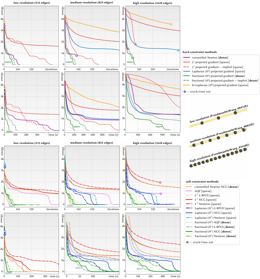
We compared our fractional Sobolev descent strategy to a variety of methods from optimization and geometry processing. Overall, methods that use our fractional preconditioner performed best, especially as problem size increases. We first ran all methods on several resolutions of a small set of test curves (Figure 18); we then took the fastest methods, and ran them on all 228 curves from our two datasets (Figure 19). For simplicity we did not use hierarchical acceleration in our method (and instead just solve dense systems), which gave a significant performance advantage to alternative methods (which are based on sparse solves). Even with this handicap, the fractional approach outperformed all other methods; as indicated in Figure 20, hierarchical acceleration would widen this gap even further. Importantly, previous methods also have a much higher failure rate at untangling difficult curves (Figure 19). Note that some previous methods do not directly handle hard nonlinear constraints; for these methods we perform an apples-to-apples comparison by replacing—in all methods—hard edge length constraints with a soft elastic penalty (see supplemental material for further details).
Knot untangling methods
We first compared to two well-known methods for knot untangling (Figure 15): KnotPlot, based on the so-called symmetric energy, and shrink on no overlaps (SONO) [Pierański 1998] which performs a local iterative projection in the spirit of contemporary position-based dynamics [Müller et al. 2007]. Both methods successfully untangle the Freedman knot, but only after tens of thousands of iterations [Scharein 1998, Figure 7.6]. The basic reason is that, like descent, such methods focus on reduction of local error, making global convergence quite slow.

1st-order methods
Figure 16 indicates that basic 1st-order schemes like ordinary gradient descent, L-BFGS using 10, 30, or 100 vectors, and nonlinear conjugate gradients à la Fletcher and Reeves 1964 exhibit poor performance relative to our fractional scheme in terms of both wall clock time and number of iterations. This example also indicates that for , the next smallest or largest integer Sobolev preconditioners ( and ) underperform the fractional preconditioner, whether using explicit or implicit Euler. Since the implicit update equations are nonlinear, we solved them using Newton’s method—either by updating the Hessian for each Newton step, or “freezing” the Hessian at the beginning of the time step. Here we also tried stochastic gradient descent (SGD) with respect to the inner product, which is currently quite popular in machine learning—this method did far worse than any other scheme we tried. SGD with respect to works better, but the speedup provided by stochastic evaluation does not compensate for the poor quality of the descent direction.

2nd-order methods
Second-order schemes like Newton’s method can be adapted to nonconvex problems by projecting the Hessian onto a nearby positive-semidefinite matrix. Since a global projection is prohibitively expensive, a heuristic sometimes used in geometric optimization is to project and sum up the Hessians of each local energy term [Teran et al. 2005]; in our case we can decompose the energy into the edge-edge terms from Equation 17. Though this heuristic can work well for, e.g., elastic energies, it does not appear to work very well for the tangent-point energy, and for larger examples had among the slowest run times of any scheme we tried (Figure 18).
Quasi-Newton methods
Several recent methods from geometry processing apply Sobolev-like preconditioning to elastic energies, such as those used for shape deformation or surface parameterization [Kovalsky et al. 2016; Claici et al. 2017; Zhu et al. 2018]. Since the highest-order term in such problems often looks like Dirichlet energy, preconditioning via the Laplacian can be an effective starting point for optimization (as discussed in Section 4.1). However, such preconditioners do not perform as well as our fractional preconditioner, since they are not as well-matched to the order of the differential . For instance, as seen in Figure 18, the AQP strategy of Kovalsky et al. 2016 significantly underperforms our preconditioner when the Laplacian is used as the quadratic proxy; using our fractional operator as the quadratic proxy improves performance—but of course requires the machinery introduced in this paper. Another possibility is to use Laplacian-initialized L-BFGS (in the spirit of Zhu et al. 2018); we found this strategy works a bit better than AQP, but again not as well as the fractional preconditioner. We also considered several variants of these strategies, such as applying Nesterov acceleration, and combining nonlinear conjugate gradients (NCG) à la Polak and Ribiere 1969 or L-BFGS with our fractional preconditioner. For hard constraints we advocate the use of our fractional () projected gradient scheme (as detailed in Section 5); if soft constraint enforcement is acceptable, then L-BFGS or -preconditioned NCG are both good options: the former converges faster near minima; the latter gets stuck less often.


7.3. Local minimizers
As seen in Figure 17, the local minimizers found via our fractional descent strategy generally appear to be the same as with other schemes, up to rigid motions. Hundreds more such examples can be found in the supplemental material. Very rarely, two different methods produced local minimizers that were identical up to a reflection; such amphichiral pairs exist in some knot classes [Liang and Mislow 1994], but of course have the same energy.
7.4. Scaling behavior
We compared per-iteration costs of the unaccelerated scheme, a scheme using only Barnes-Hut (Section 6.1), and the full acceleration scheme described in Section 6—see Figure 20. With full acceleration we observe near-linear scaling, whereas schemes that directly solve the dense system exhibit super-quadratic scaling and quickly run out of memory. Note that constraint projection with direct solvers comes nearly for free, since a factorization of Equation 23 can be reused to solve Equation 22. In contrast, no reuse is possible in the fully accelerated scheme, making constraint projection relatively expensive. Disabling this step further speeds up the accelerated scheme, but leads to constraint drift over time. Alternative methods for constraint enforcement (such as soft penalties, as noted above) might hence provide further improvement.

8. Results and Applications
Given how ubiquitous plane and space curves are in areas like geometry, graphics, robotics, and visualization—and how natural it is to want to avoid collision of such curves—our method provides a useful computational framework for a wide variety of tasks. Here we explore some preliminary applications that we hope will inspire future work. All other examples in this section completed within a few minutes, except for the 3D curve packing example where we allowed curves to grow longer for several hours as a stress test. We first describe constraints and potentials used for these examples.
8.1. Constraints and Potentials
A key feature of our optimization framework is that it not only efficiently minimizes knot energies, but that it can do so in conjunction with fairly arbitrary user-defined constraints and penalties (Section 5.3). This opens the door to a rich variety of computational design applications beyond the basic “knot untangling” that has been the focus of previous work. For the applications that will be explored in Section 8, we consider the following constraints:
- •
Barycenter. This fixes the barycenter of the curve to a point via the constraint . In the absence of other constraints, this eliminates the null space of globally constant functions discussed in Appendix A.
- •
Length. The repulsive curve energy naturally wants to make the curve longer and longer. A simple way to counteract this is via a total length constraint , where is the target length.
- •
Edge Length. We can also constrain the lengths of each individual edge, allowing only isometric motions. This entails a constraint for each edge , where is the target edge length.
- •
Point Constraint. To fix the position of a vertex to the point , we can add the constraint .
- •
Surface Constraint. To keep a point of the curve constrained to an implicit surface , we can add the constraint
- •
Tangent Constraint. We can force the tangent of an edge to match a unit vector via the constraint .
In several applications, we progressively increase or decrease the target length values or ; the next constraint projection step then enforces the new length. We also consider the following penalties:
- •
Total length. A simple energy is the total curve length, which provides a “soft” version of the total length constraint. Discretely, this energy is given by .
- •
Length difference. This energy penalizes differences in adjacent edge lengths, given by , where denotes the set of “interior” vertices with degree 2, and and are the indicent edges to .
- •
Surface potential. Given a surface , we use the energy to avoid collisions. This is effectively a Coulomb potential of the same order as on . In the discrete setting, is a triangulated surface, and we use a BVH on to accelerate the evaluation of and its differential, in a similar fashion to .
- •
Field potential. Given a fixed unit vector field on , the energy encourages to run parallel (or anti-parallel) to . We discretize this as .
Note that the energies considered here involve lower-order derivatives than those in , and do not therefore have a major effect on the stiffness of the overall system. Hence, we can continue to use the fractional Sobolev inner product without modification to define an efficient gradient flow.

8.2. Curve Packing
Packing problems (such as bin packing) appear throughout geometry and computer graphics, playing an important role in, e.g., 2D layouts for manufacturing or UV atlas generation. An adjacent problem is generation of regular sampling patterns, e.g., blue noise sampling via Poisson disk rejection. The ability to optimize large families of repulsive curves enables us to solve analogous “curve packing” problems—for instance, in Figure 22, we use a fixed boundary curve to pack disks of increasing length; likewise, in Figures 1 and 23, we use a surface penalty to pack increasingly long curves into a target region. Figure 24 likewise packs increasingly long curves on a surface. Going the opposite direction, we can also decrease length while encouraging repulsion to generate clean illustrations that are difficult to draw by hand (Figure 25). Finally, by constraining only parts of curves to lie on surfaces, we can design biologically-inspired curve networks such as muscle fibers (Figure 21), which are attached to objects at their endpoints but are otherwise free.


8.3. Graph Drawing


A basic problem in data visualization is drawing graphs; a typical approach is to use a force-based layout that seeks to avoid, e.g., collisions between nodes, or over/under-extension of edges [Fruchterman and Reingold 1991]. Our framework makes it easy to optimize the geometry of the edges themselves, opening the door to graph layouts that are both more compact and more legible (Figure 26). We can also use this machinery to obtain legible drawings of nonplanar graphs, by perturbing a planar embedding (Figure 27); here, the ability to preserve lengths conveys information about edge weights. A particularly interesting graph embedding problem is the design of synthetic hydrogel vascular networks [Grigoryan et al. 2019]; Figure 28 shows a simple example where we optimize a multivascular network (starting from subgraphs of a tet mesh and its dual).
![[Uncaptioned image]](2006.07859v1/JunctureConstraint.png)
Note that at junctures between more than two edges, the tangent-point energy will always be large (since three or more edges cannot be collinear), rapidly forcing vertices away from each other. This can be counteracted by constraining their edge lengths, forcing the vertices to lie on spheres of constant radii around the junctures.
8.4. Self-Avoiding Splines
Beyond standard Bézier input, sophisticated tools have been developed for drawing spline curves—but do not consider the basic constraint of ensuring that curves do not cross themselves (which is often desirable for physical or aesthetic reasons). For instance, Figure 30 (center) shows the interpolation of a set of control points by k-curves [Yan et al. 2017], which underpin one of the basic drawing tools in Adobe Illustrator (the Curvature Tool). By simply applying point constraints at the control points, and letting the length increase under our repulsive flow, we obtain a nice interpolating curve without self-intersection (Figure 30, right). In this context we can also use our tangent constraint to control the behavior of such a curve at open endpoints (Figure 29).
8.5. Multi-agent Path Planning

In robotics, numerous algorithms have been developed for the problem of multi-agent path planning [de Wilde et al. 2013], wherein multiple agents must travel from fixed start to end locations without colliding with the environment or each other. Many algorithms operate on a discrete grid or graph [Yu and LaValle 2013], which quantizes the solution space and does not penalize near-collisions; such trajectories may therefore not be robust to sensing or control error. By treating path planning as a space-time optimization of continuous curves with fixed endpoints, we can use curve repulsion to find (or refine) trajectories that maximize collision avoidance, making them more resilient to error (Figure 31). Finding such trajectories in dimensions is equivalent to optimizing a braid in dimensions; since neither the size of the curve nor the cost of a BVH/BCT depends strongly on dimension, this strategy easily generalizes to three (or more) dimensions.
8.6. Streamline Visualization
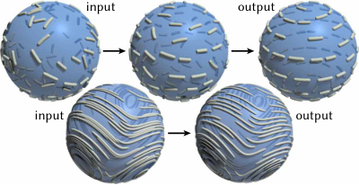
A common way to visualize vector fields is by tracing integral curves or streamlines; significant effort has gone into algorithms that provide uniform spacing (e.g., by incrementally constructing a Delaunay triangulation [Mebarki et al. 2005]), though such methods can be difficult to generalize to 3D volumes or vector fields on surfaces. We can generate nicely-spaced streamlines by adding a field alignment potential to the tangent-point energy—for instance, in Figure 32 we start with a set of random curve segments, which automatically coalesce into streamlines.
9. Limitations and Conclusion
![[Uncaptioned image]](2006.07859v1/StuckCurve.png)
Since we approximate the tangent-point energy via numerical quadrature, it is possible for a very coarse curve to pass through the energy barrier. However, crossings can be prevented via continuous time collision detection (Section 5.4); to maintain accuracy one could also try adding more quadrature points at the previous time step if any collisions occur. For the design tasks in this paper, we did not find such strategies necessary. Also on very coarse meshes, edges that are extremely close together can temporarily get stuck in a near-crossing configuration (see inset). In this situation, the term from the low-order term (Equation 13) is very large, causing the inverse of —and hence the Sobolev gradient—to be very small. One idea is to use adaptive quadrature for edge pairs that are close in space, which would better resolve the near-infinite high-order term and hence push the curve apart. Given the scalability of our approach, another pragmatic solution is simply to increase the overall resolution.
There are many ways to further accelerate our solver. For instance, we did not vectorize our code, parallelized only the matrix-vector multiply in non-well-separated leaves of the BCT, and did not make use of the GPU. For small time steps one might re-fit rather than re-build the BVH; likewise, it may be beneficial to incrementally update the BCT. Better line search or descent direction heuristics may also reduce the overall number of steps.
Finally, a natural question is how to extend these techniques to surface repulsion. The tangent-point energy seems attractive here since (unlike Möbius energy) it needs only Euclidean rather than geodesic distances. One now has double integrals over surfaces, but might still achieve efficiency via hierarchical acceleration. In general, we are hopeful our investigation will provide valuable insight into using repulsive energies for computational design.

Acknowledgements.
Thanks to Stelian Coros for early discussion of these ideas. The bunny mesh is used courtesy of the Stanford Computer Graphics Laboratory. This work was supported by a Packard Fellowship, NSF awards 1717320 and 1943123, and gifts from Autodesk, Adobe, Activision Blizzard, Disney, and Facebook. The second author was supported by a postdoc fellowship of the German Academic Exchange Service and by DFG-Project 282535003: Geometric curvature functionals: energy landscape and discrete methods. The third author was also supported by NSF award DMS-1439786 and Sloan award G-2019-11406 while in residence at ICERM.References
- [1]
- Ainsworth and Glusa [2017] M. Ainsworth and C. Glusa. 2017. Aspects of an Adaptive Finite Element Method for the Fractional Laplacian. Comput. Methods Appl. Mech. Eng. 327 (2017).
- Andrews et al. [2020] B. Andrews, B. Chow, C. Guenther, and M. Langford. 2020. Extrinsic Geometric Flows. Graduate Studies in Mathematics, Vol. 206.
- Angelidis and Neyret [2005] A. Angelidis and F. Neyret. 2005. Simulation of smoke based on vortex filament primitives. In Symp. Comp. Anim. 87–96.
- Ashton and Cantarella [2005] T. Ashton and J. Cantarella. 2005. A fast octree-based algorithm for computing ropelength. In Physical And Numerical Models In Knot Theory. 323–341.
- Ashton et al. [2011] T. Ashton, J. Cantarella, M. Piatek, and E. Rawdon. 2011. Knot tightening by constrained gradient descent. Experimental Mathematics 20, 1 (2011), 57–90.
- Barnes and Hut [1986] J. Barnes and P. Hut. 1986. A hierarchical O(N log N) force-calculation algorithm. Nature 324, 6096 (1986), 446–449.
- Bartels et al. [2018] S. Bartels, P. Reiter, and J. Riege. 2018. A simple scheme for the approximation of self-avoiding inextensible curves. IMA J. Num. Anal. 38, 2 (2018), 543–565.
- Bergou et al. [2008] M. Bergou, M. Wardetzky, S. Robinson, B. Audoly, and E. Grinspun. 2008. Discrete elastic rods. In ACM Trans. Graph., Vol. 27. ACM, 63.
- Blatt [2012] S. Blatt. 2012. Boundedness and Regularizing Effects of O’hara’s Knot Energies. Journal of Knot Theory and Its Ramifications 21, 01 (2012).
- Blatt [2013] S. Blatt. 2013. The Energy Spaces of the Tangent Point Energies. Journal of Topology and Analysis 5, 3 (2013), 261–270.
- Blatt and Reiter [2015] S. Blatt and P. Reiter. 2015. Regularity Theory for Tangent-point Energies: the Non-degenerate Sub-critical Case. Adv. Calc. Var. 8, 2 (2015), 93–116.
- Boyd and Vandenberghe [2004] S. Boyd and L. Vandenberghe. 2004. Convex Optimization. Cambridge University Press.
- Braess and Sarazin [1997] D. Braess and R. Sarazin. 1997. An Efficient Smoother for the Stokes Problem. Applied Numerical Mathematics 23, 1 (1997), 3–19.
- Brakke [1992] K. Brakke. 1992. The surface evolver. Experimental mathematics 1, 2 (1992).
- Brakke [1994] K. Brakke. 1994. Surface evolver manual.
- Brown et al. [2004] J. Brown, J. Latombe, and K. Montgomery. 2004. Real-time Knot-tying Simulation. The Visual Computer 20, 2 (01 May 2004), 165–179.
- Buck and Orloff [1995] G. Buck and J. Orloff. 1995. A simple energy function for knots. Top. Appl. 61, 3 (1995).
- Calvo et al. [2002] J. Calvo, K. Millett, and E. Rawdon. 2002. Physical Knots: Knotting, Linking, and Folding Geometric Objects in . Vol. 304. American Mathematical Society.
- Chern et al. [2016] A. Chern, F. Knöppel, U. Pinkall, P. Schröder, and S. Weißmann. 2016. Schrödinger’s smoke. ACM Trans. Graph. 35, 4 (2016), 77.
- Claici et al. [2017] S. Claici, M. Bessmeltsev, S. Schaefer, and J. Solomon. 2017. Isometry-aware preconditioning for mesh parameterization. In Comp. Graph. Forum, Vol. 36.
- Crane et al. [2013] K. Crane, U. Pinkall, and P. Schröder. 2013. Robust Fairing via Conformal Curvature Flow. ACM Trans. Graph. 32, 4 (2013).
- de Wilde et al. [2013] B. de Wilde, A. ter Mors, and C. Witteveen. 2013. Push and rotate: cooperative multi-agent path planning. In Proc. Conf. Auton. Agents and Multi-agent Sys.
- DeForest and Kankelborg [2007] C. DeForest and C. Kankelborg. 2007. Fluxon Modeling of Low-beta Plasmas. J. Atm. Sol.-Terr. Phys. 69, 1-2 (2007), 116–128.
- Desbrun et al. [1999] M. Desbrun, M. Meyer, P. Schröder, and A. Barr. 1999. Implicit Fairing of Irregular Meshes Using Diffusion and Curvature Flow. In Proc. ACM SIGGRAPH. 8.
- Di Nezza et al. [2012] E. Di Nezza, G. Palatucci, and E. Valdinoci. 2012. Hitchhiker’s guide to the fractional Sobolev spaces. Bull. Sci. Math. 136, 5 (2012), 521–573.
- Eckstein et al. [2007] I. Eckstein, J. Pons, Y. Tong, C. Kuo, and M. Desbrun. 2007. Generalized Surface Flows for Mesh Processing. In Geometry Processing, Alexander Belyaev and Michael Garland (Eds.). The Eurographics Association.
- Ellson et al. [2001] J. Ellson, E. Gansner, L. Koutsofios, S. North, and G. Woodhull. 2001. Graphviz: Open Source Graph Drawing Tools. In Int. Symp. on Graph Drawing. 483–484.
- Fletcher and Reeves [1964] R. Fletcher and C. Reeves. 1964. Function minimization by conjugate gradients. The computer journal 7, 2 (1964), 149–154.
- Freedman et al. [1994] M. Freedman, Z. He, and Z. Wang. 1994. Mobius Energy of Knots and Unknots. Annals of Mathematics 139, 1 (1994), 1–50.
- Fruchterman and Reingold [1991] T. Fruchterman and E. Reingold. 1991. Graph drawing by force-directed placement. Software: Practice and experience 21, 11 (1991), 1129–1164.
- Greengard and Rokhlin [1997] L. Greengard and V. Rokhlin. 1997. A new version of the fast multipole method for the Laplace equation in three dimensions. Acta numerica 6 (1997).
- Grigoryan et al. [2019] B. Grigoryan, S. Paulsen, et al. 2019. Multivascular networks and functional intravascular topologies within biocompatible hydrogels. Science 364, 6439 (2019), 458–464.
- Hackbusch [2015] W. Hackbusch. 2015. Hierarchical matrices: algorithms and analysis. Vol. 49. Springer.
- Harmon et al. [2009] D. Harmon, E. Vouga, B. Smith, R. Tamstorf, and E. Grinspun. 2009. Asynchronous Contact Mechanics. In ACM Trans. Graph., Vol. 28. ACM, 87.
- Hassan et al. [1998] Y. Hassan, S. Easa, and A. Abd El Halim. 1998. State-of-the-art of Three-dimensional Highway Geometric Design. Can. J. Civ. Eng. 25, 3 (1998), 500–511.
- Kleckner et al. [2016] D. Kleckner, L. Kauffman, and W. Irvine. 2016. How Superfluid Vortex Knots Untie. Nature Physics 12, 7 (2016), 650.
- Kovalsky et al. [2016] S. Kovalsky, M. Galun, and Y. Lipman. 2016. Accelerated quadratic proxy for geometric optimization. ACM Trans. Graph. 35, 4 (2016), 1–11.
- Kubiak et al. [2007] B. Kubiak, N. Pietroni, F. Ganovelli, and M. Fratarcangeli. 2007. A Robust Method for Real-time Thread Simulation. In Proc. ACM Symp. Virt. Real. Soft. Tech. ACM, 85–88.
- Kusner and Sullivan [1998] R. Kusner and J. Sullivan. 1998. Möbius-invariant knot energies. Ideal knots 19 (1998).
- Kwaśnicki [2017] M. Kwaśnicki. 2017. Ten equivalent definitions of the fractional Laplace operator. Fract. Calc. Appl. Anal. 20, 1 (2017), 7–51.
- Lackenby [2014] M. Lackenby. 2014. Elementary Knot Theory. Clay Mathematics Institute (2014).
- Ladd and Kavraki [2004] A. Ladd and L. Kavraki. 2004. Motion Planning for Knot Untangling. 7–23.
- Liang and Mislow [1994] C. Liang and K. Mislow. 1994. On amphicheiral knots. J. Math. Chem. 15, 1 (1994).
- Martin et al. [2013] T. Martin, P. Joshi, M. Bergou, and N. Carr. 2013. Efficient Non-linear Optimization via Multi-scale Gradient Filtering. In Comp. Grap. Forum, Vol. 32. 89–100.
- Maucher and Sutcliffe [2016] F. Maucher and P. Sutcliffe. 2016. Untangling knots via reaction-diffusion dynamics of vortex strings. Physical review letters 116, 17 (2016), 178101.
- McCrae and Singh [2009] J. McCrae and K. Singh. 2009. Sketching Piecewise Clothoid Curves. Computers & Graphics 33, 4 (2009), 452–461.
- Mebarki et al. [2005] A. Mebarki, P. Alliez, and O. Devillers. 2005. Farthest point seeding for efficient placement of streamlines. In IEEE Visualization. 479–486.
- Moreton [1992] H. Moreton. 1992. Minimum curvature variation curves, networks, and surfaces for fair free-form shape design. Ph.D. Dissertation. University of California, Berkeley.
- Müller et al. [2007] M. Müller, B. Heidelberger, M. Hennix, and J. Ratcliff. 2007. Position based dynamics. J. Vis. Comm. and Im. Repr. 18, 2 (2007), 109–118.
- O’Hara [1991] J. O’Hara. 1991. Energy of a knot. Topology 30, 2 (1991), 241–247.
- Padilla et al. [2019] M. Padilla, A. Chern, F. Knöppel, U. Pinkall, and P. Schröder. 2019. On bubble rings and ink chandeliers. ACM Trans. Graph. 38, 4 (2019), 129.
- Pérez et al. [2017] J. Pérez, M. Otaduy, and B. Thomaszewski. 2017. Computational design and automated fabrication of kirchhoff-plateau surfaces. ACM Trans. Graph. 36, 4 (2017), 62.
- Pérez et al. [2015] J. Pérez, B. Thomaszewski, et al. 2015. Design and Fabrication of Flexible Rod Meshes. ACM Trans. Graph. 34, 4 (2015).
- Pierański [1998] P. Pierański. 1998. In Search of Ideal Knots. In Ideal Knots, A. Stasiak, V. Katritch, and L. Kauffman (Eds.). Vol. 19. World Scientific.
- Pinkall and Polthier [1993] U. Pinkall and K. Polthier. 1993. Computing discrete minimal surfaces and their conjugates. Experimental mathematics 2, 1 (1993), 15–36.
- Polak and Ribiere [1969] E. Polak and G. Ribiere. 1969. Note sur la convergence de méthodes de directions conjuguées. ESAIM: Math. Model. Num. Anal. 3, R1 (1969), 35–43.
- Redon et al. [2002] S. Redon, A. Kheddar, and S. Coquillart. 2002. Fast continuous collision detection between rigid bodies. In Comp. Graph. Forum, Vol. 21. 279–287.
- Renka and Neuberger [1995] R. Renka and J. Neuberger. 1995. Minimal Surfaces and Sobolev Gradients. SIAM Journal on Scientific Computing 16, 6 (1995), 1412–1427.
- Scharein [1998] R. Scharein. 1998. Interactive Topological Drawing. Ph.D. Dissertation. University of British Columbia.
- Schumacher [2017] H. Schumacher. 2017. On -gradient Flows for the Willmore Energy. arXiv e-prints (Mar 2017).
- Smith and Schaefer [2015] J. Smith and S. Schaefer. 2015. Bijective parameterization with free boundaries. ACM Trans. Graph. 34, 4 (2015), 1–9.
- Strzelecki and von der Mosel [2017] P. Strzelecki and H. von der Mosel. 2017. Geometric curvature energies: facts, trends, and open problems. In New Directions in Geometric and Applied Knot Theory.
- Teran et al. [2005] J. Teran, E. Sifakis, G. Irving, and R. Fedkiw. 2005. Robust quasistatic finite elements and flesh simulation. In Symp. Comp. Anim. 181–190.
- Triebel [1983] H. Triebel. 1983. Theory of function spaces. Monographs in Mathematics, Vol. 78.
- Walker [2016] S. Walker. 2016. Shape optimization of self-avoiding curves. J. Comp. Phys. 311 (2016).
- Weißmann and Pinkall [2010] S. Weißmann and U. Pinkall. 2010. Filament-based smoke with vortex shedding and variational reconnection. In ACM Trans. Graph., Vol. 29.
- Yan et al. [2017] Z. Yan, S. Schiller, G. Wilensky, N. Carr, and S. Schaefer. 2017. k-curves: interpolation at local maximum curvature. ACM Trans. Graph. 36, 4 (2017).
- Yu et al. [2017] C. Yu, K. Crane, and S. Coros. 2017. Computational Design of Telescoping Structures. ACM Trans. Graph. 36, 4 (2017).
- Yu and LaValle [2013] J. Yu and S. LaValle. 2013. Multi-agent path planning and network flow. In Algorithmic Foundations of Robotics X. Springer, 157–173.
- Zehnder et al. [2016] J. Zehnder, S. Coros, and B. Thomaszewski. 2016. Designing structurally-sound ornamental curve networks. ACM Trans. Graph. 35, 4 (2016), 99.
- Zhu et al. [2018] Y. Zhu, R. Bridson, and D. Kaufman. 2018. Blended cured quasi-newton for distortion optimization. ACM Trans. Graph. 37, 4 (2018), 1–14.
Appendix A Sobolev-Slobodeckij Gradient
How do we obtain an ideal gradient flow for the tangent-point energy (i.e., one that behaves like an ODE)? Unlike standard energies (elastic energy, Willmore energy, etc.), an answer to this question has not yet been worked out formally. However, we can make an educated guess based on past wisdom about curve energies.
In general, suppose an energy has a (Fréchet) differential . To determine the highest-order derivatives, it is not necessary to derive an explicit expression for as we did for the Dirichlet energy (Section 4.1). Instead, we can reason about the associated function spaces: as long as we know the order of , we can “cancel” spatial derivatives by constructing an inner product of the same order.
For the tangent-point energy, existing analysis gives the maximum order of derivatives in (Appendix A.2), from which we deduce the order of (Appendix A.3). What is unusual here is that the number of derivatives is fractional (Appendix A.1.2); to build an inner product of appropriate order, we therefore start with the fractional Laplacian (Section A.1), and formulate an analogous operator for embedded curves. Taking further (integer) derivatives then yields an operator of the same order as (Appendix A.4). From there, we use additional heuristics (inspired by numerical experiments) to choose a low-order term that makes this operator well-behaved and invertible (Appendix A.4.2), allowing us to use it in the definition of a fractional Sobolev gradient (Section 4.2).
A.1. Fractional Analysis
We begin with a brief discussion of Sobolev spaces of fractional order ; for further background, see [Di Nezza et al. 2012].
A.1.1. Fractional Differential Operators
Whereas standard differential operators are purely local (i.e., the value of depends only on an arbitrarily small neighborhood of ), fractional differential operators are nonlocal ( can depend on the value of at any point ). Since the tangent-point energy is nonlocal, it will also have nonlocal derivatives. Hence, finding an inner product well-matched to its gradient flow entails constructing an appropriate fractional differential operator—an important example in our setting is the fractional Laplacian on , which is commonly defined by taking powers of the eigenvalues in the spectral expansion. For and all sufficiently regular , the operator can also be expressed via the integral
| (24) |
where the constant depends only on and [Kwaśnicki 2017]. The behavior of this operator is illustrated in Figure 34.
A.1.2. Fractional Sobolev Spaces
There are two common ways to understand Sobolev spaces of fractional order. One is to consider the Fourier transform of the Laplacian , leading to the Bessel potential spaces [Triebel 1983, Section 2.2.2]. For us, however, this viewpoint helps only to understand the case . The other, essential for studying the tangent-point energy, is via the Sobolev-Slobodeckij spaces . Functions in these spaces look like functions in an ordinary Sobolev space, but with a nonlocal regularity condition on the highest-order derivative . In particular, suppose we write for and . Then, on an -dimensional Riemannian manifold , one defines
The expression in square brackets is the (Gagliardo) semi-norm
where is the shortest distance between and in . Just as a Lipschitz function is more regular than an arbitrary continuous function without being differentiable, a function in is more regular than one in , without getting a whole additional derivative (i.e., ). Figure 35 shows an example.

Dual Space.
Just as the dual of the classical Sobolev space is (where ), the dual of the Sobolev-Solobdeckij space can be characterized as a space with “ derivatives” in the sense that the fractional Laplacian identifies with [Di Nezza et al. 2012, Remark 2.5].
A.2. Energy Space
To determine the order of the tangent-point differential , we first consider the biggest space of functions for which the energy is well-defined. Blatt 2013 gives the following condition on the differentiability of the curve (see also Blatt and Reiter 2015):
Lemma A.1.
Suppose and , let , and consider an embedded curve . Then has finite tangent point energy if and only if, up to reparameterization, .
In other words, the tangent point energy is well-defined only for curves that have an th derivative, and for which the th power of that derivative is integrable—for example, it will not be finite for a polygonal curve. The somewhat unusual situation is that is not an integer: instead, it is a fractional value in the interval .
A.3. Order of the Differential
In general, if an energy is defined for functions in a space , then its differential will have the prototype , where is the dual space. For instance, the Dirichlet energy operates only on functions . Hence, its differential is a map , which we saw explicitly in Section 4.1: given a function , produces a linear map from functions in to real numbers, i.e., an element of .
In the case of the tangent point energy, then, we get that is a map from to the dual space (Section A.1.1). Hence, is a “differential operator” of order , i.e., it reduces the differentiability of its argument by . To get a well-behaved flow, we should therefore pick an inner product of the same order, and (for computational purposes) is reasonably easy to invert.
A.4. Fractional Inner Product
Just as one uses the Laplace operator to define integer Sobolev inner products, we use a fractional operator to define a fractional Sobolev inner product. For an embedded curve , one idea is to start with the 1D fractional Laplacian . Alternatively, we can define an analogous operator by replacing the intrinsic distance on the right-hand side of Equation 24 with the extrinsic distance between points in the embedding. This latter construction yields an operator defined by the relationship
| (25) |
for all sufficiently regular . For any , both and are fractional operators of order . But the benefit of is that it requires only Euclidean distances—which for embedded curves are easier to evaluate than geodesic distances. Moreover, building a fractional Laplacian via an explicit Fourier transform is prohibitively expensive, requiring a full eigendecomposition of a discrete Laplace matrix. In contrast, integral expressions like Equations 24 and 25 can easily be evaluated à la Section 5.2.3, and accelerated using hierarchical techniques à la Section 6.
A.4.1. High-Order Term
To get an inner product of the same order as , we compose the operator with further (integer) derivatives . In particular, Lemma A.1 implies that for . Hence, to define an operator of order , we apply two additional derivatives to , i.e., we say that
for all sufficiently regular . This relationship provides the definition of in Equation 12.
A.4.2. Low-Order Term
As discussed in Section 4.2.2, the operator is not invertible. We hence add the low-order term from Equation 13. Since and exhibit the same scaling behavior under a rescaling of , the behavior of the resulting gradient flow will not depend on the global scale. To see why, consider a rescaling of the curve by a factor . Then scales by a factor , the term scales by , and the measure scales by . Then scales by and scales by just . Hence, to get we multiply by , which scales like (since it has in the numerator, and in the denominator). More generally, one could use for any such that . This low-order term also tends to accelerate the evolution of the flow by preserving near-constant motions that slide near-tangentially and do not tend toward collision (Figure 7).
Appendix B Acceleration Scheme
B.1. Energy and Differential Evaluation
B.1.1. Bounding Volume Hierarchy
To build the BVH we first construct tangent-points for each edge . We then cycle through all six coordinates, choosing a splitting plane that minimizes the sum of squared diameters of the two child bounding boxes. Below a user-specified threshold, all remaining tangent-points are placed in a single leaf node. In each node we also store data needed for Barnes-Hut. Specifically,
give the total mass, center of mass, and (length-weighted) average tangent, resp.; we will use to denote the corresponding tangent-point. We also store the bounding box radii and with respect to spatial and tangential coordinates, resp.
B.1.2. Barnes-Hut Approximation
To evaluate the energy for a tangent-point with mass , we traverse the BVH from the root, checking at each node if a local approximation is admissable (see below). If so, we evaluate the approximation
| (26) |
and terminate traversal; otherwise, we sum the energy of the two children. If we reach a leaf node , we directly add up the contributions of the edges contained in this node, i.e.,
Admissibility
A simple Taylor series analysis of Equation 26 indicates that to keep approximation error below a user-specified threshold , it is sufficient to ensure that
| (27) |
Intuitively, if is far from the query point relative to its size, and contains tangents that are close together, then the “lumped” energy is a good approximation of the total energy between edge and the edges in .
Differential
Rather than differentiate our Barnes-Hut approximation of , we approximate the differential of the (full) discrete energy directly. Starting with the zero vector , we perform a BVH traversal for the tangent point associated with each edge . At each admissible node and for each endpoint , of we increment the differential via
Here, is the discrete kernel defined in Equation 18; note that , , and do not depend on or , since is not contained in any admissible node . At any leaf node we add the corresponding derivatives for all edges .
B.2. Hierarchical Matrix-Vector Product
B.2.1. Block Cluster Tree (BCT)
A BCT partitions a matrix into low-rank blocks that approximate the original entries (Figure 12). It is like a quadtree, except that the matrix ordering is not fixed a priori. The basic idea is that the edges in a BVH node correspond to a subset of BCT rows/columns. A block of the BCT is hence specified by a pair of nodes from the BVH. To construct a BCT, we recursively split the root block , where is the root of the BVH. A block is a leaf if and only if (i) it is well-separated, i.e., it provides a good approximation of the local double sum, or (ii) or contains just a few edges. Otherwise, this block is given four children , , , , where are the children of in the BVH (and likewise for ). The conditions for being well-separated are similar to Equation 27:
| (28) |
where and are the spatial and tangential radii of node .
B.2.2. Matrix-Vector Product
The BCT is used to accelerate a matrix-vector product via the fast multipole method. We adopt the lowest (0th) order version of this method, which is accurate enough for preconditioning. In particular, for any admissible leaf node , the midpoints and tangents of edges in and are quite coherent relative to the distance between them. Since the kernel is regular, the restriction of to rows and columns is hence well-approximated by
where is the vector of edge lengths in . Using this rank-1 approximation, matrix-vector multiplication amounts to a single dot product (with ), followed by a scalar-vector product.
To perform a multiplication, we start with the zero vector and iterate over all BCT leaves. For each admissible leaf (i.e., one which satisfies Equation 28) we perform an update
For inadmissible leaves, we simply sum over all edge pairs:
for all . To accelerate evaluation, we percolate these sums up and down the BVH, following a standard fast multipole strategy.
B.3. Multigrid Solver
We first sketch out a generic multigrid strategy for saddle-point problems on a curve network; the specific solves needed for the tangent-point energy are detailed in Appendix B.3.4.
B.3.1. Geometric Multigrid
Suppose we want to solve a linear equation . The basic idea of geometric multigrid is to use a coarser mesh to reduce the residual of an equation on the finer mesh. Consider a simple two-level hierarchy—in particular, let and be discretizations of on a fine and coarse mesh, resp., and let be a discretization of the function onto the finest mesh. Also let be a so-called prolongation operator, which interpolates data from the coarse mesh onto the fine mesh. Starting with any initial guess , we first apply a smoothing procedure to the system , i.e., a fixed number of iterations of any iterative linear solver to get an improved guess . We then compute the residual , and transfer it to the coarse mesh via . On the coarse mesh we solve the system directly, and transfer the result back to the fine mesh via . These values are used to update our guess via , and smoothed again. If the residual is small enough, we stop; otherwise, we repeat another such V-cycle until convergence. More generally, one can apply this two-level strategy to solve the linear system on the coarser level, yielding a multi-level strategy. The size of the coarsest level is chosen so that a direct solve at this level is more efficient than continuing to apply multigrid.
Initialization.
We get an initial guess by first coarsening the fine right-hand side down to the coarsest mesh. We then perform a direct solve and prolong the solution all the way to the finest mesh, applying smoothing after each refinement. In practice this strategy works much better than starting with the zero vector.
Implementation Details
In practice we use a standard conjugate gradient smoother, and typically need 6 or fewer V-cycles to achieve a relative residual of order . Making the residual smaller via further cycles (and a more accurate BCT) yields diminishing returns: we need only a reasonable intermediate descent direction. Note that although we build a BCT at each level, overall construction cost is only about twice the cost at the finest level.
B.3.2. Curve Coarsening and Prolongation
To build a multigrid hierarchy on a general curve network, we apply a simple coarsening scheme. We mark alternating vertices as “black” and “white”, and mark all endpoints and junctures where two or more curves meet as black. The next coarsest curve is obtained by removing white vertices, and we stop when we reach a target size or when there are no more white nodes. The prolongation operator preserves values at black vertices, and at white vertices takes the average of the two neighboring black vertices. In our experience, using linear interpolation based on edge lengths made no appreciable difference in multigrid performance. Although coarsening can change the isotopy class of the curve network, it still provides useful preconditioning for the next level of the hierarchy.
B.3.3. Multigrid for Saddle Point Problems
Our constraint scheme entails solving saddle point problems of the form
| (29) |
where is the inner product (for vector-valued functions) (see Equation 19), and is the constraint matrix (Section 5.3.1); the data depends on the problem being solved. We follow the approach of Braess and Sarazin 1997, who note that for the structurally identical Stokes’ problem (where and are replaced by the Laplace and divergence operators, resp.), applying multigrid to the whole matrix does not work well. Instead, let be a projection onto the null space of , i.e., and . Then by construction, any solution to the equation
| (30) |
yields a vector within the constraint space that satisfies our original equation. Equation 30 is therefore the system that we actually solve via multigrid. In particular, we use the projection , where denotes the (Moore-Penrose) pseudoinverse
Since our constraints are typically sparse, we can factorize the inner term (once per time step) to further accelerate computation. Note that one must build a constraint matrix and projection matrix at each level of the multigrid hierarchy.
B.3.4. Gradient Solve and Constraint Projection
With these pieces in place, we can apply multigrid to compute the constrained gradient (Equation 22), and perform constraint projection (Equation 23).
Gradient
To compute the gradient, recall that . A matrix-vector product can be expressed as
| (31) |
where is a diagonal matrix with entries , averages values from vertices to edges (i.e., ), and
| (32) |
We use the method from Appendix B.2 to efficiently perform the products and , and ordinary sparse matrix multiplication for . The high-order part is expressed exactly as in Equation 31, except that (i) we replace the averaging operator with the difference operator , (ii) we define a different kernel matrix by replacing with in Equation 32, and (iii) just like , acts blockwise on the three components of vector-valued data (à la Equation 19).