A Generalized Asymmetric Dual-front Model for Active Contours and Image Segmentation
Abstract
The Voronoi diagram-based dual-front scheme is known as a powerful and efficient technique for addressing the image segmentation and domain partitioning problems. In the basic formulation of existing dual-front approaches, the evolving contour can be considered as the interfaces of adjacent Voronoi regions. Among these dual-front models, a crucial ingredient is regarded as the geodesic metrics by which the geodesic distances and the corresponding Voronoi diagram can be estimated. In this paper, we introduce a new dual-front model based on asymmetric quadratic metrics. These metrics considered are built by the integration of the image features and a vector field derived from the evolving contour. The use of the asymmetry enhancement can reduce the risk for the segmentation contours being stuck at false positions, especially when the initial curves are far away from the target boundaries or the images have complicated intensity distributions. Moreover, the proposed dual-front model can be applied for image segmentation in conjunction with various region-based homogeneity terms. The numerical experiments on both synthetic and real images show that the proposed dual-front model indeed achieves encouraging results.
Index Terms:
Eikonal equation, asymmetric quadratic metric, Voronoi diagram, active contours, image segmentation, fast marching m ethod.I Introduction
Active contour models have been dedicated to suitably address many image segmentation tasks in a wide variety of computer vision and image analysis scenarios in the past three decades. Basically, image segmentation tasks carried out by an active contour model is usually implemented via a curve evolution scheme. In essence, this scheme can be governed by the contour representation methods in conjunction with the image data-based energy functionals.
Since the original work of the snakes model [1], great efforts have contributed to investigate suitable energy functionals to satisfy a wide variety of image segmentation situations. In other words, the associated active contour approaches attempt to find proper ways on how to utilize the image features to define the objective boundaries. The edge-based features such as the image gradients are widely utilized by many active contour approaches. Interesting examples for edge-based active contour approaches may include the geometric models [2, 3, 4, 5], the external force-based models [6, 7, 8, 9] and the models relying on minimal cost paths [10, 11, 12]. In [13, 14], the edge anisotropy features are taken into account , leading to more general geometric active contours models. The use of edge features removes the effects from image gray level or color homogeneities, yielding practical applications. However, the contour evolution driven by edge-based features may be trapped into unexpected local minima due to the presence of spurious edges probably generated by noises.
The region-based active contour models usually derive the gradient flows by minimizing energy functionals involving region-based homogeneity terms. The Mumford-Shah functional [15] invokes a piecewise smooth fitting function to approximate the image data. The approximation is carried via a region-based term that characterizes the errors between the image gray levels and the the data fitting function. Following the Mumford-Shah piecewise smooth functional, a series of region-based active contour models were introduced to address various image segmentation issues. These models either consider the suitable variants of the Mumford-Shah functional [16, 17, 18, 19] or introduce practical avenues to search for the solutions [20, 21, 22, 23, 24]. The histograms or probability density functions of the image features such as image colors, gray levels and gradients as reviewed in [25], are often used to build nonparametric energy functionals, which can avoid to assume prior distribution of image intensities as introduced in the literature [26, 27]. Recently, a new type of region-based active contour models based on the pairwise similarity-based energy functionals were introduced in [28, 29], which have obtained encouraging results. The active contour models mentioned above are obviously not exhaustive, interesting and effective approaches may include [30, 31, 32, 33, 34, 35].
Contour Representation. The representation for evolving contour is a fundamental and challenging problem in active contour approaches. The parametrized contour method has been used in many approaches [1, 6, 8], due to its low computation complexity. However, this method often suffers from the self-crossing during the contour evolution. In order to obtain expected results, additional procedures are often required to alleviate that issue [36].
The level set scheme [37] has been broadly exploited to search for suitable solutions to active contour evolution [3, 5, 4] due to its solid mathematical background and the rich numerical implementation methods [38, 39, 40, 41]. By the level set framework, the contour evolution can be regarded as a way of updating a Lipchitz function , where is an open and bounded domain of dimension . In its basic formulation, the boundary of a region can be implicitly represented as the zero-level set of such that . In this case, a point is inside if and outside for . The variational level set method [38, 17] made use of the Heaviside function in conjunction with to assign a label to each point , where implies that . Nevertheless, acts as the characteristic function of the region . However, minimizing an energy functional with respect to a level set function (LSF) corresponds to a local minimum, thus increasing the risk of finding unexpected image segmentation. Moreover, a small time step is usually adopted in order to find stable numerical solutions to the level set evolution equations, which will increase computation cost.
The convex relaxation minimization framework [42, 43, 44] was introduced to address the above issues of the level set method in some extent. The convex relaxation schemes are able to find the global minimum of an active contour energy. Specifically, the active contour energy functionals, which are usually comprised of a region-based term and a regularization term, are reformulated by replacing the binary-valued characteristic function using a function . As a consequence, the segmented regions can be derived by thresholding the solutions . The convex relaxation framework has been proven to achieve lower computation complexity than that of the level set scheme and has been successfully applied in many segmentation tasks [22, 45].
Image segmentation approaches based on the concept of Voronoi diagram have obtained promising segmentation results in various segmentation tasks. Among them, the Voronoi diagram can be constructed from several user-provided scribbles respectively placed in the foreground and background regions, as introduced in [46, 47, 48]. Therefore, the user intervention can be naturally incorporated into the segmentation procedure. Alternatively, the Voronoi diagram can be investigated for active contour evolution, for which the basic idea is to represent a contour segment as the interface of two adjacent Voronoi regions. Along this research line, Voronoi regions can be generated through the offset lines of the evolving contour using either geodesic distances [49] or with Euclidean distances [41, 50]. Specifically, the Voronoi implicit interface (VII) scheme [41] is a variant of the original level set method [37], where the LSF is set as a non-negative Euclidean distance map associated to the evolving contour. In the context of multiphase segmentation, unlike the traditional level set method or the convex relaxation method, which require multiple or to characterize all regions, only one single LSF is sufficient for the VII scheme-based dual-front model [50] to represent all disjoint regions. However, the VII model still needs to address the classical level set evolution problem in order to evolve the offset lines of the current contour, which may suffer from the issues of, for examples, high computation cost and sensitivity to the parameters. Li and Yezzi introduced a dual-front model [49] which exploited geodesic distance maps derived from minimal weighted curve length to generate Voronoi regions and to reconstruct the respective Voronoi interface. The region-based homogeneity features and the edge appearance features can be simultaneously encoded into Voronoi diagram construction. The main advantages of this model lie at the efficiency of the numerical solutions and at the flexibility in the extension to multi-region segmentation applications. However, the isotropy limitation of the metrics used in this classical model may suffer from the shortcut problem, i.e. the contour evolution stabilizes before reaching the true boundaries, especially when the object regions have complicate intensity distributions.
Contributions and Paper Outline. In this paper, we propose a new Voronoi diagram-based contour evolution model based on a Finsler metric with an asymmetric quadratic form, which is capable of integrating asymmetry enhancement as well as the image features for Voronoi diagram construction. The main contributions are twofold:
- •
Firstly, we generalize Li and Yezzi’s isotropic dual-front model [49] to an asymmetry-enhanced case. Instead of using direction-independent metrics, the proposed model encapsulates a type of Finsler geodesic metric with an asymmetric quadratic form. The asymmetry property of the considered metric serves as an efficient constraint for front propagation, so as to reduce the risk of the shortcut issue in Voronoi diagram-based segmentation applications.
- •
Secondly, we propose a new method for the construction of data-driven asymmetric quadratic metrics. The ingredients of these metrics are respectively derived from the anisotropic image edge-based features such as image gradients, a variety of region-based homogeneity terms, and the predicted motion directions of the contour. As a result, the image segmentation via the proposed dual-front model can blend the benefits from these features.
The structure of this manuscript is organized as follows. In Section. II, we introduce the preliminaries on the construction of the Voronoi diagram and the corresponding applications for dual-front models. Sections III and IV present the main contribution of this paper: the construction of data-driven asymmetric quadratic metrics for Voronoi diagram-based image segmentation. The experimental results on both synthetic and real images are given in Section V and the conclusion is presented in Section VI. The current document is an extension of the short conference paper presented in [48], upon which more contributions were added.
II Voronoi Diagram-based Contour Evolution
II-A Preliminaries on Voronoi Diagram
The Voronoi diagram is known as a powerful geometric tool for domain partitioning and image segmentation [51, 52, 53, 54]. The construction of Voronoi diagram, regarded as a tessellation of the domain , can be naturally and efficiently implemented through geodesic distance maps. Each geodesic distance map, denoted by and indexed by , is constructed from a set of source points. The distance value at any point represents the weighted length of the minimal path between the source point set and , measured by a local metric . At any fixed point , a metric can be defined using an asymmetric norm on such that for any vector .
Let us denote by the set of Lipschitz continuous curves subject to and . Once the geodesic metric and the source point set are given, a crucial ingredient for estimating a geodesic distance map lies at the definition of the minimal weighted length
| (1) |
where is the first-order derivative of curve . Then the geodesic distance map associated to the set reads
| (2) |
As in [55, 56, 57], the geodesic distance map is a viscosity solution to the Eikonal equation
| (3) |
where is the standard Euclidean gradient of over the domain , and is a Hamiltonian
| (4) |
From the geodesic distance maps for , one can generate Voronoi regions, denoted by , each of which is defined as follows
| (5) |
In this case, a point implies that is precisely closer to than to any other () in the sense of geodesic distance. We say that two distinct Voronoi regions and are adjacent if the set of points which are equidistant to and is not empty.
Voronoi diagram associated to multiple metrics. We have presented the basic procedure for the construction of Voronoi diagram based on the geodesic distance maps. One can see that all the geodesic distance maps are derived using the same metric . In our Voronoi diagram-based contour evolution model (also in [49]), we allow each geodesic distance map to be computed using different metrics
| (6) |
In other words, each geodesic distance map is estimated by an individual metric .
II-B Voronoi Diagram for Dual-front Models
In this section, we briefly summarize the Voronoi diagram-based dual-front models, by which the image segmentation problems can be naturally addressed in an iterative manner. Significant examples include the model based on the VII scheme [50] and the model based on geodesic distance [49]. In each iteration, both dual-front models can be loosely divided into three steps: extracting the offset lines of the evolving contour, building the Voronoi diagram and reconstructing the new contour. The generic algorithm for the Voronoi diagram-based dual-front models are presented in Algorithm 1.
Let be a finite set of curves, which is referred to as a contour in the following. During the contour evolution, can be taken as the input of both dual-front models for 2D image segmentation11 1 In this paper, we focus on the 2D image segmentation and the extension to 3D volume segmentation is straightforward., i.e. the dimension . In general, the input partitions the image domain into open and bounded connected regions for such that and . Let be the interface between two adjacent regions and . We consider a collection of subregions
| (7) |
where denotes the unsigned Euclidean distance between a point and a set , i.e.
| (8) |
II-B1 The VII scheme-based dual-front model
In the VII scheme-based dual-front model [50], the offset lines are extracted from an evolved LSF . The evolution of is driven by minimizing an energy functional comprised of an image data term and a regularization term. Significant examples considered in [50] involve the region competition model [16] and the pairwise similarity models [28, 58], of which the image data-driven terms can be summarized as
| (9) |
where . The motion equation with respect to a time parameter for minimizing can be formulated for any point as follows
| (10) |
where stands for the inward unit normal to the boundary at , and is a set involving all indices such that . The velocity functions for are defined being such that
| (11) |
As discussed in [50], these velocity functions should be extended to the image domain or to a narrow band neighbourhood of , in order to drive the update scheme for the LSF . In the following, we denote by the respective extension of for , subject to .
The VII method initializes the evolving LSF as with being the unsigned Euclidean distance map associated to , see Eq. (8). Using the extended velocity functions , one can define a new velocity function formulated as follows [50]
| (12) |
Accordingly, the LSF evolution equation associated to Eq. (10) reads as
| (13) |
At some time , each evolved offset line, noted as , is the -level set of the solution to the evolution equation (13). For a small , one has
Once all the offset lines are extracted, the construction of the Voronoi diagram in a narrow band can be implemented using the method presented in Section II-A, by setting and .
II-B2 The geodesic distance-based dual-front model
Li and Yezzi [49] proposed a dual-front model, where the construction of the Voronoi diagram is implemented by geodesic distances associated to a family of data-driven isotropic metrics. In the basic setting of the Li-Yezzi model, the offset lines of the boundaries () can be simply extracted by leveraging the -level set of
| (14) |
The second step in the Li-Yezzi model is to reconstruct the Voronoi regions within a neighbourhood of
| (15) |
via a family of geodesic distance maps , as in Section II-A. Each geodesic distance map exploits the offset line as the set of source points, and can be estimated by solving the Eikonal PDE (3). In the Li-Yezzi model, the distance maps are estimated using isotropic Riemannian metrics. These metrics integrate both the magnitude of image gradients and the mean and variance of the image intensities in each region . As an important shortcoming, the isotropic metrics invoked in the Li-Yezzi dual-front model are independent to the expected motion directions of the contour, which may increase the possibility of the evolving contour to suffer from the shortcut problem. In this paper, we propose a new dual-front model to overcome this drawback, by extending the isotropic metrics to the asymmetric quadratic metrics.
III Voronoi Diagram for Dual-front Model from Asymmetric Quadratic Metrics
In this section, we present our core contribution on the construction of the asymmetric geodesic metrics depending on the image data such as the region-based homogeneity terms and image gradients. We first introduce the general form of these metrics considered and then present the principle for their construction in the context of contour evolution.
III-A Asymmetric Quadratic Metrics
Let be a set of symmetric positive definite matrices of size . In this section, we consider an asymmetric quadratic metric which is made up of a tensor field and a vector field
| (16) |
where stands for the Euclidean scalar product on . The second term in Eq. (16) involves a scalar product which can be expressed as [59]
| (17) |
and .
The asymmetric quadratic metric in Eq. (17) should be positive, -homogeneous and convex w.r.t its second argument. The positivity and homogeneity properties are clearly satisfied. The proof for the convexity property of the asymmetric quadratic metric is presented in Proposition 1 of Appendix -A. Moreover, the metric formulated in Eq. (16) is asymmetric with respect to its second argument due to the existence of the second term (17). Note that when the vector field , the metric gets to a symmetric Riemannian metric, i.e. .
It is a popular way to utilize the tool of control sets for the visualization of a geodesic metric. The control set for any point is defined as the unit ball of the metric
| (18) |
The unit ball is governed by both of the matrix and the vector . In Fig. 1, we illustrate the unit balls with respect to different matrices and vectors . In Fig. 1a, we set where is an identity of size , and . The corresponding unit ball appears to be a disk, since gets to be isotropic in this case. Furthermore, assuming that and keeping , the vector leads to a unit ball close to a half disk, as depicted in Fig. 1b. The metric has high values if the vectors . Finally, we use and , where is the vector orthogonal to . In this case, the control set approximates a half ellipse, as shown in Fig. 1c. In Fig. 2, we illustrate the geodesic distance maps and the corresponding Voronoi regions. In each column of this figure, the distance map is estimated using a metric at any point satisfying the control set shown in the respective column of Fig. 1.


III-B Constructing Data-driven Asymmetric Quadratic Metrics
III-B1 Data-driven Asymmetric Quadratic Metrics
We denote by a given contour, which partitions the image domain into open and bounded regions and yields offset lines by means of Eq. (14). In order to reconstruct the Voronoi regions , we consider the following image data-driven asymmetric quadratic metrics
| (19) |
where is a positive scalar-valued function. The tensor field carries out the edge anisotropy and appearance features derived from the image gradients. The scalar-valued functions and the vector fields with are dependent to the region-based homogeneity terms considered. The computation for these ingredients of the data-driven asymmetric quadratic metrics (19) will be described in the following.
In the proposed dual-front model, in order to reduce the computation costs, the estimation for each geodesic distance map is restricted in a tubular neighbourhood of the boundary , where is the neighbourhood of the whole contour , see Eq. (15). Such a neighbourhood , abbreviated as , can be expressed as
| (20) |
Furthermore, we also apply that restriction to the construction of the asymmetric quadratic metrics (19). In other words, each data-driven metric is defined over the domain .
III-B2 Principle for constructing data-driven metrics
Given a suitable constant , one can extract the -level set lines from the Euclidean distance map . In the VII scheme-based active contour model [50], the LSF evolution equation (13) also characterizes the evolution of the level set lines for , leading to a fact that a point will move along the direction , where is the velocity function defined in Eq. (12). In this case, we introduce a family of vector fields indexed by as follows
| (21) |
and otherwise, where is the sign of a scalar value . Recall that is the inward normal vector to the boundary at . The vectors indicate the motion directions of the level set for , which point to the desired boundary from . Nevertheless, we consider to exploit these vector fields to construct the vector fields for .
From the viewpoint of front propagation, a front is a level set line of the geodesic distance map emanating from the offset line . At some point , the advancing direction, denoted by , of the front subject to is positively proportional to . Therefore, we encourage that the front , which passes through the point , propagates fast in case its advancing direction forms an acute angle with , i.e. . Towards this purpose, we construct the vector fields for as
| (22) |
where is a constant as a weighted parameter.
In addition, the function can be estimated for any point as follows
| (23) |
where is a constant and is the Voronoi region associated to as defined in Eq. (7).
Remark. Note that the vector fields (or ) dominate the front propagation speed especially within the homogeneous regions where the image gradients are small. As a consequence, the use of asymmetric quadratic metrics (19) allows us to perform the front propagation independently to the weighted functions . Therefore, in contrast to the classical isotropic dual-front model [49], the introduced dual-front evolution scheme featuring asymmetric property could in principle be implemented using one single metric with for such that for any point , and . This potential simplification was one of our initial motivations for the study of Voronoi diagram-based active contours associated to asymmetric metrics. However, in the end, we found that the best efficiency can be achieved by combining the advantages of both (i) asymmetric geodesic metrics, and (ii) distinct weighted functions for the propagation of the respective fronts.
III-C Edge Anisotropy Features from Image Gradients
The construction of the tensor field relies on the image gradients, which carries out the edge anisotropy information. With respect to a vector-valued image in the RGB color space, we apply the method introduced in [60, 61] to estimate the image gradients for a Gaussian-smoothed image. Let be a Gaussian kernel with a standard deviation and we denote by the Euclidean gradient of . At each point , we first compute a Jacobian matrix of size
| (24) |
where and ‘’ is a convolution operator. Furthermore, for a gray level image , the equation (24) gets to be . When smoothing the images via , high values of can suppress the effects from noise, but may potentially increase the risk of missing weak edges.
The eigenvectors of the matrix , referred to as for , can be used to characterize the edge anisotropy features. Among them, the eigenvector which corresponds to the largest eigenvalue of can be used to indicate the direction perpendicular to the edge tangent at .
The edge appearance features are carried by a scalar-valued function defined by
| (25) |
where is the Frobenius norm of the matrix
By means of the eigenvectors , and the normalized Frobenius norms , we construct the tensor field as follows
| (26) |
and otherwise, where is the identity of size and where reads
| (27) | ||||
| (28) |
where are two constants. Specifically, the values of dominate the anisotropy property of , while controls the relative importance on the edge appearance features.
Eventually, we smooth the tensor field via a Gaussian kernel with standard deviation
| (29) |
Each entry of the matrix is generated by convolving the corresponding entry of via . The value of the standard deviation is fixed in the following experiments.


IV Implementation Consideration
IV-A Smooth the Vector Fields
The vector fields dominate the front propagation. In this section, we smooth by means of a Gaussian kernel in order to alleviate the effects from discretization. For this purpose, we first consider the following matrix field
| (30) |
where is a Gaussian kernel with standard deviation .
Let us denote by the eigenvector of the matrix which corresponds to the largest eigenvalue of . Then the smoothed vector fields, denoted by , can be generated as follows
| (31) |
From equation (31), we can see that at each point the smoothed vector actually forms an acute angle with the original one .
We apply the Frobenius norms of the Jacobian matrix of the vector field to illustrate its smoothness property [62]. Let us respectively denote by and the Jacobian matrix fields of and , such that low values of the Frobenius norms (resp. ) indicate slowly-varying vectors (resp. ). We exploit a synthetic image to visualize the Frobenius norms and , as depicted in Fig. 3. Fig. 3a illustrates the synthetic image with an initial contour (indicated by a red line), by which we can build its neighbourhood and establish the vector fields and . The velocity function is estimated using the piecewise constants model, where if is outside and , otherwise. In Fig. 3b, we visualize the Frobenius norms , where the red dash line denotes the initial contour . The Frobenius norms shown in Figs. 3b and 3c are generated by two Gaussian kernels with standard deviations and , respectively. We can see that the values at points nearby the contour segment of weak tortuosity are lower than , due to the use of the Gaussian smooth operation in Eq. (30).


IV-B Examples for Region-based Homogeneity Criteria
We take region competition model [16], the Chan-Vese model [63, 17], and the Bhattacharyya coefficient model [27] as examples to derive the extended velocity functions (see Eqs. (10) and (12)), which are the crucial ingredients for the proposed dual-front model.
In the region competition model [16], the image gray levels or colors in each region are supposed to follow a prescribed probability distribution such as the Gaussian distribution or more general the Gaussian mixture model. The Chan-Vese model [17] is a piecewise constants reduction of the full Mumford-Shah functional [15], which exploits a single Gaussian probability density function to characterize the regional homogeneity measure in each . In addition, both probability density functions are supposed to share an identical standard deviation value. Moreover, the active contour model based on the Bhattacharyya coefficient [27] is a non-parametric segmentation approach. In the context of foreground and background segmentation, image segmentation is achieved by maximizing the discrepancy between the histograms of image features inside and outside the evolving contour. As a consequence, the priors on the image data distributions, as in the region competition model, are no longer required. In the following experiments, we only consider the case of two-phase segmentation, i.e. the number of subregions is set to , when computing the velocity functions through the Bhattacharyya coefficient-based functional. We make use of the Gaussian kernels for the construction of the histograms in each region and the band width for the Gaussian kernel is fixed to . Finally, the extended velocity functions (for ) and associated to the models mentioned above are presented in Appendix -B.
IV-C Hamiltonian Fast Marching for Distance Estimation
Image segmentation based on the dual-front scheme is implemented through a contour evolution manner, as described in Algorithm 1. In each evolution iteration, one of the key steps is to estimate a family of geodesic distance maps in order to generate Voronoi regions in the neighbourhood of the input contour. We present the numerical implementation details for the estimation of distance maps with respect to the proposed asymmetric quadratic metrics, see Section III-B.
In this paper, we make use of state-of-the-art Hamiltonian fast marching (HFM) method22 2 The codes for the Hamiltonian fast marching method can be downloaded from https://github.com/Mirebeau/HamiltonFastMarching. [64] as our numerical solver for the computation of geodesic distance maps. The HFM method is regarded as a generalization of the original fast marching method [65]. It can handle a wide variety of anisotropic and asymmetric Finsler metrics, in addition to classical isotropic Riemannian metrics. Numerically, the HFM method computes geodesic distances relying on a neighbourhood system generated in a regular grid with grid scale . In our experiments, we set . At each grid point , the neighbourhood is a finite set of grid points of , adaptively identified by a tensor decomposition procedure [57]. Such a set , also regarded as a stencil, collects all the neighbour grid points of . In general, strongly anisotropic geodesic metrics may require stencils with large size in order to estimate accurate geodesic distances [55, 56, 57]. In the course of front propagation, the geodesic distance values are updated by solving the discretized Eikonal equation using an upwind finite difference scheme on a valid subset of the neighbourhood . We refer to literature [66] for more details on the computation of geodesic distances.
In each iteration of contour evolution, given a contour as input, one can generate the neighbourhood of by Eq. (15), narrow bands by Eq. (20), and offset lines by Eq. (14). The output is a new contour made up of the interfaces between all adjacent Voronoi regions associated to the offset lines . Each offset line is taken as the set of source points for the corresponding distance map , i.e. . All the maps for are estimated using a straightforward adaption of the HFM method in a successive manner [51], such that the generation of all the Voronoi regions can be implemented in steps. For this purpose, we consider a prescribed distance map , which serves as a constraint for the HFM. Specifically, when estimating each distance map , only the distances at the grid points within a subset of need to be updated. This subset is related to , as stated in Lines 8 to 10 of Algorithm 2.
We denote by the updated map at the -th step. At the initialization stage, we set for each grid point . Following that, in the -th step (), the geodesic distance map is computed through Algorithm 2 by setting , , and as inputs. Accordingly, the prescribed distance map can be updated as follows
| (32) |
In order to construct the Voronoi regions , we also estimate a Voronoi index map , which assigns to each grid point a label . Similar to the update of the prescribed distance map , the Voronoi index map at the -th step, denoted by , can be iteratively computed by
| (33) |
Accordingly, one can build the Voronoi regions as follows
| (34) |
In Fig. 4, we illustrate an example for one iteration of the proposed dual-front model. The test image from the GrabCut dataset [67] is presented in Fig. 4a, where the red line denotes the given contour . The shadow region represents the neighbourhood , as depicted in Fig. 4b. Figs. 4c to 4e respectively illustrate the geodesic distance maps , and superimposed on the original image, with white lines representing the offset lines for . Note that in these figures, the distance maps are linearly normalized such that for better visualization. In Fig. 4f, the constructed Voronoi regions , and are illustrated by different colors. The cyan and red lines are the reconstructed interfaces between the corresponding adjacent Voronoi regions.
V Experimental Results
In this section, we illustrate the experimental results of the proposed dual-front model. The experiments involve not only the study of the properties of the proposed model itself, but also the qualitative and quantitative comparisons with the classical dual-front model [49].
V-A Parameter Setting
The parameter controls the thickness of the neighbourhood . In each iteration of dual-front scheme as in Algorithm 1, this neighbourhood serves as a searching space for the interface of Voronoi regions. In Fig. 5b, we respectively examine the convergence rate associated to the width values and on an image from the GrabCut dataset [67]. The initial contour overlapped on the original image is shown in Fig 5a, where the region-based homogeneity term in this experiment is derived from the Bhattacharyya coefficient [27]. The convergence rate is evaluated in terms of the Jaccard index, or the Jaccard score , defined through the overlap part between the segmentation region and the ground truth
| (35) |
where stands for the area of the region . From Fig. 5b we can see that higher values of are capable of yielding contour convergence in less iterations. However, the use of a high value of may give rise to unexpected segmentations. As a tradeoff, we set in the following experiments, depending on the sizes of the tested images.
The parameters and control the relative importance of the region-based homogeneity penalty, where in Eq. (22) dominates the asymmetric penalization of each geodesic metrics . We illustrate in Fig. 5c the relationship between the convergence rate of the contour evolution and the values of the parameter . In Fig. 5c, we plot the values of Jaccard index values for the proposed dual-front method with respect to different values of . One can point out that high values of lead to fast convergence rate for the evolving contour. However, high values of will yield stencils of large size, which may reduce the locality of these stencils and increases the numerical cost of the HFM method. The weighted functions are able to speed up the convergence of the evolving contour, which are partially controlled by the parameter . In the following experiments, we make use of the values of and for the proposed dual-front model, unless otherwise specified.
The computation of the image gradients is the first step for the estimation of edge-based features, where we use for the Gaussian kernel , see Eq. (24). Following that we set and , unless otherwise specified, for computing the edge-based tensor field , see Eq. (29). In the case of , instead of using the tensor field itself, we exploit the smoothed version as defined in Eq. (29) to build the asymmetric quadratic metrics . Note that when the edge anisotropy features are unreliable, we adopt an isotropic reduction of the tensor field (26) by setting .
V-B Comparative Image Segmentation Results
We compare the proposed asymmetric dual-front model to the Li-Yezzi dual-front model [49] and the geodesic distance thresholding model [68]. For fair comparison, we extend the isotropic metrics used in the Li-Yezzi dual-front model [49] to an anisotropic case:
| (36) |
where that carries the smoothed edge-based features is defined in Eq. (29). The metric is a symmetric reduction of the proposed metric by setting . For the Li-Yezzi dual-front model, the weighting functions , as in Eq. (23), are estimated by using the values . The values defining the neighbourhood width are precisely identical in both dual-front models.
The geodesic distance thresholding model [68] aims to search for image segmentations via some level set of a geodesic distance map . In its original setting, the geodesic distance map is estimated using an isotropic metric and a segmented region is the interior region of the -level set line of . In our experiments, we choose the value of as follows:
| (37) |
where and are two positive constants defined being such that and . We extend the isotropic distance thresholding model [68] to the asymmetric case by invoking an asymmetric quadratic metric as follows
| (38) |
where is a vector field associated to the normalized edge appearance map as defined in Eq. (25). Specifically, we consider with being a sufficiently small constant. For a point close to an image edge, the vector points to an edge point from . The tensor field have the same eigenvectors with the smoothed tensor field . Denoted by and the eigenvectors of , the tensor field can be written as follows
| (39) |
where and are two scalar-valued functions, which are defined as , and . The parameters and are two positive constants, which are set being such that and are sufficiently small at the homogeneous region where . The function is generated by thresholding using a scalar value such that if , and , otherwise. The weighted function used in Eq. (38) is set as . Numerically, we fix the parameters , , , and for the metric . Eventually, for the geodesic distance thresholding model, we adopt for the Gaussian kernel to compute the image gradients (24), unless other specified.
In Fig. 6, we illustrate the qualitative comparison results with the Li-Yezzi dual-front model [49] and the geodesic distance thresholding model on six tested images sampled from the Weizmann dataset and the Grabcut dataset. In column , the red dots are taken as the source points to perform the front propagation for the geodesic distance thresholding model. In this column, the initial curves for the Li-Yezzi dual-front model and the proposed model are depicted by red dash lines. The image segmentation results derived from the Li-Yezzi dual-front model, the geodesic distance thresholding model and the proposed model are demonstrated in columns to , respectively. In the first rows of column , one can see that the segmentation contours from the Li-Yezzi model pass through the interior regions of the target regions. In each of those rows, the interface of the Voronoi regions is stuck at unexpected positions. The segmentation results derived from the proposed dual-front model are depicted in column . One can point out that the use of the asymmetric quadratic metrics indeed yields segmentations capable of accurately depicting the target boundaries. In column , the segmentation results from the geodesic distance thresholding model are depicted, from which we one can observe that some portions of the final segmentation curves leak into the background, as shown in rows and . Favorable segmentations are observed in rows for all the tested models, due to the well-defined image edges. For both dual-front models, we exploit the Bhattacharyya coefficient model to compute the related region-based terms in rows to , and the piecewise constant-model for the remaining tests. The execution time (in seconds per evolution step) for the proposed dual-front model are , , and with respect to the test images in rows to . Note that in each evolution step, the execution times involve the estimation of the velocity functions, the construction of the neighbourhood regions, and the reconstruction of the interfaces of all adjacent Voronoi regions. Reported execution times are obtained by running on a standard Intel Core i GHz architecture with Gb RAM.



| Images | Li-Yezzi Dual-front Model | Distance Thresholding Model | Asymmetric Dual-front Model | |||||||||
| Ave | Max | Min | Std | Ave | Max | Min | Std | Ave | Max | Min | Std | |
| Image 1 | ||||||||||||
| Image 2 | ||||||||||||
| Image 3 | ||||||||||||
| Image 4 | ||||||||||||
| Image 5 | ||||||||||||
| Image 6 | ||||||||||||
| Synthetic 1 | ||||||||||||
| Synthetic 2 | ||||||||||||
| Synthetic 3 | ||||||||||||


In Fig. 7, we evaluate the performance of the three tested models mentioned above on synthetic images interrupted by different levels of adaptive Gaussian noise. The initial curves for each synthetic image are shown in column , where the noise levels increase from rows to . The segmentation results in columns to are respectively generated from the Li-Yezzi dual-front model, the geodesic thresholding model and the proposed model. We can see that the image segmentation contour depicted in row and column , derived from the Li-Yezzi model, misses the elongated part of the target region. While in row and column , the segmentation contour suffers from a serious shortcut problem. In the first two rows of column , the segmentation contours are generated using the geodesic distance thresholding model, which are able to well capture the target regions. However, the geodesic distance thresholding model relying on the image gradient-based features are sensitive to the influence of image noise, as described in rows and . The segmentations shown in column of Fig. 7 are obtained from the proposed asymmetric dual-front model. One can observe favorable segmentation results thanks to the integration of the image features and the asymmetry enhancement. In this experiment, we use the Gaussian mixture model to derive the region-based homogeneity features for both dual-front models.
In Table. I, we show the quantitive comparisons between the Li-Yezzi dual-front model, the geodesic distance thresholding model and the proposed asymmetric dual-front model on the images shown in Figs. 6 and 7. Those models are performed for times on each tested image. We first construct a set comprised of grid points inside the eroded ground truth, obtained by a farthest point sampling scheme [54], see Appendix -C. For both dual-front models, the initial contour in the -th test are set as a circle centered as the -th grid point . For the geodesic distance thresholding model, we directly use the point as the source point for the -th test. We compute the statistics involving the average (Avg.), maximum (Max.), minimum (Min.) and standard derivation (Std.) values of the Jaccard index with respect to the conducted tests. It appears that the Ave. Jaccard scores for Li-Yezzi model for images to as well as synthetic images to exhibit poor segmentations, as can be seem from Table. I. By simultaneously taking into account the Ave. scores and the results shown in Figs. 6 and 7, the final contour derived from the Li-Yezzi model may only capture a small part of each target boundary. The statistics of Jaccard scores for the geodesic thresholding model are in general better than those from the Li-Yezzi model. However, we still observe that the Ave. scores for the geodesic thresholding model are less than in some test images, mainly because of the significant leaking problem. One can see that the asymmetric dual-front model indeed achieves the highest Avg. and Max. scores than the other compared models, proving the effectiveness of the asymmetric penalty in the proposed asymmetric dual-front model.
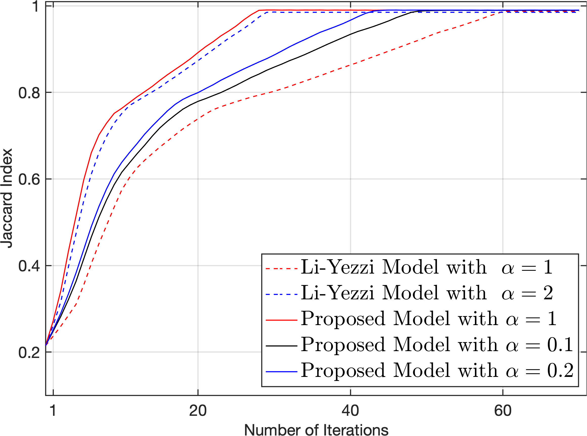
Among the experiments conducted above, we have respectively chosen the parameter to set up the Li-Yezzi dual-front model, and lower values of for the proposed asymmetric dual-front model, in order to demonstrate the advantages of using the introduced asymmetric quadratic metrics. In Fig. 8, we illustrate the comparison results on the convergence rate of both dual-front models, using the test image shown in the first row of Fig. 7. In this experiment, the convergence rates are characterized by the varying Jaccard index values with respect to the number of contour iterations. Even through given lower values of the parameter , one can point out that the convergence rates corresponding to the proposed model (indicated by solid lines) are indeed faster than the Li-Yezzi model (indicated by dash lines), due to the existence of asymmetry penalization encoded in the asymmetric quadratic metrics considered.
Eventually, we evaluate the Li-Yezzi dual-front model, the geodesic distance thresholding model and the proposed asymmetric dual-front model on CT images [69]. In this experiment, the initial contour in each image is a circle centred at an interior point that is farthest to the boundary of the ground truth region in the sense of Euclidean distance. The average values of for the Li-Yezzi model, the geodesic distance thresholding model and the proposed model are respectively , and . Moreover, we exhibit the box plots in Fig. 9 of the statistics of the Jaccard index values from those models. One can claim that the proposed asymmetric dual-front model indeed achieves the highest accuracy among all the compared models. In this experiment, we use the piecewise constant model to set up both dual-front models. We choose for both dual-front models and for the proposed model. Furthermore, a small neighbourhood width is applied in this experiment for both dual-front models, due to the low resolution of the tested CT images. In Fig. 10, we illustrate the image segmentation results, which are produced by the evaluated models on three typical examples sampled from the CT dataset.
Discussion. In the basic formulation of the dual-front scheme, the evolving contour is represented by the interfaces of all adjacent Voronoi regions. The foreground and background segmentation is a fundamental problem, for which the dual-front model can find suitable solutions. Moreover, the multi-region segmentation task can also be efficiently addressed by the dual-front model, as discussed in [50]. We show such an example in Fig. 11 on a synthetic image, where in this case the initial contour is regarded as the union of a series of closed curves, which are depicted by blue lines in Fig. 11a. Fig. 11b shows the the final segmentation contour generated in several contour evolution steps and Fig. 11c illustrates the mean color values in each subregion. Finally, the proposed dual-front model can also be investigated to interactive segmentation on 2D images and 3D volumes based on several user-provided scribbles. These scribbles, each of which can be regarded as a set of points, can provide reliable samples of image features, in order to estimate image data statistics within each subregion. We leave such an interactive segmentation adaption of the proposed dual-front model to the future work.
VI Conclusion
In this paper, we introduce a new dual-front active contour model to address the image segmentation problems. The main contribution of this paper lies at the introduction of asymmetric quadratic metrics to the Voronoi diagram-based dual-front model. As a consequence, the proposed dual-front model is able to blend the benefits from both an asymmetry enhancement and the image region- and edge-based features. The asymmetric features of the considered metrics are derived from the predicted directions, which characterize the motion of the neighbouring offset lines associated to the evolving contour. Contrary to the classical Li-Yezzi model using Riemannian metrics, the introduced dual-front model with asymmetry enhancement is capable of alleviating the shortcut problem, thus can generate more accurate and robust segmentation results in various segmentation scenarios.
Acknowledgment
The authors would like to thank all the anonymous reviewers for their invaluable suggestions to improve this manuscript. This work is in part supported by the National Natural Science Foundation of China (NOs. 61902224, 61906108), by the French government under management of Agence Nationale de la Recherche as part of the “Investissements d’avenir” program, reference ANR-19-P3IA-0001 (PRAIRIE 3IA Institute) and by new AI project towards the integration of education and industry in QLUT (NO. 2020KJC-JC01). The second author’s work was supported by the Wellcome Trust Institutional Strategic Support Award (204909/Z/16/Z). This research is also partially supported by the Young Taishan Scholars (NO.tsqn201909137).
-A Convexity for the Asymmetric Quadratic Metric
We show that the metric with a form of (16) is convex with respect to its second argument .
Proposition 1
Let be a positive definite symmetric matrix and let be a vector, where . Then the following function is convex on .
| (40) |
Proof:
We denote by , where , and are the functions respectively defined as follows:
Clearly the functions , and are convex. Specifically, is non-decreasing, componentwise, on the non-negative quadrant . Moreover, the functions and take non-negative values. The result follows, recalling that the composition of a convex non-decreasing function, with convex functions, defines a convex function, which concludes the proof. ∎
-B Computation for Velocity Functions
Let be a set of simple closed curves which partition the image domain to subregions . Here we denote by a gray level image for or a color image for .
Velocity functions from the region competition model. In the region competition model, the region-based homogeneity property can be described via Gaussian mixture models. In this case, the PDF for the Gaussian mixture model in each region can be expressed as
| (41) |
where and are the weights for the -th Gaussian distribution with parameters . Specifically, represents the mean values of image data within the region , and is the covariance matrix. These parameters can be updated by using the Expectation Maximization algorithm.
With these definitions, the energy functional (9) for the region competition model can be reformulated as
Then the velocity functions for read as
yielding that for any point
For the piecewise constant models [63, 17], the energy functional can be simplified as
where represents the mean intensity value of within the region . In this case, the velocity functions
Then the velocity function can be estimated by Eq. (12).
Velocity functions from Bhattacharyya coefficient. The Bhattacharyya coefficient-based active contour model [27] has proven its strong ability in image segmentation. Basically, this model made use of the Bhattacharyya coefficient between pairs of PDFs or histograms to construct the objective energy functional. In the two-phase segmentation, the contour partitions the image domain into two non-overlapped subregions and , where we suppose is the interior region of . The histogram of image features within each region often relies on a Gaussian kernel , which can be written as
| (42) |
where denotes the area of .
In this case, the Bhattacharyya coefficient can be defined as
| (43) |
where denotes the feature space.
The velocity functions and can be formulated as
| (44) |
and , where the term is defined as
In practice, one can set the kernels to simplify the computation, as discussed in [27].
-C Farthest Point Sampling
We use the Euclidean distance-based farthest point sampling scheme [51] to get a set involving grid points within a given connected region . These points are expected to distribute evenly in as much as possible. For this purpose, we first randomly choose a grid point and initialize the target . Then we extract a point that is farthest to in the sense of Euclidean distance
| (45) |
Once is detected, we update the target set as . One can repeat such a farthest point sampling procedure till the grid point is added to the set .
References
- [1] M. Kass, A. Witkin, and D. Terzopoulos, “Snakes: Active contour models,” Int. J. Comput. Vis., vol. 1, no. 4, pp. 321–331, 1988.
- [2] V. Caselles, F. Catté, T. Coll, and F. Dibos, “A geometric model for active contours in image processing,” Numer. Math., vol. 66, no. 1, pp. 1–31, 1993.
- [3] V. Caselles, R. Kimmel, and G. Sapiro, “Geodesic active contours,” Int. J. Comput. Vis., vol. 22, no. 1, pp. 61–79, 1997.
- [4] R. Malladi, J. Sethian, and B. C. Vemuri, “Shape modeling with front propagation: A level set approach,” IEEE Trans. Pattern Anal. Mach. Intell., vol. 17, no. 2, pp. 158–175, 1995.
- [5] A. Yezzi, S. Kichenassamy, A. Kumar, P. Olver, and A. Tannenbaum, “A geometric snake model for segmentation of medical imagery,” IEEE Trans. Med. Imaging, vol. 16, no. 2, pp. 199–209, 1997.
- [6] L. D. Cohen, “On active contour models and balloons,” CVGIP: Image Understand., vol. 53, no. 2, pp. 211–218, 1991.
- [7] L. D. Cohen and I. Cohen, “Finite-element methods for active contour models and balloons for 2-D and 3-D images,” IEEE Trans. Pattern Anal. Mach. Intell., vol. 15, no. 11, pp. 1131–1147, 1993.
- [8] C. Xu and J. L. Prince, “Snakes, shapes, and gradient vector flow,” IEEE Trans. Image Process., vol. 7, no. 3, pp. 359–369, 1998.
- [9] X. Xie and M. Mirmehdi, “MAC: Magnetostatic active contour model,” IEEE Trans. Pattern Anal. Mach. Intell., vol. 30, no. 4, pp. 632–646, 2008.
- [10] L. D. Cohen and R. Kimmel, “Global minimum for active contour models: A minimal path approach,” Int. J. Comput. Vis., vol. 24, no. 1, pp. 57–78, 1997.
- [11] B. Appleton and H. Talbot, “Globally optimal geodesic active contours,” J. Math. Imaging Vis., vol. 23, no. 1, pp. 67–86, 2005.
- [12] A. K. Mishra, P. W. Fieguth, and D. A. Clausi, “Decoupled active contour (DAC) for boundary detection,” IEEE Trans. Pattern Anal. Mach. Intell., vol. 33, no. 2, pp. 310–324, 2011.
- [13] R. Kimmel and A. M. Bruckstein, “Regularized laplacian zero crossings as optimal edge integrators,” Int. J. Comput. Vis., vol. 53, no. 3, pp. 225–243, 2003.
- [14] J. Melonakos, E. Pichon, S. Angenent, and A. Tannenbaum, “Finsler active contours,” IEEE Trans. Pattern Anal. Mach. Intell., vol. 30, no. 3, pp. 412–423, 2008.
- [15] D. Mumford and J. Shah, “Optimal approximations by piecewise smooth functions and associated variational problems,” Commun. Pure Appl. Math., vol. 42, no. 5, pp. 577–685, 1989.
- [16] S. Zhu and A. Yuille, “Region competition: Unifying snakes, region growing, and Bayes/MDL for multiband image segmentation,” IEEE Trans. Pattern Anal. Mach. Intell., vol. 18, no. 9, pp. 884–900, 1996.
- [17] T. F. Chan and L. A. Vese, “Active contours without edges,” IEEE Trans. Image Process., vol. 10, no. 2, pp. 266–277, 2001.
- [18] T. Brox and D. Cremers, “On local region models and a statistical interpretation of the piecewise smooth Mumford-Shah functional,” Int. J. Comput. Vis., vol. 84, no. 2, pp. 184–193, 2009.
- [19] C. Li, C. Kao, J. C. Gore, and Z. Ding, “Minimization of region-scalable fitting energy for image segmentation,” IEEE Trans. Image Process., vol. 17, no. 10, pp. 1940–1949, 2008.
- [20] L. A. Vese and T. F. Chan, “A multiphase level set framework for image segmentation using the Mumford and Shah model,” Int. J. Comput. Vis., vol. 50, no. 3, pp. 271–293, 2002.
- [21] A. Tsai, A. Yezzi, and A. S. Willsky, “Curve evolution implementation of the Mumford-Shah functional for image segmentation, denoising, interpolation, and magnification,” IEEE Trans. Image Process., vol. 10, no. 8, pp. 1169–1186, 2001.
- [22] X. Bresson, S. Esedoḡlu, P. Vandergheynst, J. Thiran, and S. Osher, “Fast global minimization of the active contour/snake model,” J. Math. Imaging Vis., vol. 28, no. 2, pp. 151–167, 2007.
- [23] A. Chambolle, D. Cremers, and T. Pock, “A convex approach to minimal partitions,” SIAM J. Imaging Sci., vol. 5, no. 4, pp. 1113–1158, 2012.
- [24] L. Grady and C. V. Alvino, “The piecewise smooth Mumford–Shah functional on an arbitrary graph,” IEEE Trans. Image Process., vol. 18, no. 11, pp. 2547–2561, 2009.
- [25] D. Cremers, M. Rousson, and R. Deriche, “A review of statistical approaches to level set segmentation: integrating color, texture, motion and shape,” Int. J. Comput. Vis., vol. 72, no. 2, pp. 195–215, 2007.
- [26] K. Ni, X. Bresson, T. Chan, and S. Esedoglu, “Local histogram based segmentation using the Wasserstein distance,” Int. J. Comput. Vis., vol. 84, no. 1, pp. 97–111, 2009.
- [27] O. Michailovich, Y. Rathi, and A. Tannenbaum, “Image segmentation using active contours driven by the Bhattacharyya gradient flow,” IEEE Trans. Image Process., vol. 16, no. 11, pp. 2787–2801, 2007.
- [28] M. Jung, G. Peyré, and L. D. Cohen, “Nonlocal active contours,” SIAM J. Imaging Sci., vol. 5, no. 3, pp. 1022–1054, 2012.
- [29] B. Sumengen and BS Manjunath, “Graph partitioning active contours (GPAC) for image segmentation,” IEEE Trans. Pattern Anal. Mach. Intell., vol. 28, no. 4, pp. 509–521, 2006.
- [30] W. Zhang, X. Wang, W. You, J. Chen, P. Dai, and P. Zhang, “RESLS: Region and edge synergetic level set framework for image segmentation,” IEEE Trans. Image Process., vol. 29, pp. 57–71, 2019.
- [31] H. Min, W. Jia, Y. Zhao, W. Zuo, H. Ling, and Y. Luo, “LATE: A level-set method based on local approximation of Taylor expansion for segmenting intensity inhomogeneous images,” IEEE Trans. Image Process., vol. 27, no. 10, pp. 5016–5031, 2018.
- [32] G. Sundaramoorthi, A. Yezzi, and . C Mennucci, “Sobolev active contours,” Int. J. Comput. Vis., vol. 73, no. 3, pp. 345–366, 2007.
- [33] C. Li, R. Huang, Z. Ding, J C. Gatenby, D. N Metaxas, and J. C Gore, “A level set method for image segmentation in the presence of intensity inhomogeneities with application to MRI,” IEEE Trans. Image Process., vol. 20, no. 7, pp. 2007–2016, 2011.
- [34] D. Chen, J.-M. Mirebeau, and L. D. Cohen, “Finsler geodesics evolution model for region based active contours,” in Proc. BMVC, 2016.
- [35] D. Chen, J.-M. Mirebeau, and L. D. Cohen, “Global minimum for a Finsler elastica minimal path approach,” Int. J. Comput. Vis., vol. 122, no. 3, pp. 458–483, 2017.
- [36] A. Nakhmani and A. Tannenbaum, “Self-crossing detection and location for parametric active contours,” IEEE Trans. Image Process., vol. 21, no. 7, pp. 3150–3156, 2012.
- [37] S. Osher and J. A. Sethian, “Fronts propagating with curvature-dependent speed: algorithms based on Hamilton-Jacobi formulations,” J. Comput. Phys., vol. 79, no. 1, pp. 12–49, 1988.
- [38] H. Zhao, T. F. Chan, B. Merriman, and S. Osher, “A variational level set approach to multiphase motion,” J. Comput. Phys., vol. 127, no. 1, pp. 179–195, 1996.
- [39] C. Li, C. Xu, C. Gui, and M. D. Fox, “Distance regularized level set evolution and its application to image segmentation,” IEEE Trans. Image Process., vol. 19, no. 12, pp. 3243–3254, 2010.
- [40] V. Estellers, D. Zosso, R. Lai, S. Osher, J.-P. Thiran, and X. Bresson, “Efficient algorithm for level set method preserving distance function,” IEEE Trans. Image Process., vol. 21, no. 12, pp. 4722–4734, 2012.
- [41] R. Saye and J. A. Sethian, “Analysis and applications of the Voronoi implicit interface method,” J. Comput. Phys., vol. 231, no. 18, pp. 6051–6085, 2012.
- [42] T. F. Chan, S. Esedoglu, and M. Nikolova, “Algorithms for finding global minimizers of image segmentation and denoising models,” SIAM J. Appl. Math., vol. 66, no. 5, pp. 1632–1648, 2006.
- [43] E. Bae, J. Yuan, and X.-C. Tai, “Global minimization for continuous multiphase partitioning problems using a dual approach,” Int. J. Comput. Vis., vol. 92, no. 1, pp. 112–129, 2011.
- [44] A. Chambolle and T. Pock, “A first-order primal-dual algorithm for convex problems with applications to imaging,” J. Math. Imaging Vis., vol. 40, no. 1, pp. 120–145, 2011.
- [45] T. Goldstein, X. Bresson, and S. Osher, “Geometric applications of the split bregman method: segmentation and surface reconstruction,” J. Sci. Comput., vol. 45, no. 1-3, pp. 272–293, 2010.
- [46] P. A. Arbeláez and L. D Cohen, “Energy partitions and image segmentation,” J. Math. Imaging Vis., vol. 20, no. 1, pp. 43–57, 2004.
- [47] X. Bai and G. Sapiro, “Geodesic matting: A framework for fast interactive image and video segmentation and matting,” Int. J. Comput. Vis., vol. 82, no. 2, pp. 113–132, 2009.
- [48] D. Chen, J. Spencer, J.-M. Mirebeau, K. Chen, and L. Cohen, “Asymmetric geodesic distance propagation for active contours,” in Proc. BMVC, 2018.
- [49] H. Li and A. Yezzi, “Local or global minima: Flexible dual-front active contours,” IEEE Trans. Pattern Anal. Mach. Intell., vol. 29, no. 1, pp. 1–14, 2007.
- [50] A. Dubrovina-Karni, G. Rosman, and R. Kimmel, “Multi-region active contours with a single level set function,” IEEE Trans. Pattern Anal. Mach. Intell., vol. 37, no. 8, pp. 1585–1601, 2015.
- [51] G. Peyré and L. D Cohen, “Geodesic remeshing using front propagation,” Int. J. Comput. Vis., vol. 69, no. 1, pp. 145, 2006.
- [52] S. Bougleux, G. Peyré, and L. D. Cohen, “Anisotropic geodesics for perceptual grouping and domain meshing,” in Proc. ECCV, 2008, pp. 129–142.
- [53] G. Leibon and D. Letscher, “Delaunay triangulations and Voronoi diagrams for Riemannian manifolds,” in Proc. Annual Symposium on Computational Geometry, 2000, pp. 341–349.
- [54] G. Peyré, M. Péchaud, R. Keriven, and L. D. Cohen, “Geodesic methods in computer vision and graphics,” Foundations and Trends® in Computer Graphics and Vision, vol. 5, no. 3–4, pp. 197–397, 2010.
- [55] J.-M. Mirebeau, “Anisotropic fast-marching on cartesian grids using lattice basis reduction,” SIAM J. Numer. Anal., vol. 52, no. 4, pp. 1573–1599, 2014.
- [56] J.-M. Mirebeau, “Efficient fast marching with Finsler metrics,” Numer. Math., vol. 126, no. 3, pp. 515–557, 2014.
- [57] J.-M. Mirebeau, “Riemannian fast-marching on cartesian grids, using voronoi’s first reduction of quadratic forms,” SIAM J. Numer. Anal., vol. 57, no. 6, pp. 2608–2655, 2019.
- [58] L. Bertelli, B. Sumengen, BS Manjunath, and F. Gibou, “A variational framework for multiregion pairwise-similarity-based image segmentation,” IEEE Trans. Pattern Anal. Mach. Intell., vol. 30, no. 8, pp. 1400–1414, 2008.
- [59] R. Duits, S. P. L. Meesters, J.-M. Mirebeau, and J. M. Portegies, “Optimal paths for variants of the 2D and 3D Reeds–Shepp car with applications in image analysis,” J. Math. Imag. Vis., vol. 60, no. 6, pp. 816–848, 2018.
- [60] S. Di Zenzo, “A note on the Gradient of a Multi-Image,” Comput. Vis. Graph. Image Process., vol. 33, no. 1, pp. 116–125, 1986.
- [61] N. Sochen, R. Kimmel, and R. Malladi, “A general framework for low level vision,” IEEE Trans. Image Process., vol. 7, no. 3, pp. 310–318, 1998.
- [62] C. Li, J. Liu, and M. D. Fox, “Segmentation of edge preserving gradient vector flow: an approach toward automatically initializing and splitting of snakes,” in Proc. CVPR). IEEE, 2005, vol. 1, pp. 162–167.
- [63] T. F. Chan, B. Y. Sandberg, and L. A. Vese, “Active contours without edges for vector-valued images,” J. Vis. Commun. Image Represent., vol. 11, no. 2, pp. 130–141, 2000.
- [64] J.-M. Mirebeau, “Fast-marching methods for curvature penalized shortest paths,” J. Math. Imag. Vis., vol. 60, no. 6, pp. 784–815, 2018.
- [65] J. A. Sethian, “Fast marching methods,” SIAM Review, vol. 41, no. 2, pp. 199–235, 1999.
- [66] J.-M. Mirebeau and J. Portegies, “Hamiltonian fast marching: a numerical solver for anisotropic and non-holonomic eikonal PDEs,” Image Processing On Line, vol. 9, pp. 47–93, 2019.
- [67] C. Rother, V. Kolmogorov, and A. Blake, “Grabcut: Interactive foreground extraction using iterated graph cuts,” ACM Trans. Graph., vol. 23, no. 3, pp. 309–314, 2004.
- [68] R. Malladi and J. A. Sethian, “A real-time algorithm for medical shape recovery,” in Proc. ICCV, 1998, pp. 304–310.
- [69] J. Spencer, K. Chen, and J. Duan, “Parameter-free selective segmentation with convex variational methods,” IEEE Trans. Image Process., vol. 28, no. 5, pp. 2163–2172, 2019.