Model Based Screening Embedded Bayesian Variable Selection for Ultra-high Dimensional Settings
Abstract
We develop a Bayesian variable selection method, called SVEN, based on a hierarchical Gaussian linear model with priors placed on the regression coefficients as well as on the model space. Sparsity is achieved by using degenerate spike priors on inactive variables, whereas Gaussian slab priors are placed on the coefficients for the important predictors making the posterior probability of a model available in explicit form (up to a normalizing constant). The strong model selection consistency is shown to be attained when the number of predictors grows nearly exponentially with the sample size and even when the norm of mean effects solely due to the unimportant variables diverge, which is a novel attractive feature. An appealing byproduct of SVEN is the construction of novel model weight adjusted prediction intervals. Embedding a unique model based screening and using fast Cholesky updates, SVEN produces a highly scalable computational framework to explore gigantic model spaces, rapidly identify the regions of high posterior probabilities and make fast inference and prediction. A temperature schedule guided by our model selection consistency derivations is used to further mitigate multimodal posterior distributions. The performance of SVEN is demonstrated through a number of simulation experiments and a real data example from a genome wide association study with over half a million markers.
Key words: GWAS, hierarchical model, posterior prediction, shrinkage, spike and slab, stochastic search, subset selection.
1 Introduction
In almost every scientific discipline, rapid collection of sophisticated data has been booming due to recent advancements in technology. In biology, for example, automated sequencing tools have made whole genome sequencing possible in a cost effective manner, thus providing variations of millions of single nucleotides between individuals. On the other hand, because phenotypic data are typically collected via carefully conducted scientific experiments or other observational studies, number of observations remains on the smaller size, giving rise to regression problems where the number of variables far exceeds the sample size . Nevertheless, only a few of these variables are believed to be associated with the response. Thus, variable selection plays a crucial role in the modern scientific discoveries.
Classical approaches to deal with the variable selection problems are through regularization methods. A variety of methods using different penalization techniques have been proposed for variable selection in the linear models, such as the lasso (Tibshirani 1996; Datta and Zou 2017), SCAD (Fan and Li 2001; Kim et al. 2008), elastic net (Zou and Hastie 2005), adaptive lasso (Zou 2006), the octagonal shrinkage and clustering algorithm for regression (Bondell and Reich 2008), L0-penalty for best subset regression (Bertsimas et al. 2016; Huang et al. 2018) and others. These methods achieve sparsity by either penalizing the effect sizes or the model sizes but rarely both. Several Bayesian variable selection methods exploit the connection between the penalized estimators and the modes of Bayesian posterior densities under suitably chosen prior distributions on the regression coefficients. Example includes the lasso-Laplace prior connection (Tibshirani 1996), the hierarchical Bayesian lasso (Park and Casella 2008) and other works by Kyung et al. 2010, Xu and Ghosh 2015 and Roy and Chakraborty 2017.
Another popular approach to Bayesian variable selection is integrating the penalties on the effect size and the model size via priors distributions. To that end, auxiliary indicator variables indicating the presence or absence of each variable are introduced to obtain a ‘spike and slab’ prior on the regression coefficients. Here the ‘spike’ corresponds to the probability mass concentrated at zero or around zero for the variables vulnerable to deletion and the ‘slab’ specifies prior uncertainty for coefficients of other variables. Analysis using such models determines (selects) the most promising variables by summarizing the posterior density of the indicator variables and/or the regression coefficients. The seminal works of Mitchell and Beauchamp 1988; George and McCulloch 1993; George and McCulloch 1997 developed a hierarchy of priors over the regression coefficients and the latent indicators and used Gibbs sampler to identify promising models in low dimensional setup (Yuan and Lin 2005; Ishwaran and Rao 2005; Liang et al. 2008; Johnson and Rossell 2012, see also). Several of these methods have been recently modified and extended to the ultra-high dimensional setup. Narisetty and He 2014 pioneered the theoretical study of Bayesian variable selection in the ultra-high dimensional setup, Ročková and George 2014 introduced the EM algorithm for fast exploration of high-posterior models, Yang et al. 2016 studied model selection consistency and computational complexity when -prior is placed on the regression coefficients, Shin et al. 2018 extended the popular non-local priors to model selection and modified the stochastic shotgun model search algorithm (Hans et al. 2007), while Zhou and Guan 2019 and Zanella and Roberts 2019 implemented Metropolis Hastings algorithms with an iterative complex factorization and a tempered Gibbs sampler, respectively, for estimating posterior model probabilities.
From a practical standpoint, in the ultra-high dimensional set up, where the number of variables () is much larger than the sample size (), generally variable screening is performed to reduce the number of variables before applying any of the aforementioned variable selection methods for choosing important variables. The classical approaches as well as Narisetty and He 2014 resort to a two stage procedure where they first use frequentist screening algorithms (Fan and Lv 2008; Wang and Leng 2016) to reduce the dimension of the problem and then perform variable selection. Shin et al. 2018 as well as Cao et al. 2020 fuse the frequentist iterated sure independent screening in their stochastic search algorithm. However, these screening methods are frequentist procedures that are not guaranteed to be fidelitous to the Bayesian model in practice.
In this work, we extend the classical variable selection model of Mitchell and Beauchamp 1988 to the ultra-high dimensional setting. Following the path laid by Narisetty and He 2014 we derive posterior consistency results. By considering zero (exact spike) inflated mixture priors for regression coefficients, we are able to introduce sparsity and relax some assumptions of Narisetty and He 2014. Furthermore, we develop a novel methodology for variable selection in the spirit of the stochastic shotgun search algorithm (Hans et al. 2007) with embedded screening that is faithful to the hierarchical Bayesian model. We develop sophisticated computational framework that allows us to consider larger search neighborhoods and compute exact unnormalized posterior probabilities in contrast to Shin et al. 2018. Furthermore, in order to recover models with large posterior probabilities and mitigate posterior multimodality associated with variable selection models, we use a temperature schedule that is guided by our posterior model selection consistency asymptotics. We call this Bayesian method and the computational framework election of ariables with mbedded screeing (SVEN). Keeping prediction of future observations in mind, we develop novel methods for computing approximate posterior predictive distribution and prediction intervals. In particular, using SVEN we construct two prediction intervals, called Z-prediction intervals and Monte Carlo prediction intervals.
The rest of the paper is laid out as follows. In Section 2 we describe the hierarchical Bayesian variable selection model and prove strong model selection consistency results (Section 2.1); develop the SVEN framework (Section 2.2) and prediction methods (Section 3). We perform detailed simulation studies in Section 4 and compare our methods to several other popular Bayesian and frequentist methods. In Section 5 we analyze a massive dataset from an agricultural experiment with and where among the Bayesian methods used for comparison only our method is able to perform variable selection on the whole data. We also show the practical usefulness of our method in obtaining posterior predictive distribution and prediction intervals for the yield of novel crop varieties. We conclude in Section 6 with some discussion and future research directions. A supplement document containing the proofs of the theoretical results and some computational details is available with sections referenced here with the prefix ‘S’. The methodology proposed here is implemented in an accompanying R package ‘bravo’ for ayesian sceening nd ariable selectin.
2 Bayesian variable selection with screening
2.1 Hierarchical mixture models
2.1.1 Model description
Let denote a vector of response values, an design matrix of potential predictors, with vector of partial regression coefficients We assume latent indicator vector to denote a model such that the th predictor is included in the regression model if and and only if . Corresponding to the binary vector, the size of a model is denoted as , where . Also, with model , let be the sub-matrix of that consists of columns of corresponding to model and be the vector that contains the regression coefficients for model . In the first hierarchy of the Bayesian hierarchical mixture model we assume that the conditional distribution of given and is -dimensional Gaussian and is given by
| (1) |
where is the intercept term and is the conditional variance. Thus (1) indicates that each corresponds to a Gaussian linear regression model where the residual vector However, because the original covariates could have unbalanced scales, a common approach is to reparameterize the above model using a scaled covariate matrix. To that end, suppose is the vector of column means of and is the diagonal matrix whose th diagonal entry is the sample standard deviation of (the th column of ) and let denote the scaled covariate matrix. Also we assume that and The Bayesian hierarchical regression model after reparameterization is given by
| (2a) | ||||
| (2b) | ||||
| (2c) | ||||
| (2d) | ||||
In this hierarchical setup a popular non-informative prior is set for in (2c) and a conjugate independent normal prior is used on given in (2b) with controlling the precision of the prior independently from the scales of measurements. Note that under this prior, if a covariate is not included in the model, the prior on the corresponding regression coefficient degenerates at zero. In (2d) an independent Bernoulli prior is set for , where reflects the prior inclusion probability of each predictor. We assume and are known non-random functions of and
The hierarchical model (2) with centered allows us to obtain the distribution of given in a closed form by integrating out and (Roy et al. 2018, section S6). Consequently, the marginal likelihood function of is given by
| (3) |
where is the determinant of
| (4) |
is the ridge residual sum of squares, , and is the normalizing constant.
In order to identify the important variables, we use the (marginal) posterior distribution of . Thanks to the explicit form of the marginal likelihood (2.1.1), this posterior density is given by
It’s often convenient to work with log of the posterior density which is given by
| (5) |
Remark 1.
Remark 2.
Remark 3.
As an alternative to the independent normal prior (2b), it is also possible to consider Zellner’s -prior (Zellner 1986) on given by provided that for every all submatrices of have full column rank and we restrict the support of the prior distribution on to models of size at most Assuming that is a non-random function of and the marginal posterior of is then given by
where the priors on and have been assumed to be the same as (2c).
Ideally, as the sample size increases we would like the posterior of to concentrate more and more on the important variables. Several works have alluded to asymptotic guarantees for strong model selection consistency in the ultra-high dimensional regression where is allowed to vary subexponentially with i.e. and Here, the strong model selection consistency implies that the posterior probability of the true set of variables converge to 1 as tends to infinity. Under shrinking and diffusing priors, Narisetty and He 2014 developed explicit scaling laws for hyper-parameters that are sufficient for strong model selection consistency. On the other hand, Shin et al. 2018, and more recently, Cao et al. 2020 established sufficient conditions for strong model selection consistency under non-local type priors (Johnson and Rossell 2012). The Bayesian hierarchical model (2) is similar to Narisetty and He 2014’s (Narisetty and He 2014) model with the crucial distinction that the spike prior is degenerate: Consequently, although most assumptions used here for selection consistency are similar to those made by Narisetty and He 2014, we are able to relax some of the conditions to allow for more noisy unimportant variables. In the next section we describe strong model selection consistency results for (2).
2.1.2 Model selection consistency
We consider the ultra-high dimensional setting where the number of variables is allowed to vary subexponentially with the sample size. As established by Narisetty and He 2014 the slab precision also needs to vary with for strong model selection consistency. In order to state the assumptions and the main results, we use the following notations. Abusing notation, we interchangeably use a model either as a -dimensional binary vector or as a set of indices of non-zero entries of the binary vector. For models and denotes the complement of the model , and and denote the union and intersection of and , respectively. For two real sequences and , means for some constant ; (or ) means ; (or ) means . Also for any matrix , let and denote its minimum and maximum eigenvalues, respectively, and let be its minimum nonzero eigenvalue. Again, abusing notations, for two real numbers and , and denote max and min respectively. Define and for , where
Finally for any fixed positive integer , define
where is the orthogonal projection matrix onto the column space of and denotes the norm. Here, denotes the Moore-Penrose inverse of . We assume the following set of conditions.
C 1.
for some as , that is, .
C 2.
for some , and .
C 3.
where the true model is fixed and .
C 4.
For given in C2, there exists such that , and for some ,
.
C 5.
For some positive constants and
The condition C2 states that the conditional distribution of given is diffused in the sense that it’s conditional prior variance goes to infinity at a particular rate. The condition C3 greatly relaxes the boundedness assumption on in Narisetty and He 2014, by slightly strengthening the identifiability condition C4. Yang et al. 2016 obtained similar results under -priors on but as mentioned by them our independence prior is ‘a more realistic choice’. Moreover, Yang et al. 2016 assumed that is bounded away from zero for all models of size at most which is unrealistic because, for example, even when entries of are iid N(0,1), converges to zero in probability. Because of the degenerated form of the spike priors, the regularity assumptions on the submatrices of the design matrix in C4 relax the assumptions on the bound on their largest eigenvalues. Narisetty and He 2014 showed that if the rows of are independent isotropic sub-Gaussian random vectors then C4 holds with overwhelmingly large probability (Chen and Chen 2008; Kim et al. 2012; Shin et al. 2018, see also). The regularity assumption for the true model C5 is standard and has been used in both Narisetty and He 2014 and Cao et al. 2020 without being explicitly stated.
Note that the condition C3 does not explicitly specify the true model and the relaxation to allow higher noise warrants a validation of the identifiability of . To that end, suppose on the contrary that it is possible to include some variables, say from into the true model and still maintain the conditions C1-C5 for both and as true models for every Then condition C4 with (now excluding the apparently true variable ) would imply Here, the first equality follows from the fact that . But because is symmetric and idempotent,
| (6) |
However, condition C3 for implies This with (6) implies that
which contradicts condition C3. We now present the strong model selection consistency results.
Theorem 1.
Assume conditions C1–C5 hold and that is known. Then the posterior probability of the true model, in probability as the sample size approaches .
Proof.
The proof is given in Section S4 of the supplementary materials. ∎
Note that the statement of Theorem 1 is equivalent to in probability as The proof of Theorem 1 also provides the rate of convergence given by,
with probability greater than for some positive constants , , , , and , where It is encouraging that despite relaxing the boundedness condition on , the rate of convergence remains the same as in Narisetty and He 2014.
However, in practice is typically never known. In this case, we need a further assumption that assigns a prior probability of zero on for some .
C 6.
For some and , .
This condition is same as in Narisetty and He 2014 and also equivalent to the assumptions on the prior model sizes in Shin et al. 2018 and Cao et al. 2020.
Theorem 2.
Assume conditions C1–C6 hold. Then the posterior probability of the true model, in probability as the sample size approaches .
Proof.
The proof is given in Section S5 of the supplementary materials. ∎
Note that strong consistency results also imply that with probability tending to one, the true model is the posterior mode, that is, as However, in finite sample this need not be true. Furthermore, when the regularity conditions do not hold, there may be multiple models with large posterior probabilities even for large . Thus, we would like to discover models with practically large posterior probability values. However, in ultra-high dimensional problems, traditional computational methods based on Markov chain Monte Carlo (MCMC) algorithms have poor performance. Thus next we describe SVEN to explore the posterior distribution In particular, SVEN will be used to discover high probability regions and find the maximum a posteriori (MAP) model .
2.2 Searching for high posterior probability models
2.2.1 Stochastic shotgun search algorithms
Hans et al. 2007 proposed the stochastic shotgun search (SSS) algorithm for recovering models with large posterior probabilities. To that end, for a given model let denote a neighborhood of , where is an “added” set containing all the models with one of the remaining covariates added to the current model , is a “deleted” set obtained by removing one variable from and is a “swapped” set containing the models with one of the variables from replaced by one variable from The SSS algorithm then starts with an initial model and for
- -
(SSS1) Compute for all nbd().
- -
(SSS2) Separately sample from from and from with probabilities proportional to
- -
(SSS3) Sample from and with probability proportional to and respectively.
After running for some prespecified large number of iterations, the algorithm then declares the model discovered with the largest (unnormalized) posterior probability as the MAP model. Hans et al. 2007 notes that the sampling probabilities in (SSS1) and (SSS2) can be replaced by the Bayesian information criteria (BIC) and the sampling weights can be computed in parallel.
Following the success of SSS, Shin et al. 2018 propose further improvement. Note that, Shin et al. 2018 use non-local priors, and so the posterior probabilities are not available analytically. In fact, they resort to using computationally expensive Laplace approximation which suggests exact numerical computations of these quantities are also not straightforward (Cao et al. 2020, see also). Also in ultra-high dimensional problems, SSS may not be scalable due to its implementation. Thus Shin et al. 2018 propose a simplified stochastic shotgun search with screening (S5) by dropping the “swapped” set from consideration and moreover, by screening out variables from the “added” set. (Note that, in high dimension, the number of “swapped” models is much larger than the numbers of “added” and “deleted” models.) For screening, borrowing ideas from frequentist correlation screening of Fan and Lv 2008, they propose computing the least squares residuals from a regression of on and compute the absolute correlations between each column of and the residuals. They then propose keeping models in the “added” set corresponding to the largest few of the absolute correlations. This greatly reduces the burden of computing for all in the “added” set. However, in their R package BayesS5, the authors have used ridge residuals with unit ridge penalty instead of the least squares residuals. Nevertheless, the S5 algorithm has been useful for exploring the posterior distribution of (Cao et al. 2020).
In the variable selection model (2), the Gaussian conjugacy provides analytically tractable forms for up to a normalizing constant. We also show that can be rapidly computed for the swapped models, thereby allowing us to include the swapped models in the neighborhood. We thus develop a stochastic shotgun algorithm with (posetrior) model based screening and develop scalable statistical computations for drawing fast Bayesian inference and prediction.
2.2.2 Selection of variables with embedded screening
In order to describe the SVEN algorithm, we first describe how to compute the unnormalized posterior probabilities in the (SSS1) step. To that end, compute as once and for all. Next, suppose we have a current model and we want to compute the posterior probabilities of each model in Suppose is the upper triangular Cholesky factor of and In the algorithm below, scalar addition to vector, division between two vectors and other arithmetical and algebraic operation on vectors are interpreted as entry-wise operations, as implemented in most statistical software (e.g. in R). Then
- 1.
Compute by using forward substitution.
- 2.
Update [No need to center Z because ]
- 3.
Compute as the sum of squares of each column of Note that is a matrix and so these sums of squares should be computed without storing another matrix.
- 4.
Set where the arithmatical operations are performed entrywise on the vector. Also in this operation, the entries corresponding to the variables in are ignored.
- 5.
Compute
- 6.
Compute
- 7.
Compute
- 8.
Compute
Then for all the th entry of above contains the unnormalized posterior probability of the model obtained by including in The other entries are ignored. For each model in its posterior probability can be computed easily because typically is small. Furthermore, for each we can use the above algorithm to compute the unnormalized posterior probabilities of in Thus we can compute the (unnormalized) posterior probabilities of each model in nbd
Given the current model , the complexity for computing (unnormalized) for all nbd by the above algorithm is , where denotes the number of non-zero elements in . Since is practically finite, the computational complexity is simply . If in addition, is sparse, as in the genome-wide association study example in section 5, the complexity for computing all posterior probabilities in nbd is linear in both and . Finally, note that, the additional memory requirement for the above algorithm except storing the matrix is practically . Also, different steps including step 2 of the above algorithm can be performed in parallel using distributed computing architecture.
Using the above algorithm as the foundation, we now discuss the SVEN algorithm. Suppose is a given temperature schedule. Let denote the empty model (i.e. the model without any predictor included). Then, for
- -
Set to be the empty model. Then for
- -
(SVEN1) [Same as (SSS1)] Compute for all nbd
- -
(SVEN2) [Screening step] Consider at most 20 highest probability neighboring models. That is, construct the set nbd with such that only if
and where is some prespecified number (we use ).
- -
(SVEN3) [Shotgun step] Assign the weight to a model Sample a model from using these weights and set it as
Our ability to efficiently compute posterior probability of all neighboring models allows us to implement the screening (SVEN2) directly using the objective function . This is a key difference between SVEN and S5 of Shin et al. 2018. Because models with large probabilities could be separated by models with very low probabilities, a temperature schedule has been used. Such tempering is quite common in simulated annealing (Kirkpatrick et al. 1983) and has also been used in Shin et al. 2018. In order to choose a temperature schedule, we turn to our asymptotic results from Section S4. In particular, the theory indicates that the log-posterior probabilities of good models with small model size are separated by roughly Thus in order to facilitate jumps between these models we set where the additional is a heuristic adjustment common in numerical computations. Also the remaining temperatures are chosen to be equally spaced between 1 and
Note that at every temperature we start the SVEN algorithm at the empty model that are run separately. Because the stochastic shotgun might have a tendency to wander off to obscure valleys containing large number of variables especially under high temperature; running them separately avoids getting trapped in such a valley. Most good models have small size and so they could be explored relatively early when started multiple times from the empty model.
Note that our algorithm does not require explicitly storing the matrix Indeed, in many applications, could be sparse and efficiently stored in the memory. The matrix on the other hand is always dense. Overall our method is extremely memory efficient, and we are able to directly perform variable selection with significantly larger than the other methods may handle.
In addition to the MAP model, our method also provides the posterior probability of all the models explored by the algorithm and facilitate approximate Bayesian model averaging (Shin et al. 2018). To that end, we sort the models according to decreasing posterior probabilities and retain the best (highest probability) models where is chosen so that where is a prespecified tolerance (we use ). Then we assign the weights
| (7) |
to the model We define the approximate marginal inclusion probabilities for the th variable as and define the weighted average model (WAM) as the model containing variables with Note that if SVEN is allowed to run indefinitely to explore all models and is set as zero, then the WAM would be theoretically identical to the median probability model (Barbieri and Berger 2004). However, computing the median probability model is infeasible when because enumerating all the posterior probabilities of is practically impossible.
In the literature, mostly the MAP (more precisely the discovered MAP model) model is used for prediction. In the next section we develop methods for point and interval predictions using the top models ’s with associated weights ’s.
3 Posterior predictive distribution and intervals
The posterior predictive distribution of the response at a new covariate vector conditional on the observed covariate matrix and hyper-parameters and is given by,
| (8) |
where is the density of as given in (1), is the joint posterior density of given deduced from the hierarchical model (2), and . Note that, the distribution (8) is not tractable. However, as shown later in this section, posterior predictive mean and variance of can be expressed as (posterior) expectations of some analytically available functions of . Also, samples from an approximation of (8) can be drawn using our SVEN algorithm. Using these approaches, we now propose two methods for computing approximate posterior prediction intervals for
3.1 A Z-prediction interval
In this section we describe some approximations to and and use those to construct an interval for . To that end, from (2) we observe that and are conditionally independent given and with
| (9) |
where as defined in section 2.1.1. Consequently, the full conditional distribution of is a -dimensional multivariate Gaussian distribution given by
| (10) |
where and are sub-vector of and sub-matrix of , respectively corresponding to the model , and Also,
| (11) |
where denotes a inverse gamma random variable with density , and is defined in (4). Next, let and note that . Thus, using iterated expectation and variance formulas, we have
| (12a) | ||||
| (12b) | ||||
From (12a) and (12b) we see that both and can be expressed as posterior expectations of analytically available functions of . However, because the posterior of is not entirely available, we propose using the models obtained from SVEN as described in section 2.2.2 with weights respectively, to approximate these expectations and variances. We can use these approximate posterior predictive mean and variance of to obtain a prediction interval for as where is the th standard normal quantile. We call this interval Z-prediction interval (Z-PI). Also, the posterior predictive mean is used as a point estimate of . In the next section, we describe an alternative method for computing a prediction interval for using Monte Carlo simulation.
3.2 A Monte Carlo prediction interval
A prediction interval for can also be constructed using Monte Carlo (MC) samples generated from the posterior predictive distribution (8). Specifically, a prediction interval for is given by where denotes the -th quantile of the distribution (8). Now, we describe a method for sampling from an approximation of (8) using SVEN. To that end, we consider given by
| (13) |
where ’s are defined in (7), and are the highest probability models obtained by SVEN as described in section 2.2.2. Thus, is the posterior predictive pdf given in (8) except that the marginal posterior of is replaced by a mixture distribution of models chosen by SVEN. Samples from (13) can be drawn as follows. First, we sample from the top models with Given we then sample from (11). Next given and we sample and from (9). Then we compute and , which are samples from (10). Finally generate from We repeat the above process a large number of times and construct a MC prediction interval (MC-PI) for as where denotes the empirical quantiles based on these samples. In practice, generally one wants prediction intervals at several new covariate vectors ’s. In section S1 of the supplementary materials, we describe a computationally efficient way of drawing multiple samples from (13) using the above method and thus simultaneously computing prediction intervals at several new covariate vectors ’s.
4 Simulation studies
In this section, we study the performance of our SVEN method through several numerical experiments, and compare it with some other existing methods. The competing variable selection methods we consider are S5 (R package: BayesS5), EMVS (R package: EMVS), fastBVSR and three penalization methods, LASSO, Elastic Net with elastic mixing parameter (R package: glmnet) and SCAD (R package: ncvreg). As also noted in Shin et al. 2018, we could not include BASAD (Narisetty and He 2014) for its high computational burden and our ultra-high dimensional examples. As used in Table 1 of Ročková and George 2014 we run EMVS with and three choices for namely, (EMVS1), (EMVS2) and (EMVS3). For fastBVSR, the results are obtained using 100,000 MCMC iterations after a burn-in of 10,000 steps. For S5 the hyperparameters are tuned using a function provided in BayesS5. Moreover, we denote by piMOM and peMOM, respectively, the product inverse-moment and the product exponential moment non-local priors used under S5. In addition, for piMOM and peMOM, we use MAP and LS to denote the MAP estimator and the least squares estimator from the MAP model, respectively. Under SVEN, both MAP and WAM models, as described in section 2.2 are considered. For SVEN, we use and the temperature schedule described in Section 2.2.2 with Also, for SVEN, the ridge estimator is used to estimate the regression coefficients for the MAP and the WAM models.
4.1 Setup of experiments
Our numerical studies are conducted in six different simulation settings described below.
4.1.1 Independent predictors
In this example, entries of are generated independently from . The coefficients are specified as and
| Method | MSPE | MSEβ | Coverage probability (%) | Average model size | FDR (%) | FNR (%) | Jaccard Index (%) |
|---|---|---|---|---|---|---|---|
| SVEN(WAM) | 0.6387 | 0.0083 | 100 | 5 | 0 | 0 | 100 |
| SVEN(MAP) | 0.6387 | 0.0083 | 100 | 5 | 0 | 0 | 100 |
| piMOM(MAP) | 0.6384 | 0.0081 | 100 | 5 | 0 | 0 | 100 |
| peMOM(MAP) | 0.6384 | 0.0080 | 100 | 5 | 0 | 0 | 100 |
| piMOM(LS) | 0.6387 | 0.0083 | 100 | 5 | 0 | 0 | 100 |
| peMOM(LS) | 0.6387 | 0.0083 | 100 | 5 | 0 | 0 | 100 |
| fastBVSR | 0.6478 | 0.0091 | 100 | 5.09 | 1.45 | 0 | 98.55 |
| EMVS1 | 1.0087 | 0.3777 | 0 | 3.80 | 0 | 24 | 76 |
| EMVS2 | 2.5203 | 1.8734 | 0 | 1.99 | 0 | 60.2 | 39.8 |
| EMVS3 | 5.0909 | 4.3994 | 0 | 0.53 | 0 | 89.4 | 10.6 |
| LASSO | 0.7489 | 0.1146 | 100 | 56.5 | 87.34 | 0 | 12.66 |
| SCAD | 0.6454 | 0.0152 | 100 | 18.42 | 47.50 | 0 | 52.50 |
| Elastic Net | 0.8266 | 0.1898 | 100 | 91.15 | 93.08 | 0 | 6.92 |
| Method | MSPE | MSEβ | Coverage probability (%) | Average model size | FDR (%) | FNR (%) | Jaccard Index (%) |
|---|---|---|---|---|---|---|---|
| SVEN(WAM) | 48.3069 | 1.1912 | 100 | 5 | 0 | 0 | 100 |
| SVEN(MAP) | 48.3069 | 1.1892 | 100 | 5 | 0 | 0 | 100 |
| piMOM(MAP) | 48.2277 | 1.0018 | 100 | 5 | 0 | 0 | 100 |
| peMOM(MAP) | 50.1528 | 3.5669 | 94 | 4.96 | 0.37 | 1.2 | 98.5 |
| piMOM(LS) | 48.3069 | 1.1892 | 100 | 5 | 0 | 0 | 100 |
| peMOM(LS) | 50.2789 | 3.8758 | 94 | 4.96 | 0.37 | 1.2 | 98.5 |
| fastBVSR | 50.0479 | 2.5620 | 100 | 5.78 | 9.54 | 0 | 90.46 |
| EMVS1 | 50.7090 | 7.0499 | 100 | 5.63 | 9.22 | 0 | 90.78 |
| EMVS2 | 49.9839 | 5.3218 | 100 | 5.26 | 4.14 | 0 | 95.86 |
| EMVS3 | 49.6243 | 4.5157 | 100 | 5.08 | 1.33 | 0 | 98.67 |
| LASSO | 55.2280 | 17.9975 | 100 | 51.02 | 89.94 | 0 | 8.44 |
| SCAD | 48.3167 | 1.2556 | 100 | 6.29 | 11.55 | 0 | 88.45 |
| Elastic Net | 57.5750 | 23.9724 | 100 | 89.68 | 93.76 | 0 | 6.24 |
| Method | MSPE | MSEβ | Coverage probability (%) | Average model size | FDR (%) | FNR (%) | Jaccard Index (%) |
|---|---|---|---|---|---|---|---|
| SVEN(WAM) | 2.1521 | 0.0173 | 100 | 3 | 0 | 0 | 100 |
| SVEN(MAP) | 2.1521 | 0.0173 | 100 | 3 | 0 | 0 | 100 |
| piMOM(MAP) | 2.1519 | 0.0172 | 100 | 3 | 0 | 0 | 100 |
| peMOM(MAP) | 2.1515 | 0.0168 | 100 | 3 | 0 | 0 | 100 |
| piMOM(LS) | 2.1521 | 0.0173 | 100 | 3 | 0 | 0 | 100 |
| peMOM(LS) | 2.1521 | 0.0173 | 100 | 3 | 0 | 0 | 100 |
| fastBVSR | 2.1961 | 0.0187 | 100 | 3.03 | 0.75 | 0 | 99.25 |
| EMVS1 | 2.2738 | 0.1286 | 100 | 6.7 | 54.57 | 0 | 45.43 |
| EMVS2 | 2.2803 | 0.1419 | 100 | 5.28 | 41.42 | 0 | 58.58 |
| EMVS3 | 2.2947 | 0.1619 | 100 | 4.33 | 28.40 | 0 | 71.60 |
| LASSO | 2.3118 | 0.1641 | 100 | 28.16 | 76.82 | 0 | 23.19 |
| SCAD | 2.1592 | 0.0252 | 100 | 10.33 | 28.30 | 0 | 71.70 |
| Elastic Net | 2.4590 | 0.3754 | 100 | 54.35 | 91 | 0 | 9.00 |
| Method | MSPE | MSEβ | Coverage probability (%) | Average model size | FDR (%) | FNR (%) | Jaccard Index (%) |
| SVEN(WAM)4 | 78.7067 | 299.4512 | 0 | 2.65 | 0 | 82.33 | 17.67 |
| SVEN(MAP)4 | 81.0355 | 533.5387 | 0 | 3 | 0 | 80 | 20 |
| SVEN(WAM)5 | 82.5443 | 1.8816 | 98 | 14.99 | 0.06 | 0.13 | 99.80 |
| SVEN(MAP)5 | 82.1825 | 1.6467 | 98 | 15.02 | 0.25 | 0.13 | 99.62 |
| piMOM(MAP) | 81.3345 | 528.8252 | 0 | 3.02 | 0.4 | 80 | 19.98 |
| peMOM(MAP) | 81.7316 | 530.0427 | 0 | 3.02 | 0.4 | 80 | 19.98 |
| piMOM(LS) | 81.2392 | 528.7916 | 0 | 3.02 | 0.4 | 80 | 19.98 |
| peMOM(LS) | 81.6289 | 530.1160 | 0 | 3.02 | 0.4 | 80 | 19.98 |
| fastBVSR | 81.1029 | 326.776 | 0 | 4.14 | 1.38 | 72.87 | 27.01 |
| EMVS1 | 79.0816 | 54.5117 | 86 | 15.20 | 2.07 | 0.93 | 97.03 |
| EMVS2 | 77.8038 | 14.9534 | 99 | 15.05 | 0.38 | 0.07 | 99.56 |
| EMVS3 | 77.5867 | 7.5430 | 100 | 15.02 | 0.13 | 0 | 99.88 |
| LASSO | 84.9837 | 111.852 | 0 | 9.36 | 63.49 | 28.93 | 29.96 |
| SCAD | 81.2506 | 530.2818 | 0 | 11.59 | 30.54 | 80 | 16.28 |
| Elastic Net | 85.7453 | 9.3598 | 100 | 68.03 | 65.94 | 0 | 34.06 |
, ; , .
| Method | MSPE | MSEβ | Coverage probability (%) | Average model size | FDR (%) | FNR (%) | Jaccard Index (%) |
|---|---|---|---|---|---|---|---|
| SVEN(WAM) | 42.9106 | 0.3892 | 100 | 5 | 0 | 0 | 100 |
| SVEN(MAP) | 42.9103 | 0.3891 | 100 | 5 | 0 | 0 | 100 |
| piMOM(MAP) | 42.8731 | 0.3724 | 100 | 5 | 0 | 0 | 100 |
| peMOM(MAP) | 42.9491 | 0.4211 | 100 | 5.01 | 0.17 | 0 | 99.83 |
| piMOM(LS) | 42.9103 | 0.3891 | 100 | 5 | 0 | 0 | 100 |
| peMOM(LS) | 42.9361 | 0.4083 | 100 | 5.01 | 0.17 | 0 | 99.83 |
| fastBVSR | 67.0982 | 19.9837 | 87 | 6.14 | 18.52 | 3.60 | 79.89 |
| EMVS1 | 64.6038 | 22.1115 | 95 | 19.13 | 66.40 | 1.00 | 33.59 |
| EMVS2 | 56.7884 | 14.5042 | 95 | 11.58 | 45.34 | 1.00 | 54.64 |
| EMVS3 | 53.4840 | 11.3980 | 94 | 9.08 | 34.73 | 1.20 | 65.20 |
| LASSO | 54.2887 | 11.2984 | 99 | 66.37 | 91.81 | 0.20 | 7.03 |
| SCAD | 43.1155 | 0.5743 | 100 | 11.56 | 27.99 | 0 | 72.01 |
| Elastic Net | 62.4327 | 19.4566 | 99 | 54.29 | 95.90 | 0.20 | 4.10 |
| Method | MSPE | MSEβ | Coverage probability (%) | Average model size | FDR (%) | FNR (%) | Jaccard Index (%) |
|---|---|---|---|---|---|---|---|
| SVEN(WAM) | 14.0754 | 0.1571 | 100 | 5 | 0 | 0 | 100 |
| SVEN(MAP) | 14.0757 | 0.1569 | 100 | 5 | 0 | 0 | 100 |
| piMOM(MAP) | 14.0732 | 0.1547 | 100 | 5 | 0 | 0 | 100 |
| peMOM(MAP) | 14.0750 | 0.1562 | 100 | 5 | 0 | 0 | 100 |
| piMOM(LS) | 14.0757 | 0.1569 | 100 | 5 | 0 | 0 | 100 |
| peMOM(LS) | 14.0757 | 0.1569 | 100 | 5 | 0 | 0 | 100 |
| fastBVSR | 31.2771 | 32.1993 | 97 | 6.55 | 18.65 | 0.6 | 81.03 |
| EMVS1 | 14.7568 | 2.6871 | 100 | 5.6 | 8.44 | 0 | 91.56 |
| EMVS2 | 14.4561 | 1.5340 | 100 | 5.09 | 1.45 | 0 | 98.55 |
| EMVS3 | 14.4218 | 1.3793 | 100 | 5.03 | 0.5 | 0 | 99.5 |
| LASSO | 15.3893 | 2.8732 | 100 | 13.77 | 61.13 | 0 | 23.68 |
| SCAD | 14.0799 | 0.1678 | 100 | 5.49 | 5.29 | 0 | 94.71 |
| Elastic Net | 15.5365 | 3.7949 | 100 | 65.87 | 86.75 | 0 | 13.25 |
4.1.2 Compound symmetry
This example is taken from Example 3 in Wang 2009 and Example 2 in Wang and Leng 2016. The rows of are generated independently from where we take . The regression coefficients are set as for and otherwise.
4.1.3 Auto-regressive correlation
The auto-regressive correlation structure is commonly observed in time series data where the correlation between observations depends on the time lag between them. In this example, we use AR(1) structure where the variables further apart from each other are less correlated. Following Example 2 in Wang and Leng 2016, for where and ( are iid We use and set the regression coefficients as , , and for .
4.1.4 Factor models
This example is from Meinshausen and Bühlmann 2006 and Wang and Leng 2016. With a fixed number of factors, , we first generate a matrix whose entries are iid standard normal. Then the rows of are independently generated from We fix and the regression coefficients are set to be the same as in Example 4.1.2.
4.1.5 Group structure
This special correlation structure arises when variables are grouped together in the sense that the variables from the same group are highly correlated. This example is similar to Wang and Leng 2016 and is similar to example 4 of Zou and Hastie (2005) where 15 true variables are assigned to 3 groups. We generate the predictors as , , where are iid and for and for . The regression coefficients are set as for and otherwise.
4.1.6 Extreme correlation
This challenging example is the example 6 of Wang and Leng 2016. In this example, We first simulate , and , independently from the multivariate standard normal distribution . Then the covariates are generated as for and for . By setting the number of true covariates to be 5 and let for and for , the correlation between the response and the unimportant covariates is around times larger than that between the response and the true covariates, making it difficult to identify the important covariates.
Our simulation experiments are conducted using 100 simulated pairs of training and testing data sets. For each of the simulation settings introduced above, we set and generate training data set and testing data set of size each. The error variance is determined by setting theoretical (Wang 2009). The hyperparameters and are chosen to be and , respectively, except for group structure where we also use and to account for the high within-group correlation and relatively large true model size.
In order to evaluate the performance of the propose method, we compute the following metrics: (1) mean squared prediction error based on testing data (MSPE); (2) mean squared error between the estimated regression coefficients and the true coefficients (MSEβ); (3) coverage probability which is defined as the proportion of the selected models containing the true model (4) average model size which is calculated as the average number of predictors included in the selected models over all the replications (5) false discovery rate (FDR); (6) false negative rate (FNR) and (7) the Jaccard index which is defined as the size of the intersection divided by the size of the union of the selected model and the true model. All computations are done using single–threaded R on a workstation with two 2.6 GHz 8-Core Intel®E5-2640 v3 processors and 128GB RAM.
4.2 Simulation results and main findings
The average of the metrics of our simulation results are presented in Tables 1-6. For peMOM and piMOM priors, the difference between the MAP and the LS only arise in the MSPE and the MSEβ but not in the other metrics. We can observe from the tables that SVEN and S5 perform much better than EMVS, fastBVSR and the three frequentist penalized methods in general. In most settings, the penalized methods result in many false discoveries, yet attaining similar or worse coverage probabilities compared to the Bayesian methods. Since the estimates of from EMVS are not sparse, it has higher MSEβ than SVEN and S5. As observed in Tables 5 and 6, fastBVSR results in large values of MSPE and MSEβ due to poor estimates of . Also, SVEN yields competitive prediction errors and has better FDR and Jaccard indices in every case other than the group structure.
For the case of group structure (Table 4) where there is a high correlation between the variables within the same group, SVEN with and and S5 both pick up only one representative variable from each group, resulting in a high false negative rate and average model size around three. Although elastic net regression successfully includes all the important variables it also includes a large number of unimportant variables and thus leads to a very high false discovery rate. However, by increasing the shrinkage to and increasing the prior inclusion probability to , SVEN stands out from its competitors. In fact, if important predictors are anticipated to be highly correlated, this prior information can be incorporated by choosing a larger value for
In addition, we compare the computing times between S5 (with both piMOM and peMOM priors) and SVEN and find that SVEN hits the MAP model faster than S5. The details are provided in Section S2.
5 Real data analysis
We examine the practical performance of our proposed method by applying it to a real data example. Cook et al. 2012 conducted a genome-wide association study on starch, protein, and kernel oil content in maize. The original field trial at Clayton, NC in 2006 consisted of more than 5,000 inbred lines and check varieties primarily coming from a diverse IL panel consisting of 282 founding lines (Flint-Garcia et al. 2005). Because the dataset comes from a field trial, the responses could be spatially autocorrelated. Thus we use a random row-column adjustment to obtain the adjusted phenotypes of the varieties. However, marker information of only of these varieties are available from the panzea project (https://www.panzea.org/) which provide information on 546,034 single nucleotide polymorphisms (SNP) markers after removing duplicates and SNPs with minor allele frequency (MAF) less than 5%. We use the protein content as our phenotype for conducting the association study. Because the inbred varieties are bi-allelic, we store the marker information in a sparse format by coding the minor alleles by one and major alleles by zero.
.
5.1 Marker selection after screening
We compare our method to S5, fastBVSR and the three penalized regression methods (LASSO, Elastic Net and SCAD). Since both R packages BayesS5 (version 1.31) and glmnet (version 2.0-18) do not work on this massive data set, we perform a screening of these markers before conducting variable selection so as to reduce the dimension of the data. We randomly split the data into a training set of size and testing set of size 100. Then we use high dimensional ordinary least squares projection (HOLP) screening method (Wang and Leng 2016) to preserve markers. Note that the training sets are formed by controlling the MAF of each marker to be no less than 1.5%. Because markers tend to be highly correlated, we use SVEN with but with two choices of (high shrinkage) and (low shrinkage); and with and for selecting the markers. In our experience, both the model size and MSPE lie in between the respective reported values for other intermediate values of that we have tried. We repeat the entire process 50 times – each time computing the MSPE and the model size from each method. The peMOM non-local prior in S5 failed to provide any result even after 100 hours of running, and S5 with the piMOM prior failed to provide a result in three cases. The fastBVSR algorithm ran successfully in only 39 out of the 50 cases, while the complex iterative factorization at the core of fastBVSR encountered floating point errors in the remaining 11 cases and could not produce any result. In contrast, SVEN faced no difficulties and produced the results within reasonable time.
The boxplots of these MSPEs are shown in Figure 1 along with the average model sizes. Overall SVEN, S5 and SCAD perform significantly better than the lasso, the elastic net regression and fastBVSR and produce smaller MSPE with smaller model sizes. Moreover, SVEN and S5 produce comparable MSPE values but SVEN results in more parsimonious models. SVEN with high shrinkage produces slightly smaller MSPE but double model size than with low shrinkage.
5.2 Marker selection on the entire data set
Unlike other variable selection methods, SCAD and SVEN can be successfully directly applied to the whole data set without any pre-screening. We ran the SVEN 50 times again with the temperature schedule described in Section 2.2.2 with with iterations per temperature, each time starting with a different random seed. Initially, we use and try several values of as done in Section 5.1. The best models from these 50 runs vary suggesting the posterior surface is severely multimodal. With we find that although the sizes of these best models remain around nine, the number of unique markers included in at least one of these 50 best models is over 30 (for SCAD these numbers were and respectively). Other larger values of produce even larger models and more unique variables. Interestingly, by taking a further look into the markers it identified, we discovered that the presence of some of these markers in a model is always accompanied by the absence of certain other markers. More specifically, some pairs and triplets of the markers are never included simultaneously in the MAP models but the frequencies at which they are selected add up to 50. Thus to achieve more parsimonious models, we reduce to and use Using such a small , the sizes of the best models from each run reduce to around four and the number of unique markers that are included at least once in the 50 best models comes down to eight. To verify our conjecture on the correlations between these markers, we calculated the pairwise partial correlations between these eight markers. It turns out that the pairs of markers that are never included in the same model are indeed relatively highly partially correlated than other pairs. Figure 2 gives the partial correlations for those markers where the size of the nodes indicates the number of times the markers are included in one of the 50 best models and Pairs of markers that are never included or excluded jointly are joined by a line segment. Note that the partial correlation between the connected markers are at least 29% whereas the largest partial correlation for markers that are not connected is around 18%. The inclusion frequencies of the pairs of connected markers add up to 50. Note that the fifth and sixth important markers are not grouped with other markers because their inclusions or exclusions are not related with the inclusion or exclusion of any other marker. Thus SVEN is able to identify pairs of markers that have similar effect on the response.

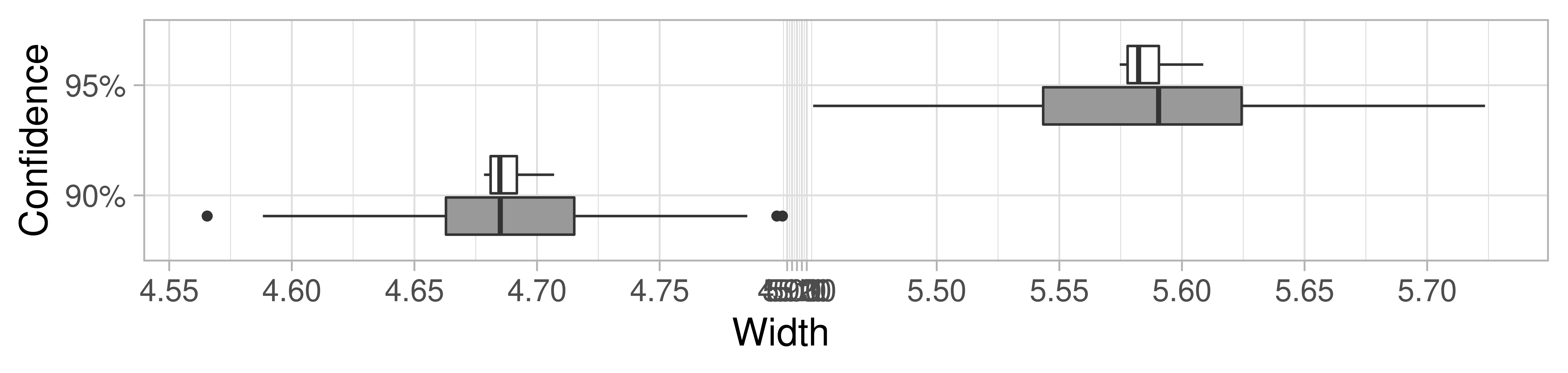
Next, we study the performance and the widths of the 90% and 95% Z-PIs and MC-PIs described in Section 3. To that end, we randomly split the entire data into a training set of size under the constraint that the MAF of each marker is at least 1.5% and a testing set of size We also remove any duplicated markers from the training set, which results in a smaller . We generate 10,000 samples from the approximate posterior predictive distribution (13) to compute the MC-PIs. We find that the Z-PIs and the MC-PIs attain identical coverage rates and these are found to be 91% and 95% for the 90% and 95% prediction intervals, respectively. The boxplots of the widths of the 200 intervals from each method are presented in Figure 3. We find that widths of the the Z-PIs are less variable compared to the same for the MC-PIs. It is encouraging to see that despite non-normality of the posterior prediction distribution, the Z-PIs are better than simulation based intervals.
6 Conclusion
In this article, we introduce a Bayesian variable selection method with embedded screening for ultrahigh-dimensional settings. The model used here is a hierarchical model with well known spike and slab priors on the regression coefficients. Use of the degenerate spike prior for inactive variables not only results in sparse estimates of regression coefficients and (much) lesser computational burden, it also allows us to establish strong model selection consistency under somewhat weaker conditions than Narisetty and He 2014. In particular, we prove that the posterior probability of the true model converges to one even when the norm of mean effects solely due to the unimportant variables diverge. On the other hand, our method crucially hinges on the fact that model probabilities are available in closed form (up to a normalizing constant) which is due to the use of Gaussian slab priors on active covariates. We propose a scalable variable selection algorithm with an inbuilt screening method that efficiently explores the huge model space and rapidly finds the MAP model. The screening is actually model based in the sense that it is performed on a set of candidate models rather than the set of potential variables. The algorithm also incorporates the temperature control into a neighbor based stochastic search method. We use fast Cholesky update to efficiently compute the (unnormalized) posterior probabilities of the neighboring models. Since mean and variance of the posterior predictive distribution are shown to be means of analytically available functions of the models, a derivative of the proposed method is construction of novel prediction intervals for future observations. Both Z based intervals and simulation based intervals are derived and compared. In the context of the real data analysis, we observe that Z based prediction intervals lead to the same coverage rates, although are narrower than Monte Carlo intervals. The extensive simulations studies in section 4 and the real data analysis in section 5 demonstrate the superiority of the proposed method compared with the other state of the art methods, even though the hyperparameters in the proposed method are not carefully tuned. Among the Bayesian methods used for comparison, the package associated with the proposed algorithm seems to be the only one that can be directly applied to datasets of dimension as high as the one analyzed here with the computing resources mentioned before.
Based on the Cholesky update described in Section 2.2.2, SVEN can be extended to accommodate the determinantal point process prior (Kojima and Komaki 2016) on given by where Variable selection and consistency of the resulting posteriors for high dimensional generalized linear models are considered in Liang et al. 2013. It would be interesting to extend our method to the generalized linear regression model setup. The dataset we have used comes from an agricultural field trial and hence the observations are expected to be spatially autocorrelated. Although we have used a two stage procedure by first obtaining spatially adjusted genotypic effects, our model can be extended to include spatial random effects (Dutta and Mondal 2014). Also, in many applications, the covariates may have a non-linear effect on the response and our method could be extended to additive models.
Supplemental materials
The supplemental materials contain additional details on computations and proofs of the theoretical results stated in the paper.
References
- Barbieri and Berger (2004) Barbieri, M. M. and Berger, J. O. (2004), “Optimal predictive model selection,” The Annals of Statistics, 32, 870–897.
- Bertsimas et al. (2016) Bertsimas, D., King, A., and Mazumder, R. (2016), “Best subset selection via a modern optimization lens,” The Annals of Statistics, 44, 813–852.
- Bondell and Reich (2008) Bondell, H. and Reich, B. (2008), “Simultaneous regression shrinkage, variable selection, and supervised clustering of predictors with oscar,” Biometrics, 64, 115–123.
- Cao et al. (2020) Cao, X., Khare, K., and Ghosh, M. (2020), “High-dimensional posterior consistency for hierarchical non-local priors in regression,” Bayesian Analysis, 15, 241–262.
- Chen and Chen (2008) Chen, J. and Chen, Z. (2008), “Extended Bayesian information criteria for model selection with large model spaces,” Biometrika, 95, 759–771.
- Cook et al. (2012) Cook, J. P., McMullen, M. D., Holland, J. B., Tian, F., Bradbury, P., Ross-Ibarra, J., Buckler, E. S., and Flint-Garcia, S. A. (2012), “Genetic architecture of maize kernel composition in the nested association mapping and inbred association panels,” Plant Physiology, 158, 824–834.
- Datta and Zou (2017) Datta, A. and Zou, H. (2017), “Cocolasso for high-dimensional error-in-variables regression,” The Annals of Statistics, 45, 2400–2426.
- Dutta and Mondal (2014) Dutta, S. and Mondal, D. (2014), “An h-likelihood method for spatial mixed linear model based on intrinsic autoregressions,” Journal of the Royal Statistical Society: Series B (Statistical Methodology), 77, 699–726.
- Fan and Li (2001) Fan, J. and Li, R. (2001), “Variable selection via nonconcave penalized likelihood and its oracle properties,” Journal of the American statistical Association, 96, 1348–1360.
- Fan and Lv (2008) Fan, J. and Lv, J. (2008), “Sure independence screening for ultrahigh dimensional feature space,” Journal of the Royal Statistical Society, Series B, 70, 849–911.
- Flint-Garcia et al. (2005) Flint-Garcia, S. A., Thuillet, A.-C., Yu, J., Pressoir, G., Romero, S. M., Mitchell, S. E., Doebley, J., Kresovich, S., Goodman, M. M., and Buckler, E. S. (2005), “Maize association population: a high-resolution platform for quantitative trait locus dissection,” The Plant Journal, 44, 1054–1064.
- George and McCulloch (1993) George, E. I. and McCulloch, R. E. (1993), “Variable selection via Gibbs sampling,” Journal of the American Statistical Association, 88, 881–889.
- George and McCulloch (1997) — (1997), “Approaches for Bayesian variable selection,” Statistica Sinica, 339–373.
- Hans et al. (2007) Hans, C., Dobra, A., and West, M. (2007), “Shotgun stochastic search for “large p” regression,” Journal of the American Statistical Association, 102, 507–516.
- Huang et al. (2018) Huang, J., Jiao, Y., Liu, Y., and Lu, X. (2018), “A constructive approach to L0 penalized regression,” The Journal of Machine Learning Research, 19, 403–439.
- Ishwaran and Rao (2005) Ishwaran, H. and Rao, J. S. (2005), “Spike and slab variable selection: frequentist and Bayesian strategies,” The Annals of Statistics, 33, 730–773.
- Johnson and Rossell (2012) Johnson, V. E. and Rossell, D. (2012), “Bayesian model selection in high-dimensional settings,” Journal of the American Statistical Association, 107, 649–660.
- Kim et al. (2008) Kim, Y., Choi, H., and Oh, H.-S. (2008), “Smoothly clipped absolute deviation on high dimensions,” Journal of the American Statistical Association, 103, 1665–1673.
- Kim et al. (2012) Kim, Y., Kwon, S., and Choi, H. (2012), “Consistent model selection criteria on high dimensions,” Journal of Machine Learning Research, 13, 1037–1057.
- Kirkpatrick et al. (1983) Kirkpatrick, S., Gelatt, C. D., and Vecchi, M. P. (1983), “Optimization by simulated annealing,” science, 220, 671–680.
- Kojima and Komaki (2016) Kojima, M. and Komaki, F. (2016), “Determinantal point process priors for Bayesian variable selection in linear regression,” Statistica Sinica, 26, 97–117.
- Kyung et al. (2010) Kyung, M., Gill, J., Ghosh, M., and Casella, G. (2010), “Penalized Regression, Standard Errors, and Bayesian Lassos,” Bayesian Analysis, 5, 369–412.
- Laurent and Massart (2000) Laurent, B. and Massart, P. (2000), “Adaptive estimation of a quadratic functional by model selection,” Annals of Statistics, 1302–1338.
- Liang et al. (2008) Liang, F., Paulo, R., Molina, G., Clyde, M. A., and Berger, J. O. (2008), “Mixtures of priors for Bayesian variable selection,” Journal of the American Statistical Association, 103, 410–423.
- Liang et al. (2013) Liang, F., Song, Q., and Yu, K. (2013), “Bayesian subset modeling for high-dimensional generalized linear models,” Journal of the American Statistical Association, 108, 589–606.
- Meinshausen and Bühlmann (2006) Meinshausen, N. and Bühlmann, P. (2006), “High-dimensional graphs and variable selection with the lasso,” The Annals of Statistics, 34, 1436–1462.
- Mitchell and Beauchamp (1988) Mitchell, T. J. and Beauchamp, J. J. (1988), “Bayesian variable selection in linear regression,” Journal of the American Statistical Association, 83, 1023–1032.
- Narisetty and He (2014) Narisetty, N. N. and He, X. (2014), “Bayesian variable selection with shrinking and diffusing priors,” The Annals of Statistics, 42, 789–817.
- Park and Casella (2008) Park, T. and Casella, G. (2008), “The Bayesian Lasso,” Journal of the American Statistical Association, 103, 681–686.
- Ročková and George (2014) Ročková, V. and George, E. I. (2014), “EMVS: The EM approach to Bayesian variable selection,” Journal of the American Statistical Association, 109, 828–846.
- Roy and Chakraborty (2017) Roy, V. and Chakraborty, S. (2017), “Selection of tuning parameters, solution paths and standard errors for Bayesian lassos,” Bayesian Analysis, 12, 753–778.
- Roy et al. (2018) Roy, V., Tan, A., and Flegal, J. (2018), “Estimating standard errors for importance sampling estimators with multiple Markov chains,” Statistica Sinica, 28, 1079–1101.
- Shin et al. (2018) Shin, M., Bhattacharya, A., and Johnson, V. E. (2018), “Scalable Bayesian variable selection using nonlocal prior densities in ultrahigh-dimensional settings,” Statistica Sinica, 28, 1053.
- Tibshirani (1996) Tibshirani, R. (1996), “Regression shrinkage and selection via the lasso,” Journal of the Royal Statistical Society: Series B (Methodological), 58, 267–288.
- Wang (2009) Wang, H. (2009), “Forward regression for ultra-high dimensional variable screening,” Journal of the American Statistical Association, 104, 1512–1524.
- Wang and Leng (2016) Wang, X. and Leng, C. (2016), “High dimensional ordinary least squares projection for screening variables,” Journal of the Royal Statistical Society: Series B (Statistical Methodology), 78, 589–611.
- Xu and Ghosh (2015) Xu, X. and Ghosh, M. (2015), “Bayesian variable selection and estimation for group lasso,” Bayesian Analysis, 10, 909–936.
- Yang et al. (2016) Yang, Y., Wainwright, M. J., and Jordan, M. I. (2016), “On the computational complexity of high-dimensional Bayesian variable selection,” The Annals of Statistics, 44, 2497–2532.
- Yuan and Lin (2005) Yuan, M. and Lin, Y. (2005), “Efficient empirical Bayes variable selection and estimation in linear models,” Journal of the American Statistical Association, 100, 1215–1225.
- Zanella and Roberts (2019) Zanella, G. and Roberts, G. (2019), “Scalable importance tempering and Bayesian variable selection,” Journal of the Royal Statistical Society, Series B, 81, 489–517.
- Zellner (1986) Zellner, A. (1986), “On assessing prior distributions and Bayesian regression analysis with g-prior distributions,” in Bayesian inference and decision techniques: Essays in Honor of Bruno de Finetti, eds. Goel, P. K. and Zellner, A., Elsevier Science, 233–243.
- Zhou and Guan (2019) Zhou, Q. and Guan, Y. (2019), “Fast model-fitting of Bayesian variable selection regression using the iterative complex factorization algorithm,” Bayesian analysis, 14, 573.
- Zou (2006) Zou, H. (2006), “The adaptive lasso and its oracle properties,” Journal of the American statistical association, 101, 1418–1429.
- Zou and Hastie (2005) Zou, H. and Hastie, T. (2005), “Regularization and variable selection via the elastic net,” Journal of the royal statistical society: series B (statistical methodology), 67, 301–320.
Supplement to
“Model Based Screening Embedded Bayesian Variable Selection for Ultra-high Dimensional Settings”
Dongjin Li, Somak Dutta and Vivekananda Roy
S1 Efficient computations for multiple predictions
We describe in this section how we efficiently generate multiple in order to obtain the empirical posterior predictive distribution and compute the Monte Carlo prediction intervals at several new covariates . Recall from Section 2.2.2 that for a model , is the upper triangular Cholesky factor of and The detailed procedure is described below.
S2 Comparison of computation time
We examine the computation time it takes for SVEN to hit the MAP model for the first time, and compare it with S5 under the piMOM and the peMOM priors. We simulate the data according to Section 4.1.3, where has an AR(1) structure. We consider five different pairs with where For each of the pair, we obtain the computation times over 10 replicates. For SVEN, we use , and with the temperature schedule described in Section 2.2.2 with Again, S5 is implemented using R-package BayesS5 using their default tuning parameter with only one repetition.
Figure S1 shows the median computation times SVEN and S5 take to first hit the MAP model, excluding the preprocessing steps which are negligible. Both algorithms attain the same MAP model for all the data sets. In general, SVEN hits the MAP model faster than S5 for both small and large number of variables. Moreover, compared to S5, the computation time for SVEN increases at a slower rate as gets larger.
S3 Preliminary results
Let which is the residual sum of squares obtained by ordinary least squares and also let . Before proving the model selection consistency stated in Theorems 1 and 2, we first provide some preliminary results on the bound of which will be used to bound the posterior ratio of a given model to the true model , and the bound of the difference between and .
Lemma 1.
For any model , where is a constant.
Proof.
Because nonzero eigenvalues of and are identical, it follows that . We first show that There are two cases depending on or
Case 1: Suppose We then have
Next, using Sherman–Morrison–Woodbury matrix identity we have,
Thus by letting and we have
| (S1) |
However, note that is the Schuar complement in
so that the smallest eigenvalue of is at least the smallest eigenvalue of which is, in turn, at least because can be obtained by applying one permutation on the rows and columns of Consequently, from (S1), we finally have
because
Case 2: If write where and are disjoint, and Then and
Since , implying . Also, Hence,
Furthermore,
for some where the second to last inequality holds because and the last inequality holds since the condition C3 is in force and the fact that is a submatrix of Since is full rank, . Thus finally we have,
∎
Then, using Lemma 1, we have the following corollary.
Corollary 1.
For any model ,
where , and is a constant.
Lemma 2.
For any sequence , we have
for some .
Proof.
Since and , Sherman–Morrison–Woodbury identity implies
where has rank and by condition C5 has bounded eigenvalues. We want to show that . Next, since , we have
To find the bound of the tail probability, we spilt our proof into following five steps:
- (i)
First, we want to show that . It is clear that
and for some constant . By condition C5 we also know that is bounded. Then with from condition C3, we have for some constant .
- (ii)
Next we will show that . Condition C3 and the fact that has bounded eigenvalues implies that
- (iii)
Next, we will show that for all and and for some , where is distributed as with degrees of freedom. To that end, let , where is an orthogonal matrix and is the diagonal matrix of the eigenvalues of . Then, since , where . Since eigenvalues of are bounded, for some for all . Hence, .
- (iv)
Next we want to show for all , and for some where is distributed as with degrees of freedom. To that end, note that by Cauchy-Schwarz inequality,
However, as in step (iii) above, is stochastically dominated by a constant multiple of distributed random variable since has rank and bounded eigenvalues. Hence by Condition C3, there exists such that
- (v)
Thus all sufficiently large , we have
Now note that , where
is bounded. Also note that
and for sufficiently large Thus, for sufficiently large we have,
for some positive constants and, .
∎
S4 Proof of Theorem 1
To prove the model selection consistency, we use the same strategy as in Narisetty and He 2014 by dividing the set of models into the following subsets:
- (i)
Unrealistically large models: , the models of rank greater than . Abusing notation we use and interchangeably.
- (ii)
Over-fitted models: , the models of rank smaller than which include all the important variables and at least one unimportant variables.
- (iii)
Large models: , that is, the models which miss one or more important variables with rank greater than but smaller than for some fixed positive integer .
- (iv)
Under-fitted models: , the models which have rank smaller than and miss at least one important variable.
We aim to show that for each , with known.
S4.1 Unrealistically large models
We first want to prove that the sum of posterior ratios over converges exponentially to zero. Note that is empty if . The reason is that if , then and , which contradicts the definition of . First, we want to find a set of events that are almost unlikely to happen. So, note that for any ,
| (S2) |
for some , due to Lemma A.2 of Narisetty and He 2014.
Now we consider the term . Condition C2 indicates that because is the smallest eigenvalue of a correlation matrix, i.e., and condition C4 implies that , that is,
| (S3) |
Then we restrict our attention to the high probability event for . Note that, in this case, the upper bound (S4.1) of the probability of the complement of this event is bounded by for some First, by Lemma 1, we have
because for all , , and condition C4 is in force. Recall that . Thus, . Also, by condition C1, for some . Then, due to condition C4 since , we have
as for some , if satisfies , i.e., . Therefore, we have
| (S4) |
S4.2 Over-fitted models
Models in include all important variables plus one or more unimportant variables. For ,
Due to Lemma 1 of Laurent and Massart 2000 and the fact that , for any and for some , we have for all sufficiently large ,
| (S5) | ||||
where and is a constant such that
Now, consider and define the event
Then, for a fixed dimension , consider the event . Since , we have
for some , where the fifth and the sixth inequality hold due to (S5), Lemma 2, condition C2, and the fact that the event depends only on the projection matrix , so we can write the union as a smaller set of events indexed by . Note that since there exists at most subspaces of rank , the cardinality of such projections is at most . Next, we consider the union of all such events , that is,
Note that, as for . Then again restricting to the high probability event , by Lemma 1, (S3) and the fact that is empty, we have
as , where . In the above, we used the fact that and . Note that, since . Hence, we have
| (S6) |
S4.3 Large Models
For models in where the rank is at least and one or more important variables are not inclued, similar to what we’ve shown in Section S4.2, for we use the event
Then we consider the union of such events , for , and . Using (S5) with the fact that and Lemma 2 we have
for some .
Then,
Now, we restrict our attention to the high probability event , we have
as . In the above, we used the fact that by condition C4. Note that because and .
Thus, we have
| (S7) |
S4.4 Under-fitted Models
First, we will prove that for
where is defined in Condition C4. Since , by conditions C3 and C4 we have
for all large . Since , for any , we have
| (S8) |
for some constant . We also have for any ,
for some constant . To see this, let be the SVD of , where . Then, is the projection matrix onto the column space of and thus, using and equation (4) in the main paper, we have
| (S9) |
where the last inequality holds because .
Since the rank of is at most , by (S4.4) and (S3) we have
| (S10) |
The last inequality above holds because by condition C4
Then with , from (S4.4) and (S4.4), we have for any ,
| (S11) |
for some constant . Due to (S4.4) and Lemma 2 with condition C2, for , we have
for some constant . Therefore, restricting to the high probability event
, by corollary 1 and (S3) we get
| (S12) |
because and due to condition C2 and condition C4. Then by (S4.4) we have
| (S13) | ||||
where and To see the last inequality, we consider two cases. First, if and , and thus Then, if . Then, and Therefore, Also, the last line of (S13) holds because by condition C4, , that is, . Hence, we have
| (S14) |
Now, combining (S4), (S6), (S7) and (S14) we get which proves Theorem 1.
S5 Proof of Theorem 2
Next, we will show that with a prior on in (2c), the model selection consistency holds under the assumption that Note that since and , we have eventually. Thus for all large . Therefore, we shall show that for where and . By (2d) and (3) of the main paper, we have
By condition C2 and Lemma 1, we then get
| (S15) |
Define
Due to our Lemma 2 and Lemma A.2(ii) of Narisetty and He 2014, for , we have
| (S16) | ||||
for some positive quantity depending on . From (S15) we have
| (S17) |
Define Note that for models in , . Since condition C6 is in force, we have , and choose and such that and
which is possible since Consequently,
| (S18) |
where the first inequality follows from the fact that for Using the similar way as in Section S4.2, we only consider the high probability event , where is defined the same as in Section S4.2. Note that on , . Note that on , is empty. Then, due to (S17), (S18), and (S3) we obtain