Quasar Sightline and Galaxy Evolution (QSAGE) survey - II. Galaxy overdensities around UV luminous quasars at 2019Quasar Sightline and Galaxy Evolution (QSAGE) survey - II. Galaxy overdensities around UV luminous quasars at –16
Abstract
We demonstrate that the UV brightest quasars at live in overdense environments. This is based on an analysis of deep Hubble Space Telescope WFC3 G141 grism spectroscopy of the galaxies along the lines-of-sight to UV luminous quasars in the redshift range . This constitutes some of the deepest grism spectroscopy performed by WFC3, with 4 roll angles spread over a year of observations to mitigate the effect of overlapping spectra. Of the 12 quasar fields studied, 8 display evidence for a galaxy overdensity at the redshift of the quasar. One of the overdensities, PG0117+213 at , has potentially 36 spectroscopically confirmed members, consisting of 19 with secure redshifts and 17 with single-line redshifts, within a cylinder of radius kpc. Its halo mass is estimated to be . This demonstrates that spectroscopic and narrow-band observations around distant UV bright quasars may be an excellent route for discovering protoclusters. Our findings agree with previous hints from statistical observations of the quasar population and theoretical works, as feedback regulated black hole growth predicts a correlation between quasar luminosity and halo mass. We also present the high signal-to-noise rest-frame optical spectral and photometric properties of the quasars themselves.
Keywords:
quasars: general – galaxies: clusters: general – galaxies: distances and redshifts1 Introduction
Detecting galaxy clusters and protoclusters beyond is challenging but important, as such overdensities are probes of both the accelerated galaxy evolution in dense environments and can provide constraints on cosmological parameters. Modern cluster cosmology generally achieves this via studies of cluster counts (e.g. Vikhlinin et al. 2009; Mantz et al. 2010; de Haan et al. 2016) or the mass fraction of the intracluster medium (ICM) in the most massive systems (e.g. Allen et al. 2008; Ettori et al. 2009; Mantz et al. 2014). The dominant conventional methods for detecting clusters at are via the X-ray emission of the hot ICM (e.g. Ebeling et al. 1998; Böhringer et al. 2004; Finoguenov et al. 2007; Mehrtens et al. 2012), the Sunyaev-Zel’dovich (SZ) effect (Sunyaev & Zeldovich 1972) due to the scattering of cosmic microwave background photons by the ICM (e.g. Staniszewski et al. 2009; Vanderlinde et al. 2010; Planck Collaboration et al. 2014; Bleem et al. 2015; Hilton et al. 2018), and searching for overdensities of passive red galaxies in photometric data (e.g. Gladders & Yee 2005; Koester et al. 2007; Rykoff et al. 2014; Chan & Stott 2019). The flux limited nature of X-ray surveys means it is difficult to find all but the most massive clusters at in significant numbers and in the protocluster phase there may not yet be a mature ICM to provide significant emission. The SZ effect, being a spectral distortion of the microwave background, is in principle redshift independent but still relies on the presence of a mature ICM for the signal so is again not the right tool for selecting less evolved systems. The problem with selecting clusters via overdensities of red galaxies at , is that cluster galaxies are likely to be building up their mass through star formation and are therefore no longer homogenous in colour (Hilton et al. 2010; Tran et al. 2010).
One technique for discovering clusters and protoclusters at , is to search for galaxy overdensities around radio galaxies, which are often the most massive galaxies for their epoch and are therefore likely to live in a clustered environment (e.g. Le Fevre et al. 1996; Best et al. 1998; Pentericci et al. 2000; Kurk et al. 2004; Venemans et al. 2007; Hatch et al. 2011; Wylezalek et al. 2013; Castignani et al. 2014; Husband et al. 2016). This provides a connection and potential evolutionary link to the brightest cluster galaxies (BCGs) found in the low redshift Universe, which are the most massive galaxies and often radio-loud active galactic nuclei (AGN) themselves (e.g. Best et al. 2007; Stott et al. 2012). However, it is important to note that not all distant radio galaxies are found in clustered environments (Hatch et al. 2011; Wylezalek et al. 2013).
In terms of quasars, Wylezalek et al. 2013 find that the majority (55%) of their radio-loud galaxies were in overdensities and there was no significant difference between the environments of radio-loud galaxies or radio-loud quasars. However, radio-quiet AGN such as optical, infrared or X-ray selected quasars are typically found in lower mass galaxies and in less clustered environments, with typical halo masses M⊙ (Kauffmann et al. 2008; Hickox et al. 2009; Ross et al. 2009; Shen et al. 2009; Geach et al. 2019). The environmental difference between radio-loud and radio-quiet AGN may be explained by ‘jet confinement’, in which the denser intergalactic/intracluster medium found in overdensities enhances radiation losses making the radio jets brighter (Barthel & Arnaud 1996). In this case an AGN is more likely to present as radio-loud if in a dense environment. Because of the comparatively low halo masses of optically selected quasars, protocluster searches are usually conducted around radio galaxies instead. However, there are some radio-quiet quasars in dense environments (e.g. Haines et al. 2001) and there has been some success in finding overdensities using pairs of quasars as tracers (Boris et al. 2007).
While it appears that in general, optically selected quasars live in lower density environments than radio galaxies, there is some evidence that the most optically luminous reside in more massive dark matter halos. In their statistical study of halo mass based on the gravitational deflection of the cosmic microwave background, Geach et al. 2019 find that the average halo mass of an optically selected quasar is but those with an absolute band magnitude are in haloes. This is in agreement with the clustering observations of Shen et al. 2009, who find that the 10% most optically luminous quasars are more strongly clustered. However, there is also observational evidence that UV luminous quasars do not live in high mass halos. For example, a galaxy-quasar cross-correlation analysis of a sample of ‘hyperluminous’ quasars at , concludes that they live in modest haloes (Trainor & Steidel 2012). In addition to this, no correlation is found between the locations of bright quasars and a catalogue of overdensities at (Uchiyama et al. 2018).
Despite the uncertain observational picture presented above, there is a theoretical expectation that the UV brightest quasars should live in more massive dark matter halos, as the feedback regulated growth of black holes should result in a relation between black hole mass and halo mass e.g. (Silk & Rees 1998; Wyithe & Loeb 2003). Assuming quasars accrete at an approximately fixed fraction fraction of the Eddingtion limit on average, then the quasar luminosity . Correlations between and are indeed seen in hydrodynamic cosmological simulations of galaxy evolution that employ black hole feedback (Booth & Schaye 2010; McAlpine et al. 2017). One can also think of this as a consequence of the stellar mass – halo mass relation (e.g. Conroy & Wechsler 2009) and the black hole mass – galaxy mass relation (e.g. Magorrian et al. 1998; Ferrarese & Merritt 2000; Gebhardt et al. 2000).
In this paper we test whether UV/optically luminous quasars do indeed trace high density environments using data from the Quasar Sightline And Galaxy Evolution (QSAGE) survey. The QSAGE survey (Bielby et al. 2019) was designed to perform deep Hubble Space Telescope (HST) Wide-Field Camera 3 (WFC3) grism observations centred on 12 quasars with existing high-quality HST UV spectra from the Space Telescope Imaging Spectrograph (STIS) and the Cosmic Origins Spectrograph (COS). The primary purpose of QSAGE is to obtain hundreds of galaxy redshifts in order to associate absorption features in the UV spectra with their host galaxies’ circum-galactic medium (CGM). This information is being used to constrain models of galaxy fuelling and feedback (e.g. Bielby et al. 2017; Bielby et al. 2019).
The paper begins in §2 with a description of the QSAGE sample and data reduction, including the spectral and photometric properties of galaxies and the quasars themselves. In §3 we present the overdensity analysis and results, and look for dependencies between environment and both quasar and galaxy properties. Our findings are discussed in §4 and conclusions drawn in §5.
We adopt a cosmology with = 0.7, = 0.3, and H0 = 70 km s-1 Mpc-1. All quoted magnitudes are on the AB system and we use a Chabrier 2003 IMF throughout.
2 Sample and Data
2.1 WFC3 Data Reduction
The QSAGE survey targets 12 quasars that have existing high quality UV spectra, with the aim of obtaining the redshifts and properties of the galaxy populations along their lines-of-sight (HST Cycle 24 Large Program 14594; PIs: R. Bielby, J. P. Stott). The primary purpose of QSAGE is to perform CGM studies in the redshift range but there is a wealth of additional galaxy evolution science that can be done with the data. The full survey consists of 96 orbits with WFC3 in imaging and grism mode (i.e., 8 orbits per quasar sightline). A detailed description of the spectral and imaging data and its reduction is provided in Bielby et al. 2019, however we briefly describe the key points here.
The HST observations for an individual quasar field consist of 8 grism exposures and supporting near-infrared (NIR) imaging, in order to identify the coordinates of the sources in the grism data. The observations for an individual field are divided into four visits spread out over the year-long HST cycle in order to ensure that each visit is at a different roll angle. This is key because the depth of the grism data requires multiple roll angles to minimise the contamination from the overlapping spectra of neighbouring sources. A visit comprises two orbits, with each orbit scheduled to acquire the following: a single s F140W image; 2 G141 grism exposures of s; and a single s F160W image. In practice, the exposure times were tweaked to optimally fill a given orbit.
The imaging and grism data were reduced using the Grizli software package (Brammer, in prep.11 1 https://github.com/gbrammer/grizli), which is designed for the reduction and analysis of slitless spectroscopic datasets. Grizli builds on the previous aXe (Kümmel et al. 2009) and threedhst (Brammer et al. 2012; Momcheva et al. 2016) software. The F140W and F160W imaging was reduced using TweakReg and then AstroDrizzle. The individual images of a field were combined in a median stack using SWarp (Bertin et al. 2002). The photometric zeropoints were calculated from the image header information ( and ). The photometric catalogues were produced using SExtractor (Bertin & Arnouts 1996) with the F140W catalogue used as the input source coordinates for the G141 grism data.
The approximate 50% completeness values of the F140W and F160W observations are 26.3 mag and 26.1 mag respectively (SExtractor ). These limits are calculated by fitting a straight line to the logarithmic number counts of the magnitude distribution up to its peak then extrapolating this fit beyond the peak and comparing it with the observed number counts (see Fig. 13). The F140W magnitude distribution for the QSAGE sources is presented in Fig. 1.
The F140W catalogues and segmentation images generated by SExtractor were used to extract the spectrum of each object with Grizli. Each of the G141 exposures is first divided by the F140W flat field. An initial background was then subtracted using the ‘master sky’ images from Brammer et al. 2015. These master sky images account for the variation in background structure due to variations in zodiacal continuum, scattered light, and He emission across the sky (Momcheva et al. 2016). The residuals (typically of the initial background levels) were then removed by subtracting average values of the sky pixels in each column. Finally 1D and 2D spectra were extracted from the background-subtracted grism images at the individual exposure level, which, for the QSAGE observations, resulted in 16 individual spectra per object (i.e. 2 spectra per orbit). The advantage of having individual spectra spread out over 4 visits at different times in the HST cycle is that they were taken at four different roll angles. This substantially mitigates the spectral contamination due to neighbouring sources. The contamination for each individual spectrum was calculated using Grizli, which was used to mask heavily contaminated pixels when generating the final stacked spectrum for each source. To aid with visual inspection of the spectra (see §2.2; Fig. 3 of Bielby et al. 2019), a stack was created for each of the four visits (roll angles).

2.2 Spectral fitting
Grism spectra were extracted for a total of 13223 objects across the 12 QSAGE fields. The first step in our analysis was to estimate the emission line redshifts of the galaxies by allowing multiple Gaussians to be fit (with all parameters free, including wavelength) to each spectrum by randomly placing 10 of them throughout the wavelength range in order to search for emission line candidates. This was done iteratively with the first fitted line subtracted from the data before the next fit is attempted, to ensure subsequent fits found different lines. The wavelength range of the WFC3 G141 grism runs from approximately 1075 nm to 1700 nm. The prominent lines and their in-vacuo wavelengths seen in the spectra of star-forming galaxies and AGN in the rest-frame optical range are: [OII] (372.709 nm, 372.988 nm); [OIII] (496.030 nm, 500.824 nm); and H (656.461 nm). The weaker lines that are often still bright enough to easily detect are H (486.272 nm) and [SII] (671.829 nm, 673.268 nm). An estimated redshift solution was found by taking the wavelength ratios of significant () Gaussian fits to determine whether they corresponded to the wavelength ratios of or . At this stage multiple redshift solutions were allowed for each galaxy. All K spectra were then visually inspected alongside the spectra and contaminations for each of the 4 visits (roll angles), and a postage stamp F140W image of the galaxy. This was to either choose the correct redshift solution, provide a new one based on this visual inspection or dismiss the source as a poor solution/spectrum. During this process the spectra were also given a quality flag from with 1 being a poor quality noise-dominated spectra, 2 being low signal-to-noise spectra but with potential spectral lines (), 3 being good quality spectra (lines with ) that are suitable for redshift calculations and 4 being those with higher signal-to-noise (). At this point low- absorption line galaxies, stars, artefacts and potentially interesting objects such as candidate high redshift galaxies and cool brown dwarfs were also categorised.
For the redshift and emission-line analysis in the remainder of the paper we only consider quality 3 and 4 galaxy spectra (example spectra are presented in Fig. 14). The emission-line fluxes are calculated by fitting Gaussian profiles and a local linear continuum. The low resolution of the WFC3 G141 grism ( at 1400 nm) means that the [OII], [OIII] and [SII] doublets, and H and [NII] are unresolved and blended as single lines. For the [OII] we fit a single Gaussian centred on the mid-point of the doublet (372.849 nm). For the [OIII] doublet and H we fit a triplet of Gaussians, as while the [OIII] doublet lines are blended together, they are marginally resolved to the extent that one can observe a distinct asymmetric shape due to the lower flux of the [OIII] 496.030 nm line compared with the 500.824 nm line. The H line is included in the triplet with the [OIII] lines as the low resolution may lead to blending in the wings of these lines. When fitting we assume a fixed flux ratio in the [OIII] doublet of 2.98 (Storey & Zeippen 2000). Again because of the grism resolution, we fit the H and [SII] lines as a doublet of two Gaussians. The H line is fully blended into a single Gaussian with the adjacent [NII] lines (654.986 nm, 658.527 nm). To attempt to extract the true H flux, we assume that the nebula gas has a solar abundance (, Asplund et al. 2004) and thus assuming the linear relation of Pettini & Pagel 2004, the ratio of [NII] 658.527/H is fixed at 0.379. We note however, that solar metallicity is likely too high for galaxies at (Maiolino et al. 2008). In the absence of individual metallicity information for the galaxies, the effect of this is to potentially underestimate the H flux and therefore star formation rate (SFR) of the sample. If there is a significant difference in metallicity between the overdensity and field, this could potentially affect the comparison of SFR with environment presented in §3.3 . The flux ratio of the redder 658.527 nm is fixed to be 2.95 greater than that of the fainter blue [NII]654.986 nm line, as is the theoretical expectation. The [SII] doublet is completely blended and so we treat it as a single Gaussian centred on the average wavelength of 672.548 nm. To obtain the completeness limit of the spectroscopy, the flux distribution of the Gaussian fits to the blended H and [NII] lines is presented in Fig. 2. This has a median flux of erg s-1 cm-2 and an approximate 50% completeness of erg s-1 cm-2.
The redshifts we can access for the majority of the QSAGE galaxy population are: ([OII]), (H), ([OIII]) and (H). There is therefore, continuous coverage in redshift from . Within this, there are ranges in redshift where the spectroscopic redshift is unambiguous, as multiple bright lines are present within the grism’s wavelength window. These multiple line windows are [OIII] and H at , and [OII] and [OIII] at . Where the, generally weaker, secondary line is visible it is also possible to obtain unambiguous redshifts from H and [OIII] at and H and [SII] at . Finally, in high signal to noise cases, the asymmetry in the blended [OIII] (496.030 nm, 500.824 nm) can also provide an unambiguous redshift from . In cases of single and therefore ambiguous lines we do not assign a redshift, although we show the result of assuming a line identity in §3.1. In total, we obtain good spectra for 1437 galaxies. Of these, 844 have unambiguous redshifts with the remaining 593 being ambiguous single-line detections. For the remainder of the paper, we will refer to the galaxies with unambiguous redshifts as the unambiguous- sample. The distribution of the unambiguous- sample redshifts is plotted in Fig. 3. We note the peak in this graph at , which reflects the ease of obtaining unambiguous redshifts in that window as discussed above. In order to break the single-line degeneracy and produce a more complete set of QSAGE redshifts, spectral energy distribution (SED) fitting will be performed and presented in Bielby et al., in prep.


2.3 Quasar properties
The 12 central quasars of the QSAGE sample are presented with their redshifts, photometry and emission line fluxes in Table 1. All of the quasar spectra with the necessary wavelength coverage also show the presence of H, H, [OI], [NeIII] and the FeII multiplet complexes at Å and Å (see Phillips 1978 and Zhou et al. 2002). Example WFC3 quasar spectra are shown in Fig. 4. A column for [OII] flux is not included in Table 1 as QSO-B1122-168 is the only quasar with this line in its redshift range and despite a very high signal-to-noise spectrum, it is not detected (see Fig. 4). This is likely due to the radiation from the quasar causing a high ionisation state, which means that most of the oxygen emission is via [OIII] instead (although this is out of the wavelength window for this quasar). Any [OII] emission due to star formation in the host is likely to be completely overwhelmed by the continuum emission of the quasar.
QSO-B0810+2554 is a known quadruply lensed quasar (Reimers et al. 2002), which is potentially interesting for cosmology via gravitational lens time delays (e.g. Congdon et al. 2010; Wong et al. 2019). The QSAGE F140W image of this lens is displayed in Fig. 5. We find no evidence for lensing in the remaining QSAGE quasars.
| Quasar | R.A. | Dec. | F140W | F160W | |||||
|---|---|---|---|---|---|---|---|---|---|
| PG0117+213 | 01:20:17.3 | +21:33:46.2 | 1.5041 | 15.5 | 15.8 | 15.6 | 1.690.29 | 0.700.19 | 12.661.03 |
| PKS-0232-04 | 02:35:07.3 | -04:02:05.3 | 1.4428 | 16.3 | 16.3 | 16.1 | 2.510.29 | 1.030.19 | 10.990.44 |
| HE0515-4414 | 05:17:07.6 | -44:10:55.6 | 1.7332 | 15.1 | 14.6 | 14.6 | 4.380.35 | 1.280.24 | … |
| 2QSO-B0747+4259 | 07:50:54.6 | +42:52:19.3 | 1.9151 | 15.6 | 15.5 | 15.5 | 2.780.17 | 0.740.11 | … |
| QSO-B0810+2554 | 08:13:31.3 | +25:45:03.1 | 1.5103 | 15.5 | 15.2 | 14.9 | 5.250.53 | 0.860.32 | 33.451.87 |
| QSO-J1019+2745 | 10:19:56.6 | +27:44:01.7 | 1.9298 | 15.6 | 16.0 | 15.9 | 2.660.16 | 0.990.11 | … |
| QSO-B1122-168 | 11:24:42.9 | -17:05:17.4 | 2.4181 | 16.5 | 16.1 | 16.1 | 2.480.17 | … | … |
| QSO-J1130-1449 | 11:30:07.1 | -14:49:27.4 | 1.1896 | 16.1 | 17.2 | 23.9 | … | … | 5.710.13 |
| LBQS-1435-0134 | 14:37:48.3 | -01:47:10.8 | 1.3061 | 15.1 | 15.3 | 15.1 | 5.420.90 | 3.760.68 | 18.280.55 |
| QSO-B1521+1009 | 15:24:24.5 | +09:58:29.1 | 1.3266 | 14.7 | 15.8 | 15.7 | 4.481.17 | 1.310.75 | 10.430.36 |
| QSO-B1630+3744 | 16:32:01.1 | +37:37:50.0 | 1.4787 | 16.0 | 15.9 | 15.7 | 1.980.27 | 0.540.17 | 10.610.51 |
| QSO-B1634+7037 | 16:34:29.0 | +70:31:32.4 | 1.3319 | 14.9 | 14.3 | 14.1 | 7.901.80 | 8.321.36 | 55.321.75 |


2.4 Star formation rates
The star formation rates of all of the galaxies with redshifts are calculated using the H and [OII] fluxes, which for the former accounts for [NII] contamination assuming solar metallicity as discussed in §2.2. We use the relationships between nebula line flux and star formation from Kennicutt 1998 assuming a correction to a Chabrier 2003 stellar initial mass function (IMF). A constant extinction of is also assumed, which is appropriate to star-forming galaxies in a similar mass range (Sobral et al. 2012). This corresponds to and using the extinction curve of Cardelli et al. 1989. Fig. 6 displays the SFR distribution of the QSAGE galaxies. The median H and [OII] SFRs for the sample are M⊙ yr-1 and M⊙ yr-1 respectively. We note that due to the wavelength range available, no galaxies have a detection of both H and [OII] (see Fig. 3) and so this apparent discrepancy just reflects the fact that the sample detected in [OII] has a higher SFR due to the flux limited nature of the observations. It will be possible to refine the SFR with the and metallicity values calculated via SED fitting in Bielby et al. in prep. That paper will also greatly increase the number of SFR values available by breaking the single-line redshift degeneracy as discussed in §2.2.

2.5 Stellar Masses
The stellar masses of all of the galaxies with redshifts are approximately calibrated using the linear relationship between full SED fit stellar mass and F160W magnitude that we derive in bins of 0.1 in redshift from the Cosmic Assembly Near-infrared Deep Extragalactic Legacy Survey (CANDELS) catalogues of Barro et al. 2019. An example of this relation at (the approximate median redshift of the QSAGE quasars) is shown in Fig. 15. This calibration is appropriate to make for this paper as stellar mass only features in §3.3. The fit parameters we calculate as a function of redshift are given in Table 3. The stellar mass distribution of the QSAGE galaxies based on this approximation is displayed in Fig. 7. The median mass of the sample is . An improved set of stellar mass values will be calculated via full SED fitting in Bielby et al., in prep. That paper will also greatly increase the number of mass values available by breaking the single-line redshift degeneracy.

3 Analysis and Results
3.1 Quasar environments
We search for the presence of overdensities in the redshift distribution in the vicinity of the central QSAGE target quasars. The advantage of using a grism for this analysis is that we obtain an unbiased sample of line-emitting galaxies as there is no preselection of spectroscopic targets. While this is also true for previous narrow-band surveys (e.g., Le Fevre et al. 1996; Kurk et al. 2004; Husband et al. 2016) we are not restricted to only studying quasars at the redshifts in which a narrow-band filter can isolate an emission line. In addition, our unambiguous- sample is unaffected by interlopers due to alternative spectral lines from galaxies at different redshifts being detected in the narrow-band filter. Our method for finding overdensities is to search for an excess in galaxies in a fixed redshift bin centred on the measured WFC3 grism quasar redshift. The choice of reflects a combination in quadrature of the spectral resolution of the grism (instrumental velocity dispersion km s-1) and the typical velocity dispersion of a forming cluster ( km s-1) and a factor of to account for the expansion of the Universe (using the approximate average quasar redshift, ). The individual redshift distributions are presented in Figures 8 and 9.
To assess the environment of the quasars we use the overdensity parameter, , which is given by
| (1) |
where is the number of unambiguous- galaxies in the bin centred on the redshift of the quasar and is the average background i.e. the expected number of galaxies in the absence of any significant structure. The calculation of this background value, , is therefore key to understanding the significance of the galaxy overdensity.
The overdensity parameter is often used when the presence of an excess of galaxies is being assessed with narrow-band imaging (e.g. Husband et al. 2016). In that case, the number of narrow-band selected galaxies at the redshift of the quasar/radio galaxy is compared with the number of galaxies selected in the same narrow-band (to the same magnitude limit) when averaged over a large area or from ‘blank’ fields. In our case, we are searching for potential overdensities at 12 different redshifts in fields in which galaxies in a similar redshift range are detected and selected in the same way. This can be used to our advantage as it means we can generate an average background in redshift space using adjacent redshift bins to the quasar itself in combination with those from the remaining 11 quasar fields.
The average background redshift distribution is generated by averaging all 12 of the galaxy redshift distributions for the different fields together. Specifically, the redshift distributions were placed on a common bin scale of , with the mean number of galaxies calculated for each bin to create the background distribution. The common bin scale required small shifts of as the quasars are fixed at the centre of their redshift bin for a particular field. We do not believe that this small shift will cause any biases in the analysis. The bins containing the quasar in each individual field are also removed from the average in case any particularly significant overdensities contaminate the background of the others. For the background value, , we take the mean value of this averaged background redshift distribution in the bins with from the quasar, with a buffer around the redshift bin of the quasar being excluded from the analysis in order to avoid an inflated background due to self-contamination. The errors on are calculated using the Poisson error on combined in quadrature with the standard error on the background distribution. We note that using the Poisson error means that a galaxy overdensity would need at least 9 members to be considered to have a significance (where is the error on ), which may be somewhat conservative and so we adopt a threshold, following Galametz et al. 2012; Wylezalek et al. 2013. The overdensity values are presented in Table 2. Of the 12 fields studied, 8 contain overdensities, showing that of our quasars are in overdense environments. Our richest galaxy overdensity is PG0117+213 with 19 unambiguous- members and a further 17 potential single-line redshift members, 36 in total (see Fig. 8). The additional 17 potential members are single-line galaxies, which would fall into the quasar’s redshift bin if the line is confirmed to be H. The F140W images of the QSAGE fields, with galaxies in the same redshift bin as the quasars highlighted, are displayed in Fig. 10.
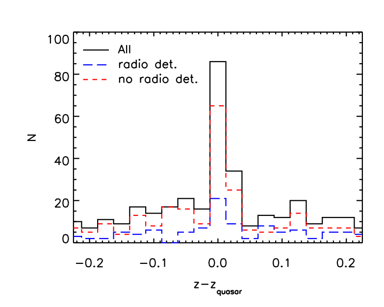
In addition to the overdensities calculated for the individual quasar fields, we also stack the redshift distributions of all 12 fields in such a way that each field that goes into the stack is centred on the redshift bin of the individual quasars. In this way a stacked redshift ‘cluster’ is created and shown in Fig. 11. The overdensity of this stack is , (i.e. a significance of ), clearly demonstrating that, on average, the QSAGE quasars are in overdense environments.
3.1.1 Additional overdensities
We note that there are potentially ( member) overdensities at redshifts not associated with the quasars in the fields: HE0515-4414 (6 members); QSO-B0747+4259 (6 members); QSO-B0810+2554 (6, 6 and 7 members); and QSO-B1630+3744 (9 members). These are not analysed further in this paper.


| field name | Radio | R.A. | Dec. | |||||||
|---|---|---|---|---|---|---|---|---|---|---|
| PG0117+213 | 19 | 17 | 17.5 | 4.8 | 3.6 | n | -28.8 | 01:20:17.5 | +21:33:44.6 | 14.70.5 |
| PKS-0232-04 | 7 | 4 | 6.3 | 2.9 | 2.2 | y | -28.0 | 02:35:08.3 | -04:01:46.4 | 14.30.4 |
| HE0515-4414 | 7 | 1 | 9.7 | 4.4 | 2.2 | n | -29.5 | 05:17:08.8 | -44:10:41.6 | 14.50.4 |
| QSO-B0747+4259 | 2 | 3 | 3.5 | 3.3 | 1.1 | n | -29.3 | 07:50:54.4 | +42:52:19.0 | … |
| QSO-B0810+2554 | 2 | 1 | 1.1 | 1.5 | 0.7 | n | -28.8 | 08:13:30.9 | +25:45:22.9 | … |
| QSO-J1019+2745 | 7 | 3 | 13.9 | 6.1 | 2.3 | n | -29.3 | 10:19:55.6 | +27:43:57.3 | 14.70.4 |
| QSO-B1122-168 | 1 | 0 | … | … | … | y | -28.9 | 11:24:42.9 | -17:05:17.4 | … |
| QSO-J1130-1449 | 2 | 6 | 1.3 | 1.6 | 0.8 | y | -27.7 | 11:30:05.9 | -14:49:42.4 | … |
| LBQS-1435-0134 | 11 | 4 | 9.4 | 3.4 | 2.8 | y | -28.9 | 14:37:47.8 | -01:47:12.5 | 14.40.4 |
| QSO-B1521+1009 | 6 | 1 | 5.3 | 2.7 | 2.0 | n | -29.4 | 15:24:23.8 | +09:58:29.8 | 14.20.4 |
| QSO-B1630+3744 | 13 | 2 | 12.7 | 4.2 | 3.0 | n | -28.3 | 16:32:02.3 | +37:37:49.5 | 14.60.4 |
| QSO-B1634+7037 | 9 | 3 | 8.2 | 3.3 | 2.5 | n | -29.2 | 16:34:31.5 | +0:31:47.1 | 14.40.4 |
| Stack | 86 | 45 | 5.8 | 0.9 | 6.6 |


3.2 Overdensity masses
In this section we attempt to estimate the mass of the overdensities in order to understand what kinds of structures they comprise and what they will become by . We estimate the masses using the galaxy overdensity parameter, , following the method of Venemans et al. 2005 in which the mass, is given by
| (2) |
where is the average density of the Universe at the redshift of the galaxy overdensity; is the comoving volume within which the overdensity is calculated; and is the mass overdensity, which is given by , where is the bias of individual galaxy halos and not the overdensity (see e.g. Steidel et al. 1998). The comoving volumes probed by our observations are calculated individually with a typical value at of Mpc3. These overdensities may not be virialised and so should be interpreted as the total mass that these systems will collapse to become by . To estimate the bias we use the results presented in Cochrane et al. 2017, in which the bias is measured as a function of H luminosity and redshift. Their relation between bias and at is the most appropriate to our sample; however the data are noisy at the faint end and do not probe to low enough luminosities for our observations. We therefore fit a relation to the strong linear trend seen between bias and at and then make the assumption that this slope also applies at . A linear fit is then performed on the relation, with the slope fixed to the value in order to constrain the intercept. This is illustrated in Fig. 16. The mean H luminosity of the galaxies within the overdensities is (erg s-1) and so the bias value we estimate is based on this analysis of the Cochrane et al. 2017 data, which is consistent with the clustering measurements of the QSAGE sample at (Bielby et al., in prep.). The overdensity derived masses are presented in Table 2. The mass errors are based solely on the error on and not the assumed bias parameter, , and so these errors are potentially larger. If the overdensities are not virialised, then these masses can be considered to be the mass that could potentially collapse out from this volume in order to form a single cluster by . The masses derived demonstrate that the mass within each of the 8 significant overdensities is in the range , with an average of . We note that due to the size of the, likely underestimated, error bars on the the individual overdensity masses they are all consistent with each other. However, due to lack of a full census of galaxies within the overdensities and the potentially naive assumption made that all mass within the Mpc3 volume will collapse into one structure by , in reality we expect their final virialised masses to cover a range of values.
3.3 Investigating dependencies
The QSAGE quasars were selected to be luminous in the UV and blue optical to ensure that high signal-to-noise spectra could be obtained for quasar absorption line studies of the intergalactic medium. If quasar luminosity depends on halo mass (e.g. Silk & Rees 1998; Geach et al. 2019) then we may expect to observe such a correlation. Therefore, we take the -band magnitude from the USNO A2 (Monet 1998; see Table 1) and the quasar correction from Wisotzki 2000 to calculate the absolute -band magnitude in the AB system (assuming a conversion from Vega to AB of magnitudes). In Fig. 12 we plot absolute -band magnitude, , against the overdensity parameter, and find no correlation. This suggests that while the brightest quasars are often in overdensities, their luminosities do not increase monotonically with .
As discussed in §1, there has been great success in searching for overdense environments in the vicinity of radio galaxies (e.g. Venemans et al. 2007; Hatch et al. 2011; Wylezalek et al. 2013; Husband et al. 2016). The quasar sample presented here was not selected to be radio emitting, however some are known radio sources and so we look for a connection between the overdensity parameter and presence of a radio counterpart. All of the QSAGE quasars are covered by the all-sky radio surveys: the National Radio Astronomy Observatory (NRAO) Very Large Array (VLA) Sky Survey (NVSS, Condon et al. 1998); the Faint Images of the Radio Sky at Twenty-Centimeters (FIRST, Becker et al. 1995) in the North; and the Sydney University Molonglo Sky Survey (SUMSS, Mauch et al. 2003) in the South. The coordinates of the QSAGE quasars are entirely covered by a combination of these three surveys and are matched to them using the radii recommended for each survey: NVSS (45”); FIRST (30”); and SUMSS (45”). We find that 4 out of the 12 quasars are radio emitters but see no evidence for greater overdensities in these fields, as shown in Table 2 and Figures 11 and 12.
Galaxy clusters and dense environments tend to contain more massive and more passive galaxies than the field population in the local Universe (Dressler 1980; Peng et al. 2010). However, it is expected that at higher redshift there is a reversal of the star formation rate local density relation in order for the constituent galaxies to build up their masses at a faster rate than the field (e.g. Hilton et al. 2010; Tran et al. 2010). We therefore compare the properties of the galaxies within the same redshift bin as the quasar to those within the redshift range (i.e. the approximate redshift range of the quasar sample) to see if higher stellar mass and/or more passive galaxies are already in place in these systems or if they are building up their mass at a greater rate. The median stellar mass of all of the unambiguous galaxies (excluding the quasars) within is and the median mass of those within the same redshift bin as the quasars (again excluding the quasars) is . The median mass of those in the most significant galaxy overdensity, PG0117+213, is . There is therefore no evidence for a difference in mass between the population in the same structure as the quasar and that of the field. However, due to the line-emission selection we may be missing a population of high mass passive galaxies.
The median H derived SFR for the unambiguous galaxies (excluding the quasars) with redshifts (i.e. the redshift range over which we can detect H) is M⊙yr-1 and for those in the same redshift bins as their quasars (again excluding the quasars) it is M⊙yr-1. Therefore, there is no evidence for a difference between the SFR of the galaxies within the overdensities and those in the field. However, as discussed in §2.2, a systematic difference in gas phase metallicity between the field and overdensities could affect this, as we assume a single metallicity for the whole sample to extract H flux from the blended H and [NII] line. Additionally, due to the line-emission selection we may be missing a population of more passive galaxies.

4 Discussion
From the analyses of the redshift distributions of the individual quasar fields, we find that 8/12 of the QSAGE quasars are in overdensities and the combined stack of the redshift distributions confirms this is true on average (see Fig. 11). The overdensities have inferred masses of , indicating that they are either already galaxy clusters or regions of space that will collapse further into galaxy clusters by . The richest galaxy overdensity in our sample is found around the quasar PG0117+213, which has 19 confirmed members and potentially 36 in total and as such, its predicted mass of is likely a lower limit. We note that a narrow-band survey would have determined that all line-emitters within the narrow-band filter wavelength range were potential members. One of the least dense fields is QSO-B0810+2554, which is the lensed quasar discussed in §2.3, there is a possibility that this quasar’s intrinsic brightness has been boosted by the lensing to bring it into the sample. In general, the overdensity values and masses will be lower limits, as we did not include the single-line emitters with ambiguous redshifts and our emission line selection will not have detected the passive galaxies present in clusters.
Overdensities such as these have often been found for radio galaxy fields (e.g. Venemans et al. 2007; Hatch et al. 2011; Wylezalek et al. 2013; Husband et al. 2016) but this has been less clear for those surrounding quasars, which typically reside in dark matter halos (Kauffmann et al. 2008; Hickox et al. 2009; Ross et al. 2009; Shen et al. 2009; Geach et al. 2019). However, as discussed in §1 there are both theoretical arguments and observational hints that the most UV/optically bright quasars live in higher mass halos. The feedback regulated growth of black holes should result in a relation between black hole mass and halo mass e.g. (Silk & Rees 1998; Wyithe & Loeb 2003) and so assuming accretion is approximately at a fixed fraction of the Eddington limit, the quasar luminosity . Statistical studies have attempted to confirm this, finding that the brighter quasars in their clustering analyses reside in higher mass halos (e.g. , Geach et al. 2019). However, results at show no evidence that the brightest quasars live in overdensities (Uchiyama et al. 2018).
Our QSAGE sample includes some of the brightest quasars at , and we have demonstrated, for the first time, that the brightest quasars really are in highly overdense environments. We speculate that the reason this is not seen in lower redshift clusters is that clusters in the local Universe tend to be dominated by passive red sequence galaxies (Dressler 1980; Peng et al. 2010), which contain significantly less cold gas to fuel a quasar. At , there must be a reversal of this relation in order for the cluster galaxies to build up their stellar mass through star formation and so clusters and protoclusters contain more gas rich galaxies at early times (e.g. Hilton et al. 2010; Tran et al. 2010). This combination of a high halo mass, gas-rich environment means that luminous quasars are more likely to be good tracers of cluster and protoclusters rather than their low redshift counterparts. Our results demonstrate that searching for overdensities around the brightest quasars is an excellent way to find high redshift clusters and protoclusters.
The discrepancy between our results and the lack of overdensities found around bright quasars at (Uchiyama et al. 2018), may be due to several factors. Firstly, our redshift range is lower and so perhaps the bright quasar population live in low mass halos at , with little evolutionary connection to their counterparts. Secondly, the Uchiyama et al. 2018 study uses a photometric overdensity catalogue created from -band drop out galaxies, whereas our deep grism data means that we obtain a spectroscopic redshift census of the line-emitting galaxies in the field. It may therefore be the case that we can probe structures that would be missed by a photometric technique.
One potential reason for finding the brightest quasars within overdense environments is that they may be regions of high merger or interaction activity, which will both increase the black hole’s mass through merging and accretion, as gas is disturbed and funnelled towards the black hole. Another related explanation is that these luminous quasars contain the most massive black holes (and therefore have high Eddington luminosities) in the cluster because they are the progenitors of the BCG population, going through a rapid stellar and black hole mass growth phase via mergers and/or accretion (Hlavacek-Larrondo et al. 2013). These scenarios are in agreement with the ‘blowout’ phase of the evolutionary path described by Hopkins et al. 2008.
Within the sample, we find there is no relationship between the luminosity of the quasar and the strength of the overdensity. This may in part be related to the variable nature of quasar luminosity (e.g. MacLeod et al. 2012), which is governed by variability in the fuelling rate, and/or as the observations are rest-frame UV, a small amount of dust obscuration could also act to remove any correlation.
There is no evidence for enhancement of the overdensities around the radio emitting quasars compared with the sample as a whole. This is in apparent contrast to Wylezalek et al. 2013, although only of their sample of radio-loud quasars show such an enhancement and our survey contains only four radio emitters so we do not draw any conclusions from this.
Finally, there is no evidence that the galaxy populations within the overdensities are different to those in the field in terms of stellar mass or SFR. This is further evidence for a reversal of SFR - local density relation at as the overdensity members appear to be forming stars at the same rate as their field counterparts, in contrast to clusters. However, as this sample is selected on line-emission, we may be missing a significant number of massive and passive galaxies.
5 Summary & conclusions
In this paper, we demonstrate that 8/12 of the QSAGE quasars reside in overdensities with masses of . This is strong evidence to support the hypothesis that the brightest quasars should live in the most massive dark matter halos (Silk & Rees 1998; Wyithe & Loeb 2003). It also paves the way for future narrow-band, grism or integrated field spectroscopy studies of the populations around high- quasars in order to look for protoclusters. Of particular note is PG0117+213, which is a rich structure with up to 36 members within a cylinder of kpc radius and . We speculate that the reason we are finding bright quasars within these overdensities is due to a increased mergers activity and/or even the mass build up of a BCG progenitor. The galaxies within the overdensities appear to have similar masses and SFR to those in the field, which is further evidence for a reversal of SFR - local density relation at .
This paper represents part of the galaxy evolution component of the QSAGE survey, which has the primary goal of obtaining hundreds of galaxy redshifts in order to associate absorption features in the UV spectra of quasars with their host galaxies’ CGM. Combined, these two components of the QSAGE survey will provide comprehensive constraints to the galaxy fuelling and feedback process in galaxy formation models.(e.g. Bielby et al. 2019 and forthcoming papers).
Acknowledgements
We first thank the anonymous referee for improving the clarity of the paper. We also thank James Mullaney, Nic Ross and David Sobral for useful discussions. RMB, MF, RGB, and SLM acknowledge the Science and Technology Facilities Council (STFC) through grants ST/P000541/1 and ST/L00075X/1 for support. This project has received funding from the European Research Council (ERC) under the European Union’s Horizon 2020 research and innovation programme (grant agreement No 757535). This work has been supported by Fondazione Cariplo, grant number 2018-2329. JNB and JXP received financial support for this research through NASA Grant HST-GO-11741 from the Space Telescope Science Institute, which is operated by the Association of Universities for Research in Astronomy, Inc., under NASA Contract NAS5-26555. RAC is a Royal Society University Research Fellow.
Data availability
The data underlying this article are from HST Cycle 24 proposal 14594: ‘QSAGE: QSO Sightline And Galaxy Evolution’ and are publicly available from the Mikulski Archive for Space Telescopes (MAST, https://archive.stsci.edu/hst/).
References
- Allen et al. (2008) Allen S. W., Rapetti D. A., Schmidt R. W., Ebeling H., Morris R. G., Fabian A. C., 2008, MNRAS, 383, 879
- Asplund et al. (2004) Asplund M., Grevesse N., Sauval A. J., Allende Prieto C., Kiselman D., 2004, A&A, 417, 751
- Barro et al. (2019) Barro G., et al., 2019, ApJS, 243, 22
- Barthel & Arnaud (1996) Barthel P. D., Arnaud K. A., 1996, MNRAS, 283, L45
- Becker et al. (1995) Becker R. H., White R. L., Helfand D. J., 1995, ApJ, 450, 559
- Bertin & Arnouts (1996) Bertin E., Arnouts S., 1996, A&AS, 117, 393
- Bertin et al. (2002) Bertin E., Mellier Y., Radovich M., Missonnier G., Didelon P., Morin B., 2002, in Bohlender D. A., Durand D., Handley T. H., eds, Astronomical Society of the Pacific Conference Series Vol. 281, Astronomical Data Analysis Software and Systems XI. p. 228
- Best et al. (1998) Best P. N., Longair M. S., Roettgering H. J. A., 1998, MNRAS, 295, 549
- Best et al. (2007) Best P. N., von der Linden A., Kauffmann G., Heckman T. M., Kaiser C. R., 2007, MNRAS, 379, 894
- Bielby et al. (2017) Bielby R., Crighton N. H. M., Fumagalli M., Morris S. L., Stott J. P., Tejos N., Cantalupo S., 2017, MNRAS, 468, 1373
- Bielby et al. (2019) Bielby R. M., et al., 2019, MNRAS, 486, 21
- Bleem et al. (2015) Bleem L. E., et al., 2015, ApJS, 216, 27
- Böhringer et al. (2004) Böhringer H., et al., 2004, A&A, 425, 367
- Booth & Schaye (2010) Booth C. M., Schaye J., 2010, MNRAS, 405, L1
- Boris et al. (2007) Boris N. V., Sodré L. J., Cypriano E. S., Santos W. A., de Oliveira C. M., West M., 2007, ApJ, 666, 747
- Brammer et al. (2012) Brammer G. B., et al., 2012, ApJS, 200, 13
- Brammer et al. (2015) Brammer G., Ryan R., Pirzkal N., 2015, Technical report, Source-dependent master sky images for the WFC3/IR grisms
- Cardelli et al. (1989) Cardelli J. A., Clayton G. C., Mathis J. S., 1989, ApJ, 345, 245
- Castignani et al. (2014) Castignani G., Chiaberge M., Celotti A., Norman C., De Zotti G., 2014, ApJ, 792, 114
- Chabrier (2003) Chabrier G., 2003, PASP, 115, 763
- Chan & Stott (2019) Chan M. C., Stott J. P., 2019, MNRAS, 490, 5770
- Cochrane et al. (2017) Cochrane R. K., Best P. N., Sobral D., Smail I., Wake D. A., Stott J. P., Geach J. E., 2017, MNRAS, 469, 2913
- Condon et al. (1998) Condon J. J., Cotton W. D., Greisen E. W., Yin Q. F., Perley R. A., Taylor G. B., Broderick J. J., 1998, AJ, 115, 1693
- Congdon et al. (2010) Congdon A. B., Keeton C. R., Nordgren C. E., 2010, ApJ, 709, 552
- Conroy & Wechsler (2009) Conroy C., Wechsler R. H., 2009, ApJ, 696, 620
- Dressler (1980) Dressler A., 1980, ApJ, 236, 351
- Ebeling et al. (1998) Ebeling H., Edge A. C., Bohringer H., Allen S. W., Crawford C. S., Fabian A. C., Voges W., Huchra J. P., 1998, MNRAS, 301, 881
- Ettori et al. (2009) Ettori S., Morandi A., Tozzi P., Balestra I., Borgani S., Rosati P., Lovisari L., Terenziani F., 2009, A&A, 501, 61
- Ferrarese & Merritt (2000) Ferrarese L., Merritt D., 2000, ApJ, 539, L9
- Finoguenov et al. (2007) Finoguenov A., et al., 2007, ApJS, 172, 182
- Galametz et al. (2012) Galametz A., et al., 2012, ApJ, 749, 169
- Geach et al. (2019) Geach J. E., Peacock J. A., Myers A. D., Hickox R. C., Burchard M. C., Jones M. L., 2019, ApJ, 874, 85
- Gebhardt et al. (2000) Gebhardt K., et al., 2000, ApJ, 539, L13
- Gladders & Yee (2005) Gladders M. D., Yee H. K. C., 2005, ApJS, 157, 1
- Haines et al. (2001) Haines C. P., Clowes R. G., Campusano L. E., Adamson A. J., 2001, MNRAS, 323, 688
- Hatch et al. (2011) Hatch N. A., et al., 2011, MNRAS, 410, 1537
- Hickox et al. (2009) Hickox R. C., et al., 2009, ApJ, 696, 891
- Hilton et al. (2010) Hilton M., et al., 2010, ApJ, 718, 133
- Hilton et al. (2018) Hilton M., et al., 2018, ApJS, 235, 20
- Hlavacek-Larrondo et al. (2013) Hlavacek-Larrondo J., Fabian A. C., Edge A. C., Ebeling H., Allen S. W., Sanders J. S., Taylor G. B., 2013, MNRAS, 431, 1638
- Hopkins et al. (2008) Hopkins P. F., Hernquist L., Cox T. J., Kereš D., 2008, ApJS, 175, 356
- Husband et al. (2016) Husband K., Bremer M. N., Stott J. P., Murphy D. N. A., 2016, MNRAS, 462, 421
- Kauffmann et al. (2008) Kauffmann G., Heckman T. M., Best P. N., 2008, MNRAS, 384, 953
- Kennicutt (1998) Kennicutt Jr. R. C., 1998, ARA&A, 36, 189
- Koester et al. (2007) Koester B. P., et al., 2007, ApJ, 660, 239
- Kümmel et al. (2009) Kümmel M., Walsh J. R., Pirzkal N., Kuntschner H., Pasquali A., 2009, PASP, 121, 59
- Kurk et al. (2004) Kurk J. D., Pentericci L., Röttgering H. J. A., Miley G. K., 2004, A&A, 428, 793
- Le Fevre et al. (1996) Le Fevre O., Deltorn J. M., Crampton D., Dickinson M., 1996, ApJ, 471, L11
- MacLeod et al. (2012) MacLeod C. L., et al., 2012, ApJ, 753, 106
- Magorrian et al. (1998) Magorrian J., et al., 1998, AJ, 115, 2285
- Maiolino et al. (2008) Maiolino R., et al., 2008, A&A, 488, 463
- Mantz et al. (2010) Mantz A., Allen S. W., Rapetti D., Ebeling H., 2010, MNRAS, 406, 1759
- Mantz et al. (2014) Mantz A. B., Allen S. W., Morris R. G., Rapetti D. A., Applegate D. E., Kelly P. L., von der Linden A., Schmidt R. W., 2014, MNRAS, 440, 2077
- Mauch et al. (2003) Mauch T., Murphy T., Buttery H. J., Curran J., Hunstead R. W., Piestrzynski B., Robertson J. G., Sadler E. M., 2003, MNRAS, 342, 1117
- McAlpine et al. (2017) McAlpine S., Bower R. G., Harrison C. M., Crain R. A., Schaller M., Schaye J., Theuns T., 2017, MNRAS, 468, 3395
- Mehrtens et al. (2012) Mehrtens N., et al., 2012, MNRAS, 423, 1024
- Momcheva et al. (2016) Momcheva I. G., et al., 2016, ApJS, 225, 27
- Monet (1998) Monet D., 1998, USNO-A2.0
- Peng et al. (2010) Peng Y.-j., et al., 2010, ApJ, 721, 193
- Pentericci et al. (2000) Pentericci L., et al., 2000, A&A, 361, L25
- Pettini & Pagel (2004) Pettini M., Pagel B. E. J., 2004, MNRAS, 348, L59
- Phillips (1978) Phillips M. M., 1978, ApJS, 38, 187
- Planck Collaboration et al. (2014) Planck Collaboration et al., 2014, A&A, 571, A29
- Reimers et al. (2002) Reimers D., Hagen H.-J., Baade R., Lopez S., Tytler D., 2002, A&A, 382, L26
- Ross et al. (2009) Ross N. P., et al., 2009, ApJ, 697, 1634
- Rykoff et al. (2014) Rykoff E. S., et al., 2014, ApJ, 785, 104
- Shen et al. (2009) Shen Y., et al., 2009, ApJ, 697, 1656
- Silk & Rees (1998) Silk J., Rees M. J., 1998, A&A, 331, L1
- Sobral et al. (2012) Sobral D., Best P. N., Matsuda Y., Smail I., Geach J. E., Cirasuolo M., 2012, MNRAS, 420, 1926
- Staniszewski et al. (2009) Staniszewski Z., et al., 2009, ApJ, 701, 32
- Steidel et al. (1998) Steidel C. C., Adelberger K. L., Dickinson M., Giavalisco M., Pettini M., Kellogg M., 1998, ApJ, 492, 428
- Storey & Zeippen (2000) Storey P. J., Zeippen C. J., 2000, MNRAS, 312, 813
- Stott et al. (2012) Stott J. P., et al., 2012, MNRAS, 422, 2213
- Sunyaev & Zeldovich (1972) Sunyaev R. A., Zeldovich Y. B., 1972, Comments on Astrophysics and Space Physics, 4, 173
- Trainor & Steidel (2012) Trainor R. F., Steidel C. C., 2012, ApJ, 752, 39
- Tran et al. (2010) Tran K.-V. H., et al., 2010, ApJ, 719, L126
- Uchiyama et al. (2018) Uchiyama H., et al., 2018, PASJ, 70, S32
- Vanderlinde et al. (2010) Vanderlinde K., et al., 2010, ApJ, 722, 1180
- Venemans et al. (2005) Venemans B. P., et al., 2005, A&A, 431, 793
- Venemans et al. (2007) Venemans B. P., et al., 2007, A&A, 461, 823
- Vikhlinin et al. (2009) Vikhlinin A., et al., 2009, ApJ, 692, 1060
- Wisotzki (2000) Wisotzki L., 2000, A&A, 353, 861
- Wong et al. (2019) Wong K. C., et al., 2019, arXiv e-prints, p. arXiv:1907.04869
- Wyithe & Loeb (2003) Wyithe J. S. B., Loeb A., 2003, ApJ, 595, 614
- Wylezalek et al. (2013) Wylezalek D., et al., 2013, ApJ, 769, 79
- Zhou et al. (2002) Zhou H.-Y., Wang T.-G., Zhou Y.-Y., Cheng-Li Dong X.-B., 2002, ApJ, 581, 96
- de Haan et al. (2016) de Haan T., et al., 2016, ApJ, 832, 95
Appendix A Additional Material


| 18.950.14 | -0.45420.005 | |
| 18.910.08 | -0.44280.003 | |
| 19.260.08 | -0.45110.003 | |
| 19.570.11 | -0.45580.004 | |
| 19.630.09 | -0.45200.004 | |
| 20.020.09 | -0.46360.004 | |
| 20.110.08 | -0.46390.003 | |
| 20.330.10 | -0.47010.004 | |
| 20.940.13 | -0.49250.005 | |
| 20.940.11 | -0.49000.004 | |
| 21.390.12 | -0.50450.005 | |
| 21.620.15 | -0.51200.006 | |
| 21.740.14 | -0.51470.006 | |
| 21.790.15 | -0.51340.006 | |
| 21.550.19 | -0.50090.007 | |
| 21.480.23 | -0.49710.009 | |
| 21.320.21 | -0.48920.008 | |
| 21.600.23 | -0.49680.009 | |
| 21.030.25 | -0.47080.010 | |
| 21.030.25 | -0.47080.010 | |
| 20.980.28 | -0.46660.011 | |
| 20.620.30 | -0.45150.012 | |
| 20.840.36 | -0.46160.014 | |
| 20.350.42 | -0.44210.016 | |
| 20.350.46 | -0.44070.018 | |
| 20.800.49 | -0.45350.019 | |
| 19.670.37 | -0.40660.014 | |
| 18.740.44 | -0.36970.017 | |
| 18.910.45 | -0.37170.017 | |
| 18.390.48 | -0.34960.019 |

