Fourier Sparse Leverage Scores and Approximate Kernel Learning

Tamás Erdélyi Affiliation: Texas A&M University Email: terdelyi@math.tamu.edu Cameron Musco Affiliation: UMass Amherst Email: cmusco@cs.umass.edu Christopher Musco Affiliation: New York University Email: cmusco@nyu.edu

Abstract

We prove new explicit upper bounds on the leverage scores of Fourier sparse functions under both the Gaussian and Laplace measures. In particular, we study $s$ -sparse functions of the form $f(x)=\sum_{j=1}^{s}a_{j}e^{i\lambda_{j}x}$ for coefficients $a_{j}\in\mathbb{C}$ and frequencies $\lambda_{j}\in\mathbb{R}$ . Bounding Fourier sparse leverage scores under various measures is of pure mathematical interest in approximation theory, and our work extends existing results for the uniform measure [Erd17, CP19a]. Practically, our bounds are motivated by two important applications in machine learning:

1. Kernel Approximation. They yield a new random Fourier features algorithm for approximating Gaussian and Cauchy (rational quadratic) kernel matrices. For low-dimensional data, our method uses a near optimal number of features, and its runtime is polynomial in the statistical dimension of the approximated kernel matrix. It is the first “oblivious sketching method” with this property for any kernel besides the polynomial kernel, resolving an open question of [AKM+17, AKK+20b].

2. Active Learning. They can be used as non-uniform sampling distributions for robust active learning when data follows a Gaussian or Laplace distribution. Using the framework of [AKM+19], we provide essentially optimal results for bandlimited and multiband interpolation, and Gaussian process regression. These results generalize existing work that only applies to uniformly distributed data.

1 Introduction

Statistical leverage scores have emerged as an important tool in machine learning and algorithms, with applications including randomized numerical linear algebra [DMM06a, Sar06], efficient kernel methods [AM15, MM17, AKM+17, LTOS19, SK19, LHC+20, FSS19, KKP+20], graph algorithms [SS11, KS16], active learning [DWH18, CVSK16, MMY15, AKM+19], and faster constrained and unconstrained optimization [LS15, AKK+20a].

The purpose of these scores is to quantify how large the magnitude of a function in a particular class can be at a single location, in comparison to the average magnitude of the function. In other words, they measure how “spiky” a function can be. The function class might consist of all vectors $\mathbf{y}\in\mathbb{R}^{n}$ which can be written as $\mathbf{Ax}$ for a fixed $\mathbf{A}\in\mathbb{R}^{n\times d}$ , all degree $q$ polynomials, all functions with bounded norm in some kernel Hilbert space, or (as in this paper) all functions that are $s$ -sparse in the Fourier basis. By quantifying where and how much such functions can spike to large magnitude, leverage scores help us approximate and reconstruct functions via sampling, leading to provably accurate algorithms for a variety of problems.

Formally, for any class $\mathcal{F}$ of functions mapping some domain $\mathcal{S}$ to the complex numbers $\mathbb{C}$ , and any probability density $p$ over $\mathcal{S}$ , the leverage score $\tau_{\mathcal{F},p}(x)$ for $x\in\mathcal{S}$ is:

\displaystyle\tau_{\mathcal{F},p}(x)=\sup_{f\in\mathcal{F}:\|f\|_{p}^{2}\neq 0}\frac{|f(x)|^{2}\cdot p(x)}{\|f\|_{p}^{2}}\text{ where }\|f\|_{p}^{2}=\int_{y\in\mathcal{S}}|f(y)|^{2}\cdot p(y)\ dy.

(1)

Readers who have seen leverage scores in the context of machine learning and randomized algorithms [SS11, MMY15, DM16] may be most familiar with the setting where $\mathcal{F}$ is the set of all length $n$ vectors (functions from $\{1,\ldots,n\}\rightarrow\mathbb{R}$ ) which can be written as $\mathbf{Ax}$ for a fixed matrix $\mathbf{A}\in\mathbb{R}^{n\times d}$ . In this case, $p$ is taken to be a discrete uniform density over indices $1,\ldots,n$ , and it is not hard to check that (1) is equivalent to more familiar definitions of ‘‘matrix leverage scores’’.¹¹ 1 In particular, (1) is equivalent to the definition $\tau_{\mathcal{F},p}(i)=\mathbf{a}_{i}^{T}(\mathbf{A}^{T}\mathbf{A})^{-1}\mathbf{a}_{i}$ where $\mathbf{a}_{i}$ is the $i^{\text{th}}$ row of $\mathbf{A}$ , and to $\tau_{\mathcal{F},p}(i)=\|u_{i}\|_{2}^{2}$ , where $u_{i}$ is the $i^{\text{th}}$ row of any orthogonal span for $\mathbf{A}$ ’s columns. See [AKM+17] for details.

When $\mathcal{F}$ is the set of all degree $q$ polynomials, the inverse of the leverage scores is known as the Christoffel function. In approximation theory, Christoffel functions are widely studied for different densities $p$ (e.g., Gaussian on $\mathbb{R}$ or uniform on $[-1,1]$ ) due to their connection to orthogonal polynomials [Nev86]. Recently, they have found applications in active polynomial regression [RW12, HD15, CCM+15, CM17] and more broadly in machine learning [PBV18, LP19].

We study leverage scores for the class of Fourier sparse functions. In particular, we define:²² 2 It can be observed that any degree $s$ polynomial can be approximated to arbitrarily high accuracy by a function in $\mathcal{T}_{s}$ , by driving the frequencies $\lambda_{1},\ldots,\lambda_{s}$ to zero and taking a Taylor expansion. So the leverage scores of $\mathcal{T}_{s}$ actually upper bound those of the degree $s$ polynomials [CKPS16].

\displaystyle\mathcal{T}_{s}=\left\{f:f(x)=\sum_{j=1}^{s}a_{j}e^{i\lambda_{j}x},a_{j}\in\mathbb{C},\lambda_{j}\in\mathbb{R}\right\},

(2)

where each $\lambda_{j}$ is the frequency of a complex exponential with coefficient $a_{j}$ . For ease of notation we will denote the leverage scores of $\mathcal{T}_{s}$ for a distribution $p$ as $\tau_{s,p}(x)$ instead of the full $\tau_{\mathcal{T}_{s},p}(x)$ .

In approximation theory, the Fourier sparse leverage scores have been studied extensively, typically when $p$ is the uniform density on a finite interval [Tur84, Naz93, BE96, Kós08, Lub15, Erd17]. Recently, these scores have also become of interest in algorithms research due to their value in designing sparse recovery and sparse FFT algorithms in the “off-grid” regime [CKPS16, CP19b, CP19a]. They have also found applications in active learning for bandlimited interpolation, Gaussian process regression, and covariance estimation [AKM+19, MM20, ELMM20].

1.1 Closed form leverage score bounds

When studying the leverage scores of a function class over a domain $\mathcal{S}$ , one of the primary objectives is to determine the scores for all $x\in\mathcal{S}$ . This can be challenging for two reasons:

•

For finite domains (e.g., functions on $\mathcal{S}=\{1,\ldots,n\}$ ) it may be possible to directly solve the optimization problem in (1), but doing so is often computationally expensive.
•

For infinite domains (e.g., functions on $\mathcal{S}=[-1,1]$ ), $\tau_{\mathcal{F},p}(x)$ is itself a function over $\mathcal{S}$ , and typically does not have a simple closed form that is amenable to applications.

Both of these challenges are addressed by shifting the goal from exactly determining $\tau_{\mathcal{F},p}(x)$ to upper bounding the leverage score function. In particular, the objective is to find some function $\bar{\tau}_{\mathcal{F},p}$ such that $\bar{\tau}_{\mathcal{F},p}(x)\geq{\tau}_{\mathcal{F},p}(x)$ for all $x\in\mathcal{S}$ and $\int_{x\in\mathcal{S}}\bar{\tau}_{\mathcal{F},p}(x)dy$ is as small as possible.

For linear functions over finite domains, nearly tight upper bounds on the leverage scores can be computed more quickly than the true scores [MDMW12, CLM+15]. Over infinite domains, it is possible to prove for some function classes that $\bar{\tau}_{\mathcal{F},p}(x)$ is always less than some fixed value $C$ , sometimes called a Nikolskii constant or coherence parameter [HD15, Mig15, AC20]. In other cases, simple closed form expressions can be proven too upper bound the leverage scores. For example, when $\mathcal{F}$ is the class of degree $q$ polynomials and $p$ is uniform on $[-1,1]$ , the (scaled) Chebyshev density $\bar{\tau}_{\mathcal{F},p}(x)=\frac{2(q+1)}{\pi\sqrt{1-x^{2}}}$ upper bounds the leverage scores [Lor83, AKM+19].

1.2 Our results

The main mathematical results of this work are new upper bounds on the leverage scores $\tau_{s,p}(\cdot)$ of the class of $s$ -sparse Fourier functions $\mathcal{T}_{s}$ , when $p$ is a Gaussian or Laplace distribution. These bounds extend known results for the uniform distribution, and are proven by leveraging several results from approximation theory on concentration properties of exponential sums [Tur84, BE95, BE06, Erd17]. We highlight the applicability of our bounds by developing two applications in machine learning:

Kernel Approximation (Section 3).

We show that our leverage score upper bounds can be used as importance sampling probabilities to give a modified random Fourier features algorithm [RR07] with essentially tight spectral approximation bounds for Gaussian and Cauchy (rational quadratic) kernel matrices. In fact, we give a black-box reduction, proving that an upper bound on the Fourier sparse leverage scores for a distribution $p$ immediately yields an algorithm for approximating kernel matrices with kernel function equal to the Fourier transform of $p$ . This reduction leverages tools from randomized numerical linear algebra, in particular column subset selection results [DMM06b, GS12]. We use these results to show that Fourier sparse functions can universally well approximate kernel space functions, and in turn that the leverage scores of these kernel functions can be bounded using our Fourier sparse leverage score bounds.

Our results make progress on a central open question on the power of oblivious sketching methods in kernel approximation: in particular, whether oblivious methods like random Fourier features and TensorSketch [PP13, CP17, PT20] can match the performance of non-oblivious methods like Nyström approximation [GM13, AM15, MM17]. This question was essentially closed for the polynomial kernel in [AKK+20b]. We give a positive answer for Gaussian and Cauchy kernels in one dimension.

Active Learning (Section 4).

It is well known that leverage scores can be used in active sampling methods to reduce the statistical complexity of linear function fitting problems like polynomial regression or Gaussian process (GP) regression [CP19a, CM17]. The scores must be chosen with respect to the underlying data distribution $\mathcal{D}$ to obtain an accurate function fit under that distribution [PBV18]. Theorems 1 and 2 immediately yield new active sampling results for regression problems involving $s$ arbitrary complex exponentials when the data follows a Gaussian or Laplacian distribution.

While this result may sound specialized, it’s actually quite powerful due to recent work of [AKM+19], which gives a black-box reduction from active sampling for Fourier-sparse regression to active sampling for a wide variety of problems in signal processing and Bayesian learning, including bandlimited function fitting and GP regression. Plugging our results into this framework gives algorithms with essentially optimal statistical complexity: the number of samples required depends on a natural statistical dimension parameter of the problem that is tight in many cases.

We note that any future Fourier sparse leverage score bounds proven for different distributions (beyond Gaussian, Laplace, and uniform) would generalize our applications to new kernel matrices and data distributions. Finally, while our contributions are primarily theoretical, we present experiments on kernel sketching in Section 5. We study a 2-D Gaussian process regression problem, representative of typical data-intensive function interpolation tasks, showing that our oblivious sketching method substantially improves on the original random Fourier features method on which it is based [RR07].

1.3 Notation

Boldface capital letters denote matrices or quasi-matrices (linear maps from finite-dimensional vector spaces to infinite-dimensional function spaces). Script letters denote infinite-dimensional operators. Boldface lowercase letters denote vectors or vector-valued functions. Subscripts identify the entries of these objects. E.g., $\mathbf{M}_{j,k}$ is the $(j,k)$ entry of matrix $\mathbf{M}$ and $\mathbf{z}_{j}$ is the $j^{\text{th}}$ entry of vector $\mathbf{z}$ . $\mathbf{I}$ denotes the identity matrix. $\preceq$ denotes the Loewner ordering on positive semidefinite (PSD) matrices: $N\preceq M$ means that $M-N$ is PSD. $\mathbf{A}^{*}$ denotes the conjugate transpose of a vector or matrix.

2 Fourier Sparse Leverage Score Bounds

We now state our main leverage score bounds for the Gaussian and Laplace distributions. These theorems are of mathematical interest and form the cornerstone of our applications in kernel learning. We defer their proofs to Section 6.

Theorem 1 (Gaussian Density Leverage Score Bound).

Consider the Gaussian density $g(x)=\frac{1}{\sigma\sqrt{2\pi}}e^{-x^{2}/(2\sigma^{2})}$ and let:

\displaystyle\bar{\tau}_{s,g}(x)=\begin{cases}\frac{1}{\sqrt{2}\sigma}\cdot e^{-x^{2}/(4\sigma^{2})}\text{ for }|x|\geq 6\sqrt{2}\sigma\cdot\sqrt{s}\\ \frac{1}{\sqrt{2}\sigma}\cdot e\cdot s\text{ for }|x|\leq 6\sqrt{2}\sigma\cdot\sqrt{s}.\end{cases}

We have $\tau_{s,g}(x)\leq\bar{\tau}_{s,g}(x)$ for all $x\in\mathbb{R}$ and $\int_{-\infty}^{\infty}\bar{\tau}_{s,g}(x)\ dx=O(s^{3/2})$ .

We do not know if the upper bound of Theorem 1 is tight, but we know it is close. In particular, if $\mathcal{T}_{s}$ is restricted to any fixed set of frequencies $\lambda_{1}>\ldots>\lambda_{s}$ it is easy to show that the leverage scores integrate to exactly $s$ , and the leverage scores of $\mathcal{T}_{s}$ can only be larger. So no upper bound can improve on $\int_{-\infty}^{\infty}\bar{\tau}_{s,g}(x)\ dx=O(s^{3/2})$ by more than a $O(\sqrt{s})$ factor. Closing this $O(\sqrt{s})$ gap, either by strengthening Theorem 1, or proving a better lower bound would be very interesting.

Theorem 2 (Laplace Density Leverage Score Bound).

Consider the Laplace density $z(x)=\frac{1}{\sqrt{2}\sigma}e^{-|x|\sqrt{2}/\sigma}$ and let:

\displaystyle\bar{\tau}_{s,z}(x)=\begin{cases}\frac{\sqrt{2}}{\sigma}\cdot e^{-|x|\sqrt{2}/(6\sigma)}\text{ for }|x|\geq 9\sqrt{2}\sigma\cdot{s}\\ \frac{\sqrt{2}}{\sigma}\cdot\frac{e^{2}\cdot s}{1+|x|\sqrt{2}/\sigma}\text{ for }|x|\leq 9\sqrt{2}\sigma\cdot{s}.\end{cases}

We have $\tau_{s,z}(x)\leq\bar{\tau}_{s,z}(x)$ for all $x\in\mathbb{R}$ and $\int_{-\infty}^{\infty}\bar{\tau}_{s,z}(x)\ dx=O(s\ln s)$ .

Again, we do not know if Theorem 2 is tight, but $\int_{-\infty}^{\infty}\bar{\tau}_{s,z}(x)\ dx=O(s\ln s)$ cannot be improved below $s$ . The best known upper bound for the uniform density also integrates to $O(s\ln s)$ [Erd17] and closing the $O(\ln s)$ gap for either distribution is an interesting open question.

Refer to caption — (a) Leverage scores for Gaussian density.

Theorems 1 and 2 are proven in Section 6 and the upper bounds visualized in Figure 1. They build on existing results for when $p$ is the uniform distribution over an interval [BE06, Erd17]. This case has been studied since the work of Turán, who proved the first bounds for $\mathcal{T}_{s}$ and related function classes that are independent of the frequencies $\lambda_{1},\ldots,\lambda_{s}$ , and only depend on the sparsity $s$ [Tur84, Naz93]. Our bounds take advantage of the exponential form of the Gaussian and Laplace densities $e^{-x^{2}}$ and $e^{-|x|^{2}}$ . We show how for $f\in\mathcal{T}_{s}$ to write the weighted function $f(x)\cdot p(x)$ (whose norm under the uniform density equals $f$ ’s under $p$ ) in terms of a Fourier sparse function in an extension of $\mathcal{T}_{s}$ that allows for complex valued frequencies. Combining leverage score type bounds on this extended class [BE06, Erd17] with growth bounds based on Turán’s lemma [Tur84, BE95] yields our results.

When the minimum gap between frequencies in $f\in\mathcal{T}_{s}$ is lower bounded, we also give a tight bound (integrating to $O(s)$ ) based on Ingham’s inequality [Ing36], applicable e.g., in our oblivious embedding results when data points are separated by a minimum distance.

3 Kernel Approximation

Given data points³³ 3 Results are stated for 1D data, where applications of kernel methods include time series analysis and audio processing. As shown in Section 5, our algorithms easily extend to higher dimensions in practice. In theory, however, extended bounds would likely incur an exponential dependence on dimension, as in [AKM+17]. $x_{1},\ldots,x_{n}\in\mathbb{R}$ and positive definite kernel function $k:\mathbb{R}\times\mathbb{R}\rightarrow\mathbb{R}$ , let $\mathbf{K}\in\mathbb{R}^{n\times n}$ be the kernel matrix: $\mathbf{K}_{i,j}=k(x_{i},x_{j})$ for all $i,j$ . $\mathbf{K}$ is the central object in kernel learning methods like kernel regression, PCA, and SVM. Computationally, these methods typically need to invert or find eigenvectors of $\mathbf{K}$ , operations that require $O(n^{3})$ time. When $n$ is large, this cost is intractable, even for data in low-dimensions. In fact, even the $O(n^{2})$ space required to store $\mathbf{K}$ can quickly lead to a computational bottleneck. To address this issue, kernel approximation techniques like random Fourier features methods [RR07], Nyström approximation [WS01, GM13], and TensorSketch [PP13] seek to approximate $\mathbf{K}$ by a low-rank matrix.

These methods compute an explicit embedding $\mathbf{g}:\mathbb{R}\rightarrow\mathbb{C}^{m}$ with $m\ll n$ which can be applied to each data point $x_{i}$ . If $\mathbf{G}\in\mathbb{C}^{m\times n}$ contains $\mathbf{g}(x_{i})$ as its $i^{\text{th}}$ column, the goal is for $\mathbf{\tilde{K}}=\mathbf{G}^{*}\mathbf{G}$ , which has rank $m$ , to closely approximate $\mathbf{K}$ . I.e., for the inner product $\mathbf{\tilde{K}}_{i,j}=\mathbf{g}(x_{i})^{*}\mathbf{g}(x_{j})$ to approximate $\mathbf{K}_{i,j}$ . If the approximation is good, $\mathbf{\tilde{K}}$ can be used in place of $\mathbf{K}$ in downstream applications. It can be stored in $O(nm)$ space, admits $O(nm)$ time matrix-vector multiplication, and can be inverted exactly in $O(nm^{2})$ time, all linear in $n$ when $m$ is small.

Oblivious Embeddings

Like sketching methods for matrices (see e.g., [Woo14]) kernel approximation algorithms fall into two broad classes.

1.

Data oblivious methods choose a random embedding $\mathbf{g}:\mathbb{R}\rightarrow\mathbb{C}^{m}$ without looking at the data $x_{1},\ldots,x_{n}$ . $\mathbf{g}(x_{i})$ can then be applied independently, in parallel, to each data point. Oblivious methods include random Fourier features and TensorSketch methods.
2.

Data adaptive methods tailor the embedding $\mathbf{g}:\mathbb{R}\rightarrow\mathbb{C}^{m}$ to the data $x_{1},\ldots,x_{n}$ . For example, Nyström approximation constructs $\mathbf{g}$ by projecting (in kernel space) each $x_{i}$ onto $m$ landmark points selected from the data.

Data oblivious methods offer several advantages over adaptive methods: they are easy to parallelize, naturally apply to streaming or dynamic data, and are typically simpler to implement. However, data adaptive methods currently give more accurate kernel approximations than data oblivious methods [MM17]. A major open question in the area [AKM+17, AKK+20b] is if this gap is necessary.

Our main contribution in this section is to establish that a significant gap between data oblivious and non-oblivious sketching does not exist for the commonly used Gaussian and Cauchy kernels: for one-dimensional data we present a data oblivious method with runtime linear in $n$ that nearly matches the best adaptive methods in speed and approximation quality.

3.1 Formal results

Prior work on randomized algorithms for approximating $\mathbf{K}$ considers several metrics of accuracy. We study the following popular approximation guarantee [AM15, MM17, AKK+20b]:

Definition 1.

For parameters $\epsilon,\lambda\geq 0$ , we say $\tilde{\mathbf{K}}$ is an $(\epsilon,\lambda)$ -spectral approximation for $\mathbf{K}$ if:

\displaystyle(1-\epsilon)(\mathbf{K}+\lambda\mathbf{I})\preceq\tilde{\mathbf{K}}+\lambda\mathbf{I}\preceq(1+\epsilon)(\mathbf{K}+\lambda\mathbf{I}).

(3)

Definition 1 can be used to prove guarantees for downstream applications: e.g., that $\tilde{\mathbf{K}}$ is a good preconditioner for kernel ridge regression with regularization $\lambda$ , or that using $\tilde{\mathbf{K}}$ in place of $\mathbf{K}$ leads to statistical risk bounds. See [AKM+17] for details. With (3) as the approximation goal, the data adaptive Nyström method combined with leverage score sampling [AM15] yields the best known kernel approximations among algorithms with runtime linear in $n$ . Specifically, for any positive semidefinite kernel function the RLS algorithm of [MM17] produces an embedding satisfying (3) with $\epsilon=0$ and with $m=O(s_{\lambda}\log s_{\lambda})$ in $\tilde{O}(ns_{\lambda}^{2})$ time where $s_{\lambda}$ is the statistical dimension of $\mathbf{K}$ :

Definition 2 ( $\lambda$ -Statistical Dimension).

The $\lambda$ -statistical dimension $s_{\lambda}$ of a positive semidefinite matrix $\mathbf{K}$ with eigenvalues $\lambda_{1}\geq\ldots\geq\lambda_{n}\geq 0$ is defined as $s_{\lambda}\mathbin{\stackrel{{\scriptstyle\rm def}}{{=}}}\sum_{i=1}^{n}\frac{\lambda_{i}}{\lambda_{i}+\lambda}$ .

The statistical dimension is a natural complexity measure for approximation $\mathbf{K}$ and the embedding dimension of $O(s_{\lambda}\log s_{\lambda})$ from [MM17] is near optimal.⁴⁴ 4 It can be show that embedding dimension $m=\sum_{i=1}^{n}\mathbbm{1}[\lambda_{i}\geq\lambda]$ is necessary to achieve (3). Then observe that $s_{\lambda}\leq\sum_{i=1}^{n}\mathbbm{1}[\lambda_{i}\geq\lambda]+\frac{1}{\lambda}\sum_{\lambda_{i}<\lambda}\lambda_{i}$ . For most kernel matrices encountered in practice, the leading term dominates, so $s_{\lambda}$ is roughly on the order of the optimal $m$ . Our main result gives a similar guarantee for two popular kernel functions: the Gaussian kernel $k(x_{i},x_{j})=e^{-(x_{i}-x_{j})^{2}/(2\sigma^{2})}$ with width $\sigma$ and the Cauchy kernel $k(x_{i},x_{j})=\frac{1}{1+(x_{i}-x_{j})^{2}/\sigma^{2}}$ with width $\sigma$ . The Cauchy kernel is also called the “rational quadratic kernel”, e.g., in sklearn [PVG+11].

Theorem 3.

Consider any set of data points $x_{1},\ldots,x_{n}\in\mathbb{R}$ with associated kernel matrix $\mathbf{K}\in\mathbb{R}^{n\times n}$ which is either Gaussian or Cauchy with arbitrary width parameter $\sigma$ . There exists a randomized oblivious kernel embedding $\mathbf{g}:\mathbb{R}\rightarrow\mathbb{C}^{m}$ such that, if $\mathbf{G}=[\mathbf{g}(x_{1})\ldots,\mathbf{g}(x_{n})]$ ,with high probability $\mathbf{\tilde{K}}=\mathbf{G}^{*}\mathbf{G}$ satisfies (3) with embedding dimension $m=O(\frac{s_{\lambda}}{\epsilon^{2}})$ . $\mathbf{G}$ can be constructed in $\tilde{O}(n\cdot s_{\lambda}^{3.5}/\epsilon^{4})$ time for Gaussian kernels and $\tilde{O}(n\cdot s_{\lambda}^{3}/\epsilon^{4})$ time for Cauchy kernels.

Theorem 3 is a simplified statement of Corollary 29, proven in Appendix A. There we explicitly state the form of $\mathbf{g}$ , which as discussed in Section 3.2 below, is composed of a random Fourier features sampling step followed by a standard random projection. For one dimensional data, our method matches the best Nyström method in terms of embedding dimension up to a $1/\epsilon^{2}$ factor, and in terms of running time up to an $s_{\lambda}^{1.5}$ factor. It thus provides one of the first nearly optimal oblivious embedding methods for a special class of kernels. The only similar known result applies to polynomial kernels of degree $q$ , which can be approximated using the TensorSketch technique [PP13, MSW19, ANW14]. A long line of work on this method culminated in a recent breakthrough achieving embedding dimension $m=O\left(q^{4}s_{\lambda}/\epsilon^{2}\right)$ , with embedding time $O(nm)$ [AKK+20b]. That method can be extended e.g., to the Gaussian kernel, via polynomial approximation of the Gaussian, but one must assume that the data lies within a ball of radius $R$ and the embedding dimension suffers polynomially in $R$ .

3.2 Our approach

Theorem 3 is based on a modification of the popular random Fourier features (RFF) method from [RR07], and like the original method can be implemented in a few lines of code (see Section 5). As for all RFF methods, it is based on the following standard result for shift-invariant kernel functions:

Fact 4 (Bochner’s Theorem).

For any shift invariant kernel $k(x,y)=k(x-y)$ where $k:\mathbb{R}\rightarrow\mathbb{R}$ is a positive definite function with $k(0)=1$ , the inverse Fourier transform given by $p_{k}(\eta)=\int_{t\in\mathbb{R}}e^{2\pi i\eta t}k(t)dt$ is a probability density function. I.e. $p_{k}(\eta)\geq 0$ for all $\eta\in\mathbb{R}$ and $\int_{\eta\in\mathbb{R}}p_{k}(\eta)=1$ .

As observed by Rahimi and Recht in [RR07], Fact 4 inspires a natural class of linear time randomized algorithms for approximating $\mathbf{K}$ . We begin by observing that $\mathbf{K}$ can be written as $\mathbf{K}=\boldsymbol{\Phi}^{*}\boldsymbol{\Phi}$ , where ^∗ denotes the Hermitian adjoint and $\boldsymbol{\Phi}:\mathbb{C}^{n}\rightarrow L_{2}$ is the linear operator with $[\boldsymbol{\Phi}\mathbf{w}](\eta)=\sqrt{p_{k}(\eta)}\cdot\sum_{j=1}^{n}\mathbf{w}_{j}e^{-2\pi i\eta x_{j}}$ for $\mathbf{w}\in\mathbb{C}^{n},\eta\in\mathbb{R}$ .

It is helpful to think of $\boldsymbol{\Phi}$ as an infinitely tall matrix with $n$ columns and rows indexed by real valued “frequencies” $\eta\in\mathbb{R}$ . RFF methods approximate $\mathbf{K}$ by subsampling and reweighting rows (i.e. frequencies) of $\boldsymbol{\Phi}$ independently at random to form a matrix $\mathbf{G}\in\mathbb{C}^{m\times n}$ . $\mathbf{K}$ is approximated by $\tilde{\mathbf{K}}=\mathbf{G}^{*}\mathbf{G}$ . In general, row subsampling is performed using a non-uniform importance sampling distribution. The following general framework for unbiased sampling is described in [AKM+17]:

Definition 3 (Modified RFF Embedding).

Consider a shift invariant kernel $k:\mathbb{R}\rightarrow\mathbb{R}$ with inverse Fourier transform $p_{k}$ . For a chosen PDF $q$ whose support includes that of $p_{k}$ , the Modified RFF embedding $\mathbf{g}(x):\mathbb{R}\rightarrow\mathbb{C}^{m}$ is obtained by sampling $\eta_{1},\ldots,\eta_{m}$ independently from $q$ and defining:

\displaystyle\mathbf{g}(x)=\frac{1}{\sqrt{m}}\left[\sqrt{\frac{p_{k}(\eta_{1})}{q(\eta_{1})}}e^{-2\pi i\eta_{1}x},\ldots,\sqrt{\frac{p_{k}(\eta_{m})}{q(\eta_{m})}}e^{-2\pi i\eta_{m}x}\right]^{*}.

It is easy to observe that for the modified RFF method $\mathbb{E}[\mathbf{g}(x)^{*}\mathbf{g}(y)]=k(x,y)$ and thus $\mathbb{E}[\mathbf{G}^{*}\mathbf{G}]=\mathbf{K}$ . So, the feature transformation $\mathbf{g}(\cdot)$ gives an unbiased approximation to $\mathbf{K}$ for any sampling distribution $q$ used to select frequencies. However, a good choice for $q$ is critical in ensuring that $\mathbf{G}^{*}\mathbf{G}$ concentrates closely around its expectation with few samples. The original Fourier features method makes the natural choices $q=p_{k}$ , which leads to approximation bounds in terms of $\|\mathbf{K}-\mathbf{\tilde{K}}\|_{\infty}$ [RR07]. [AKM+17] provides a stronger result by showing that sampling proportional to the so-called kernel ridge leverage function is sufficient for an approximation satisfying Definition 1 with $m=O(s_{\lambda}\log s_{\lambda}/\epsilon^{2})$ samples. That function is defined as follows:

Definition 4 (Kernel Ridge Leverage Function).

Consider a positive definite, shift invariant kernel $k:\mathbb{R}\rightarrow\mathbb{R}$ , a set of points $x_{1},\ldots,x_{n}\in\mathbb{R}$ with associated kernel matrix $\mathbf{K}\in\mathbb{R}^{n\times n}$ , and a ridge parameter $\lambda\geq 0$ . The $\lambda$ -ridge leverage score of a frequency $\eta\in\mathbb{R}$ is given by:

\displaystyle\tau_{\lambda,\mathbf{K}}(\eta)=\sup_{\mathbf{w}\in\mathbb{C}^{n},\mathbf{w}\neq 0}\frac{|[\boldsymbol{\Phi}\mathbf{w}](\eta)|^{2}}{\|\boldsymbol{\Phi}\mathbf{w}\|_{2}^{2}+\lambda\|\mathbf{w}\|_{2}^{2}}.

Definition 4 is closely related to the standard leverage score of (1). It measures the worse case concentration of a function $\boldsymbol{\Phi}\mathbf{w}$ in the span of our kernelized data points at a frequency $\eta$ . Since $\|\boldsymbol{\Phi}\mathbf{w}\|_{2}^{2}=\mathbf{w}^{*}\boldsymbol{\Phi}^{*}\boldsymbol{\Phi}\mathbf{w}=\mathbf{w}^{*}\mathbf{K}\mathbf{w}$ , leverage score sampling from this class directly aims to preserve $\mathbf{w}^{*}\mathbf{K}\mathbf{w}$ for worse case $\mathbf{w}$ and thus achieve the spectral guarantee of Definition 1. Due to the additive error $\lambda\mathbf{I}$ in this guarantee, it suffices to bound the concentration with regularization term $\lambda\|\mathbf{w}\|_{2}^{2}$ in the denominator.

Of course, the above ridge leverage function is data dependent. To obtain an oblivious sketching method [AKM+17] suggests proving closed form upper bounds on the function, which can be used in its place for sampling. They prove results for the Gaussian kernel, but the bounds require that data lies within a ball of radius $R$ , so do not achieve an embedding dimension linear in $s_{\lambda}$ for any dataset. We improve this result by showing that it is possible to bound the kernel ridge leverage function in terms of the Fourier sparse leverage function for the density $p_{k}$ given by the kernel Fourier transform:

Theorem 5.

Consider a positive definite, shift invariant kernel $k:\mathbb{R}\rightarrow\mathbb{R}$ , any points $x_{1},\ldots,x_{n}\in\mathbb{R}$ and the associated kernel matrix $\mathbf{K}$ , with statistical dimension $s_{\lambda}$ . Let $s=6\lceil s_{\lambda}\rceil+1$ . Then:

\displaystyle\forall\eta\in\mathbb{R},\quad\tau_{\lambda,\mathbf{K}}(\eta)\leq(2+6s_{\lambda})\cdot\tau_{s,p_{k}}(\eta).

We prove Theorem 5 in Appendix A. We show that $\mathbf{\Phi}\mathbf{w}$ can be approximated by an $s=6\lceil s_{\lambda}\rceil+1$ Fourier sparse function, so bounding how much it can spike (i.e., which bounds the ridge leverage score of Def. 4) reduces to bounding the Fourier sparse leverage scores. With Theorem 5 in place, we immediately obtain a modified random Fourier features method for any kernel $k$ , given an upper bound the Fourier sparse leverage scores of $p_{k}$ . The Fourier transform of the Gaussian kernel is Gaussian, so Theorem 1 provides the required bound. The Fourier transform of the Cauchy kernel is the Laplace distribution, so Theorem 2 provides the required bound.

Final Embeddings via Random Projection.

In both cases, Theorem 5 combined with our leverage scores bounds does not achieve a tight result alone, yielding embeddings with $m=O(\poly(s_{\lambda}))$ . To achieve the linear dependence on $s_{\lambda}$ in Theorem 3, we show that it suffices to post-process the modified RFF embedding $\mathbf{g}$ with a standard oblivious random projection method [CNW16]. Proofs are detailed in Appendix A.3, with a complete statement of the random features + random projection embedding algorithm given in Corollary 29.

It is worth noting that, given any approximation $\mathbf{\tilde{K}}=\mathbf{G}^{*}\mathbf{G}$ satisfying Definition 1, we can always apply oblivious random projection to $\mathbf{G}$ to further reduce the embedding to the target dimension $O\left(\frac{s_{\lambda}}{\epsilon^{2}}\right)$ , while maintaining the guarantee of Definition 1 up to constants on the error parameters.⁵⁵ 5 We also need the slightly stronger condition that $\mathbf{\tilde{K}}$ ’s statistical dimension is close to that of $\mathbf{K}$ . This condition holds for essentially all known sketching methods. Thus, the main contribution of Theorem 3 is achieving a lower initial dimension of $\mathbf{G}$ via this sampling step, which directly translates into a faster runtime to produce the final embedding. Our initial embedding dimension, and hence runtime depends polynomially on $s_{\lambda}$ and $\epsilon$ . Existing work [AKM+17, AKK+20b] makes an additional assumption that the data points fall in some radius $R$ , and their initial embedding dimension and hence runtime suffers polynomially in this parameter. Related results make no such assumption, but depend linearly on $1/\lambda$ [AKM+17, LTOS19], a quantity which can be much larger than $s_{\lambda}$ in the typical case when $\mathbf{K}$ has decaying eigenvalues.

4 Active Learning

We next consider a general active learning problem that encompasses classic problems in both signal processing and machine learning, including e.g., bandlimited function approximation and active Gaussian process regression. Informally, given the ability to make noisy measurements of some function $f$ , the goal is to fit a function $\tilde{f}$ with small deviation from $f$ under some data density $p$ , under the assumption that $f$ has Fourier transform constrained according to some frequency density $q$ . For example, when $q$ is uniform on a bounded interval, $f$ is bandlimited. When $q$ Gaussian, $f$ obeys a ‘soft bandlimit’ tending towards using lower frequencies with higher density under $q$ .

Throughout this section we use the following notation: for any density $p$ over $\mathbb{R}$ let $L_{2}(p)$ denote the space of square integrable functions with respect to $p$ , i.e., $f$ with $\|f\|_{p}^{2}=\int_{x\in\mathbb{R}}|f(x)|^{2}p(x)dx<\infty$ . For $f,g\in L_{2}(p)$ we denote the inner product $\langle f,g\rangle_{p}\mathbin{\stackrel{{\scriptstyle\rm def}}{{=}}}\int_{x\in\mathbb{R}}f(x)^{*}g(x)p(x)dx$ , where $f(x)^{*}$ is the conjugate transpose of $f(x)$ . We define the weighted Fourier transform with respect to data and frequency densities $p$ and $q$ as:

Definition 5 (Weighted Fourier Transform).

Let $p,q$ be probability densities on $\mathbb{R}$ . Define the weighted Fourier transform $\mathcal{F}_{p,q}:L_{2}(p)\rightarrow L_{2}(q)$ by:⁶⁶ 6 As in [AKM+19], we can generalize the weighted Fourier transform to be weighted by any two measures over $\mathbb{R}$ . This allows, for example, the use of discrete measures. We focus on the case when the measures correspond to density functions $p,q$ for simplicity of exposition.

\displaystyle\left[\mathcal{F}_{p,q}\,f\right](\eta)\mathbin{\stackrel{{\scriptstyle\rm def}}{{=}}}\int_{\mathbb{R}}f(x)e^{-2\pi i\eta x}\,p(x)dx.

(4)

The adjoint $\mathcal{F}_{p,q}^{*}$ such that $\langle g,\mathcal{F}_{p,q}f\rangle_{q}=\langle\mathcal{F}_{p,q}^{*}g,f\rangle_{p}$ is the inverse Fourier transform operator:

\displaystyle\left[\mathcal{F}_{p,q}^{*}\,g\right](x)\mathbin{\stackrel{{\scriptstyle\rm def}}{{=}}}\int_{\mathbb{R}}g(\eta)e^{2\pi i\eta x}\,q(\eta)d\eta.

(5)

With Definition 5 in place we can formally define our main active regression problem of interest:

Problem 6 (Active Function Fitting).

Let $p,q$ be probability densities on $\mathbb{R}$ representing data and frequency densities respectively. Suppose a time domain function $y\in L_{2}(p)$ can be written as $y=\mathcal{F}_{p,q}^{*}\,g$ for some frequency domain function $g\in L_{2}(q)$ and, for any $x\in\supp(p)$ , we can query $y(x)+n(x)$ for some fixed noise function $n\in L_{2}(p)$ . Then, for error parameter $\lambda\geq 0$ , our goal is to recover, using as few queries as possible, an approximation $\tilde{y}\in L_{2}(p)$ satisfying:

\displaystyle\|y-\tilde{y}\|_{p}^{2}\leq C\|n\|_{p}^{2}+\lambda\|g\|_{q}^{2},

(6)

where $C\geq 1$ is a fixed positive constant.

The first error term of (6) depends on $\|n\|_{p}^{2}$ , which in general is necessary, since the noise $n$ is adversarial. Information theoretically, we might hope to achieve $C\rightarrow 1$ as we take more and more samples, but we focus on achieving within a small constant factor of this ideal bound. The second term $\lambda\|g\|_{q}^{2}$ is also necessary in general: it is higher when $y$ ’s Fourier energy under the frequency density $q$ is larger, making $y$ harder to learn. By decreasing $\lambda$ we obtain a better approximation, at the cost of higher sample complexity.

As discussed, Problem 6 captures a wide range of classical function fitting problems. See [AKM+19] for details and an exposition of prior work.

•

When $q$ is uniform on an interval $[-F,F]$ , $f=\mathcal{F}_{p,q}^{*}g$ is bandlimited with bandlimit $F$ . Thus Problem 6 corresponds bandlimited approximation, which lies at the core of modern signal processing and Nyquist sampling theory [Whi15, Nyq28, Kot33, Sha49]. Classically, this problem is considered over an infinite time horizon with access to infinite samples at a certain rate. Significant work also studies the problem in the finite sample regime, when $p$ is uniform over an interval [LP61, LP62, SP61, XRY01, OR14].
•

When $q$ is uniform over a union of intervals, $f$ is composed of frequencies restricted to these intervals and so Problem 6 corresponds to multiband function approximation over data density $p$ . This problem is also central in signal processing and studied in both the infinite and finite sample regimes [Lan67, LW80, FB96, ME09, LH12].
•

When $q$ is a general density, Problem 6 is closely related to Gaussian process regression (also kriging/kernel ridge regression) [HS93, RW06, Ste12] over data distribution $p$ with covariance kernel $k_{q}$ given by the Fourier transform of $q$ . $q$ corresponds to the expected power spectral density of a Gaussian process drawn with this covariance kernel. For example, if $q$ is Gaussian, $k_{q}$ is the Gaussian kernel. If $q$ is Cauchy, $k_{q}$ is the exponential kernel. If $q$ is a mixture of Gaussians, so is $k_{q}$ , a so-called spectral mixture kernel [WA13].

Related to the last example above, it is not hard to show that Problem 6 can be solved by an infinite dimensional kernel ridge regression problem, where the kernel space corresponds to the class of functions $\mathcal{F}_{p,q}^{*}w$ for $w\in L_{2}(q)$ and the target is the noisy function $y+n$ .

Claim 6 (Claim 4 of [AKM+19]).

Consider the setting of Problem 6. Let $\tilde{g}\in L_{2}(q)$ satisfy:

\displaystyle\|\mathcal{F}_{p,q}^{*}\tilde{g}-(y+n)\|_{p}^{2}+\lambda\|\tilde{g}\|_{q}^{2}\leq C\cdot\min_{w\in L_{2}(q)}\left[\|\mathcal{F}_{p,q}^{*}w-(y+n)\|_{p}^{2}+\lambda\|w\|_{q}^{2}\right]

(7)

for some $C\geq 1$ . Then

\displaystyle\|y-\mathcal{F}_{p,q}^{*}\tilde{g}\|_{p}^{2}\leq 2C\lambda\|g\|_{q}^{2}+2(C+1)\|n\|_{p}^{2}.

That is, $\tilde{y}=\mathcal{F}_{p,q}^{*}\tilde{g}$ solves Problem 6 with error parameters $\lambda^{\prime}=2C\lambda$ and $C^{\prime}=2(C+1)$ .

We note that Claim 4 of [AKM+19] is stated in the case when $p$ is the uniform density on an interval, however the proof is via a simple application of triangle inequality and holds for any density $p$ . Throughout this section, we will employ several results from [AKM+19] that are stated in the case when $p$ is uniform on an interval but generalize to any density $p$ .

4.1 Active function fitting via kernel leverage score sampling

Of course, the optimization problem of Claim 6 cannot be solved exactly, as it requires full access to $y+n$ on $\supp(p)$ . The key idea is to solve the problem approximately by sampling $x\in\supp(p)$ according to their ridge leverage scores and querying $y$ at the sampled points.

Definition 7 (Kernel operator ridge leverage function).

For probability densities $p,q$ on $\mathbb{R}$ and ridge parameter $\lambda\geq 0$ , define the $\lambda$ -ridge leverage function for $x\in\mathbb{R}$ as:

\displaystyle\tau_{p,q,\lambda}(x)=\sup_{\{w\in L_{2}(q)\,\|w\|_{q}>0\}}\frac{p(x)\cdot\left|[\mathcal{F}_{p,q}^{*}w](x)\right|^{2}}{\|\mathcal{F}_{p,q}^{*}w\|_{p}^{2}+\lambda\|w\|_{q}^{2}}.

(8)

The above ridge leverage scores are closely related to the standard leverage scores of (1), for the class of functions $\{f:f=\mathcal{F}_{p,q}^{*}w\text{ for }w\in L_{2}(q)\}$ , which we fit in Problem 6. Intuitively, we hope to sample our function in locations where this class can place significant mass (weighted by the data density $p$ ), so that we can accurately solve the regression problem of Claim 6.

Typically however, the standard leverage scores of this function class are unbounded. For example, when $q$ is uniform on an interval, this is the space of all bandlimited functions, which may be arbitrarily spiky. The ridge scores account for this by including a regularization term involving $\|w\|_{q}^{2}$ which controls the energy of the function and in turn, how spiky it can be. As Problem 6 allows error in terms of $\|w\|_{q}^{2}$ , sampling by these scores still suffices for an accurate solution. We note that if $\|w\|_{q}^{2}$ were allowed to be unbounded, i.e., if we set $\lambda=0$ , it would be impossible to solve Problem 6 for most common frequencies densities $q$ with a finite number of samples.

Definition 7 is closely related to Definition 4, the kernel leverage scores used in our modified RFF algorithm. We note two differences: 1) the leverage function is defined over data points $x\in\mathbb{R}$ rather than frequencies $\eta\in\mathbb{R}$ and 2) both the data and frequency domains are continuous, while in Def. 4 the data domain is discrete set of $n$ points. Notationally, a minor difference is that in Def. 4 the density $p$ is ‘baked into’ the Fourier operator $\boldsymbol{\Phi}$ through a weighting of $\sqrt{p(\eta)}$ on each row.

The ridge leverage function of Definition 7 has received recent attention in the machine learning literature [PBV18, LP19, FSS19]. $\mathcal{F}_{p,q}w$ lies in the kernel Hilbert space corresponding to the kernel $k_{q}$ whose Fourier transform is $q$ . $\|w\|_{q}^{2}$ is the norm of the function in the kernel Hilbert space. [PBV18] focuses on bounding the leverage function in the limit as $\lambda\rightarrow 0$ . In this limiting case, the function can be shown to converge to a simple transformation of the data density $p$ . It is due to this kernel interpretation, which we will see more clearly in our following bounds, that we use the term kernel operator ridge leverage function.

As in the discrete kernel matrix case, the ridge leverage scores integrate to the statistical dimension of the associated kernel operator, which in this case is infinite dimensional.

Definition 8 (Kernel operator statistical dimension).

For probability densities $p,q$ define the kernel operator $\mathcal{K}_{p,q}:L_{2}(p)\rightarrow L_{2}(p)$ as $\mathcal{K}_{p,q}=\mathcal{F}_{p,q}^{*}\mathcal{F}_{p,q}$ . The $\lambda$ -statistical dimension of $\mathcal{K}_{p,q}$ is defined as:

\displaystyle s_{p,q,\lambda}\mathbin{\stackrel{{\scriptstyle\rm def}}{{=}}}\tr(\mathcal{K}_{p,q}(\mathcal{K}_{p,q}+\lambda\mathcal{I})^{-1})=\sum_{i=1}^{\infty}\frac{\lambda_{i}\left(\mathcal{K}_{p,q}\right)}{\lambda_{i}\left(\mathcal{K}_{p,q}\right)+\lambda},

(9)

where $\mathcal{I}$ is the identity operator on $L_{2}(p)$ and $\lambda_{i}(\mathcal{K}_{p,q})$ is the $i^{th}$ largest eigenvalue of $\mathcal{K}_{p,q}$ . By Theorem 5 of [AKM+19], $\int_{x\in\mathbb{R}}\tau_{p,q,\lambda}(x)dx=s_{p,q,\lambda}$ .

The work of [AKM+19] shows that the kernel operator statistical dimension $s_{p,q,\lambda}$ essentially characterizes the sample complexity of Problem 6. Under very mild assumptions (see Section 6 of [AKM+19] for details), they show that any algorithm solving Problem 6 must use $\Omega(s_{p,q,\lambda})$ samples. Conversely, by sampling data points according to the kernel operator ridge leverage score function (Def. 7), or a tight upper bound on this function, one can achieve a sample complexity nearly matching this lower bound. Additionally, the algorithm that achieves this complexity is simple and efficient, based on standard kernel ridge regression. Details are discussed in Appendix B.

4.2 Kernel leverage score bound via Fourier sparse leverage scores

In sum, to solve Problem 6 with near optimal sample complexity, it suffices to find a function $\bar{\tau}_{p,q,\lambda}$ that tightly upper bounds the true kernel operator leverage function $\tau_{p,q,\lambda}$ of Definition 7. We do this using a similar approach that of Section 3.2: we show how to well approximate any function $\mathcal{F}_{p,q}^{*}w$ via a Fourier sparse function in $\mathcal{T}_{s}$ , with sparsity $s$ linear in the statistical dimension $s_{p,q,\lambda}$ . Using this approximation, we give a blackbox bound on $\tau_{p,q,\lambda}$ in terms of the Fourier sparse leverage scores under the data distribution $p$ , giving the following analog to Theorem 5:

Theorem 7 (Kernel operator leverage function bound).

Let $s=\lceil 36\cdot s_{p,q,\lambda}\rceil+1$ . For all $x\in\mathbb{R}$ :

\displaystyle\tau_{p,q,\lambda}(x)\leq(2+8s_{p,q,\lambda})\cdot\tau_{s,p}(x).

With Theorem 7 in hand, we obtain the following result for solving Problem 6, which is stated in more detail in Appendix B.2.

Corollary 8 (Active Function Fitting – Gaussian or Exponential Density).

Consider the active regression set up of Problem 6. Let $p$ be the Gaussian density $p(x)=\frac{1}{\sigma\sqrt{2\pi}}e^{-x^{2}/(2\sigma^{2})}$ .

For any frequency density $q$ and $\lambda>0$ , let $s_{p,q,\lambda}$ be the $\lambda$ -statistical dimension of $\mathcal{K}_{p,q}$ . Let $s=\lceil 36s_{p,q,\lambda}\rceil+1$ and let $\bar{\tau}_{s,p}(x)$ be the leverage score bound of Theorem 1. Let $m=c\cdot s_{p,q,\lambda}^{5/2}\cdot\left(\log s_{p,q,\lambda}+1/\delta\right)$ for a sufficiently large constant $c$ . Let $x_{1},\ldots,x_{m}$ be time points sampled independently according to the density proportional to $\bar{\tau}_{s,p}(x)$ . There is a polynomial time solvable kernel ridge regression problem on $x_{1},\ldots,x_{m}$ whose solution $\tilde{y}$ satisfies with probability $\geq 1-\delta$ :

\displaystyle\|y-\tilde{y}\|_{p}^{2}=8\|n\|_{p}^{2}+6\lambda\|{g}\|_{q}^{2}.

(10)

An identical bound holds when $p$ is the Laplacian density $p(x)=\frac{1}{\sqrt{2}\sigma}e^{-|x|\sqrt{2}/\sigma}$ , $\bar{\tau}_{s,p}(x)$ is the leverage score bound of Theorem 2, and $m=c\cdot s_{p,q,\lambda}^{2}\cdot\left(\log s_{p,q,\lambda}+1/\delta\right)$ .

Universal Sampling.

We remark that the sampling distribution of Corollary 8 is independent of the frequency density $q$ . That is, we can fit a wide range of Fourier constrained functions (bandlimited, multiband, Gaussian process with any underlying kernel, etc.) with a single universal sampling scheme. This is surprising and reflects the universality of Fourier sparse functions in approximating all of these function classes.

Achieving Optimal Sample Complexity.

The sample complexity bounds of Corollary 8 are polynomial in $s_{p,q,\lambda}$ rather than linear, as is essentially optimal. We note that a near linear bound can be obtained by subsampling the kernel ridge regression problem on $x_{1},\ldots,x_{m}$ using standard finite matrix leverage score sampling techniques, discussed in more detail in Appendix B.2.

It may be possible to avoid this second round of sampling by improving our bounds on the kernel leverage scores (Def. 7). In [AKM+19] sample complexity $O(s_{p,q,\lambda}\log s_{p,q,\lambda})$ is shown when $p$ is the uniform density over an interval. This proof starts from a bound essentially equivalent to Theorem 7. It then tightens the bound via a shifting argument that bounds the kernel leverage scores of $x$ near the edge of the interval with the leverage scores of $x$ closer to the center. It is not immediately clear how to extend such an argument to the case when $p$ is the Gaussian or Laplace density, but we believe that doing so may be possible. In general, we conjecture that a simple closed form leverage score bound achieving within a constant factor of the optimal sample complexity exists.

5 Experimental Results

We now illustrate the potential of Fourier sparse leverage score bounds by empirically evaluating the modified random Fourier features (RFF) method of Section 3. We implement the method without the final JL projection, and use simplifications of the frequency distributions from Theorems 1 and 2, which work well in experiments. For data in $\mathbb{R}^{d}$ for $d>1$ , we extend these distributions to their natural spherically symmetric versions. See Section 5.1 for details and Figure 2 for a visualization.

We compare our method against the classical RFF method on a kernel ridge regression problem involving precipitation data from Slovakia [NM13], a benchmark GIS data set, which is representative of many 2D function interpolation problems. See Figure 3 for a description. The regression solution requires computing $(\mathbf{K}+\lambda\mathbf{I})^{-1}\mathbf{y}$ , where $\mathbf{y}$ is a vector of training data. Doing so with a direct method is slow since $\mathbf{K}$ is large and dense, so an iterative solver is necessary. However, when cross validation is used to choose a kernel width $\sigma$ and regularization parameter $\lambda$ , the optimal choices lead to a poorly conditioned system, which leads to slow convergence.

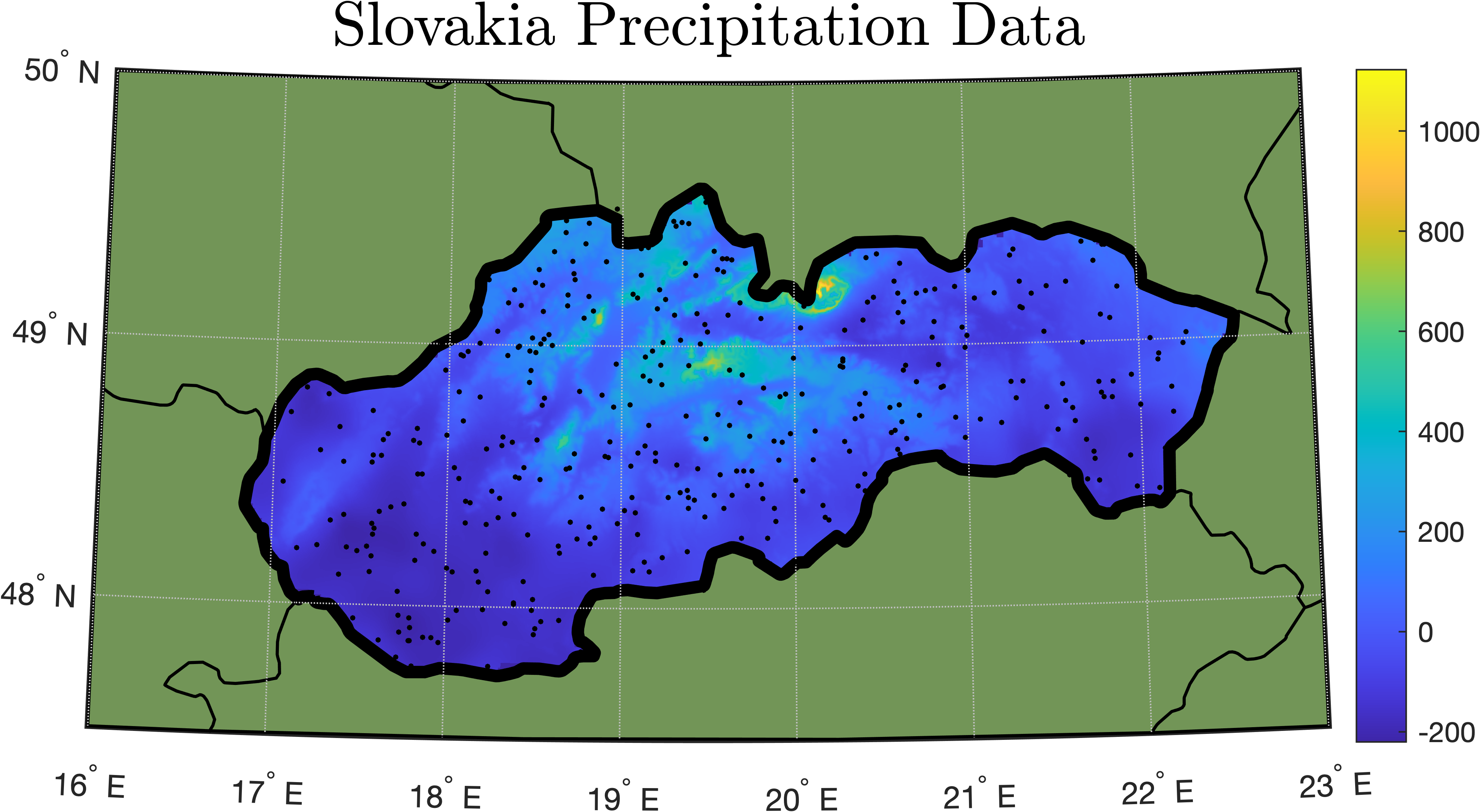
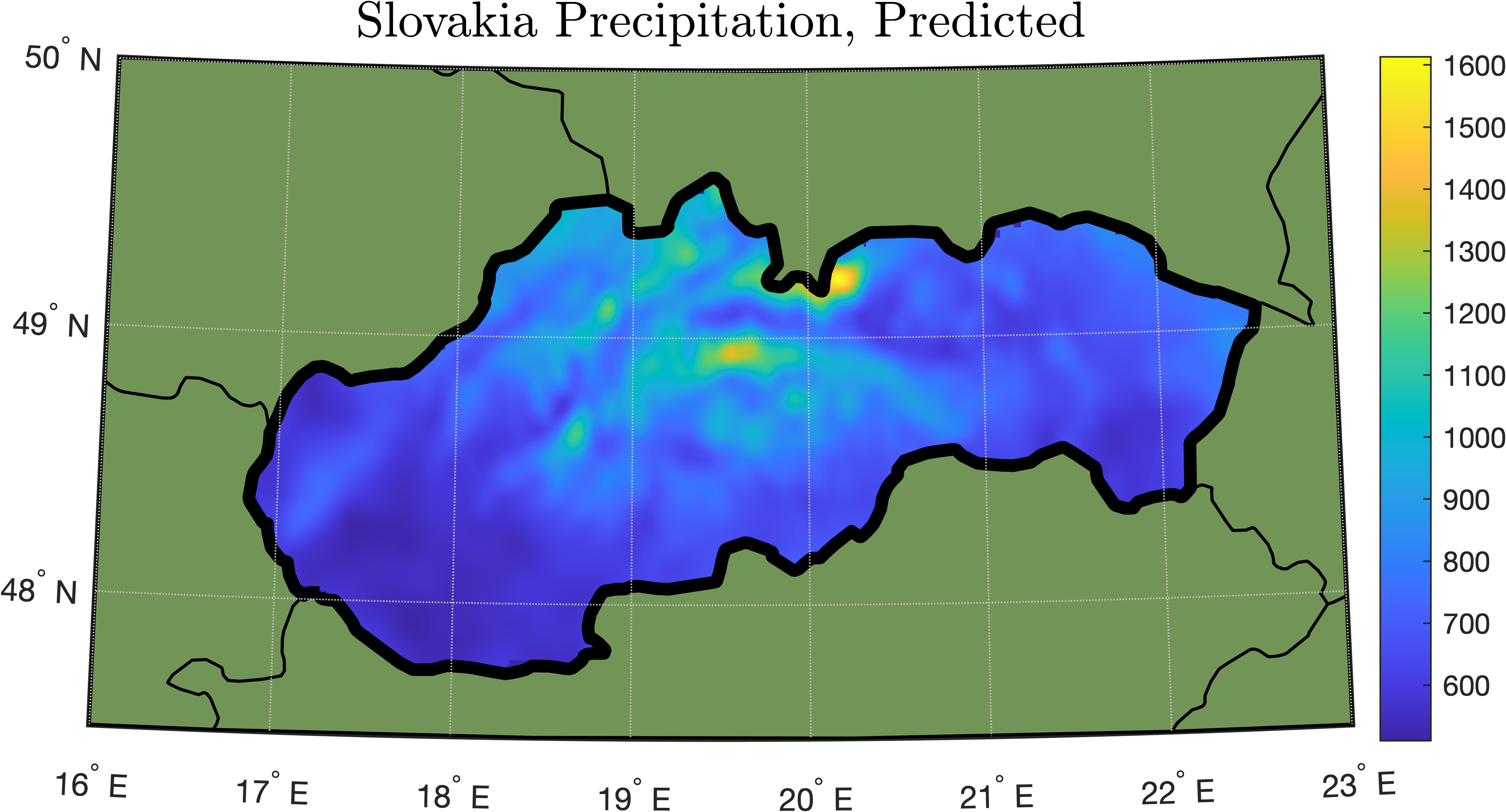
There are two ways to solve the problem faster using a kernel approximation: either $\tilde{\mathbf{K}}$ can be used in place of $\mathbf{K}$ when solving $(\mathbf{\tilde{K}}+\lambda\mathbf{I})^{-1}\mathbf{y}$ , or it can be used as a preconditioner to accelerate the iterative solution of $(\mathbf{K}+\lambda\mathbf{I})^{-1}\mathbf{y}$ . We explore the later approach because [AKM+17] already empirically shows the effectiveness of the former. While their modified RFF algorihm is different than ours in theory, we both make similar practical simplifications (see Section 5.1), which lead our empirically tested methods to be almost identical for the Gaussian kernel. Results on preconditioning are shown in Figure 4. Our modified RFF method leads to substantially faster convergence for a given number of random feature samples, which in turn leads to better downstream prediction error.

The superior performance of the modified RFF method can be explained theoretically: our method is designed to target the spectral approximation guarantee of Definition 1, which is guaranteed to ensure good preconditioning for $\mathbf{K}+\lambda\mathbf{I}$ [AKM+17]. On the other hand, the classical RFF method actually achieves better error than our method in other metrics like $\|\mathbf{K}-\tilde{\mathbf{K}}\|_{2}$ , both in theory [Tro15] and empirically (Figure 4). However, for preconditioning, such bounds will not necessarily ensure fast convergence. The key observation is that the spectral guarantee requires better approximation in the small eigenspaces of $\mathbf{K}$ . By more aggressively sampling higher frequencies that align with these directions (see Figure 2) the modified method obtains a better approximation.

5.1 Further details for experiments

We now describe some details of the modified random Fourier features sampling algorithm and preconditioning approach used in our empirical evaluation above.

Details of Sampling.

In our results, we employ simplified versions of the leverage score upper bounds from Theorems 1 and 2. In particular, in both of these theorems, the leverage score upper bound distributions are piecewise, following a different functions for frequencies above and below a certain cutoff $F$ . $F$ equals $6\sqrt{2}\sigma\cdot\sqrt{s}$ and $9\sqrt{2}\sigma\cdot{s}$ in Theorems 1 and 2, respectively. The bulk of each distribution is on values of $|\eta|\leq F$ , so we ignore the “tail” part of each distribution when sampling. This does not seem to significantly effect the experimental results. More over, using the empirical leverage score score distributions from Figure 1 as guidance, we used tighter values for $F$ than we were able to prove theoretically. For example, setting $F=4\sigma$ seems sufficient to capture the bulk of the Fourier sparse leverage score distribution for the Gaussian measure, so this is the value we used in our experiments. I.e. samples of $\eta$ were drawn uniformly from the ball $\{\eta:\|\eta\|_{2}<4\sigma\}$ .

When sampling we also use the same trick from [RR07] to achieve a real valued embedding, which makes it easier to work with the embedding downstream (e.g., when implementing the preconditioned solver). In particular, instead of including $C\cdot e^{-2\pi i\eta^{T}x}$ in the embedding, where $C$ is the appropriate constant as in Definition 3, we can include an entry equal of $C\cdot\cos(2\pi\eta^{T}x+\beta)$ where $\beta$ is a uniform random variable from $[0,2\pi]$ . It’s not hard to check that the corresponding real valued embedding will still satisfy $\mathbb{E}[\mathbf{G}^{*}\mathbf{G}]=\mathbf{K}$ , and experimentally, approximation quality does not appear to suffer.

Details of Preconditioning.

When solving $(\mathbf{K}+\lambda\mathbf{I})^{-1}\mathbf{z}$ with a preconditioner, each iteration of the preconditioned solver requires 1) computing $(\mathbf{\tilde{K}}+\lambda\mathbf{I})^{-1}\mathbf{z}$ for some vector $\mathbf{z}$ and 2) multiplying $\mathbf{K}+\lambda\mathbf{I}$ by a vector $\mathbf{w}$ . The first step can be done efficiently whenever $\mathbf{\tilde{K}}=\mathbf{G}^{*}\mathbf{G}$ where $\mathbf{G}\in\mathbb{C}^{n\times m}$ , which is the type of approximation we get from a random Fourier features method. In particular, let $\mathbf{G}=\mathbf{U}\boldsymbol{\Sigma}\mathbf{V}^{T}$ be $\mathbf{G}$ ’s singular value decomposition. Due to the simplification discussed above, $\mathbf{G}$ is always real-valued in our setting, and so is its SVD. We have $\mathbf{U}\in\mathbb{R}^{m\times m}$ , $\boldsymbol{\Sigma}\in\mathbb{R}^{m\times m}$ , and $\mathbf{V}\in\mathbb{R}^{n\times m}$ . The SVD can be computed in $O(m^{2}n)$ time and more importantly, this operation is very fast when $\mathbf{G}$ fits in memory, which is often possible even when $\mathbf{K}\in\mathbb{R}^{n\times n}$ does not. So, for both classical RFF preconditioning and modified RFF preconditioning, we choose values for $m$ that allow for fast computation of the SVD, and compute the decomposition as a preprocessing step.

Then, it is not hard to check that $(\mathbf{\tilde{K}}+\lambda\mathbf{I})^{-1}\mathbf{z}=\mathbf{V}\left(\boldsymbol{\Sigma}+\lambda\mathbf{I}_{m\times m}\right)^{-1}\mathbf{V}^{T}\mathbf{z}+\frac{1}{\lambda}(\mathbf{z}-\mathbf{V}^{T}\mathbf{z})$ , which can be computed in $O(mn)$ time. This is much faster than the cost of multiplying a vector by $\mathbf{K}+\lambda\mathbf{I}$ , so the cost of preconditioning ends up being a lower order term in the solver complexity: it increases the cost of each iteration by just a small factor.

6 Fourier Sparse Leverage Score Bounds – Proofs

We now prove our main Fourier sparse leverage score bounds under the Gaussian and Laplace densities (Theorems 1 and 2). When the minimum gap between frequencies in $f\in\mathcal{T}_{s}$ is bounded, we also give an improved bound based on Ingham’s inequality.

For notation in this section, we let $\|f\|_{2}^{2}=\int_{x\in\mathbb{R}}|f(x)|^{2}dx$ denote the $L_{2}$ norm of any complex valued function $f:\mathbb{R}\rightarrow\mathbb{C}$ . We denote the $L_{2}$ norm over an interval by $\|f\|_{[a,b]}^{2}=\int_{a}^{b}|f(x)|^{2}dx$ and the $L_{2}$ norm under any density $p$ over $\mathbb{R}$ as $\|f\|_{p}^{2}=\int_{x\in\mathbb{R}}|f(x)|^{2}\cdot p(x)\ dx$ .

6.1 Foundational bounds

We build on a number of existing bounds on the uniform density leverage scores and related concentration properties of an extended class of Fourier sparse functions with possibly complex frequencies. This class and its variants have been studied extensively, e.g., in [Tur84, Naz93, BE95, BE96, BE00, Kós08, Lub15, Erd17].

\displaystyle\mathcal{E}_{s}=\left\{f:f(x)=\sum_{j=1}^{s}a_{j}e^{\lambda_{j}x},a_{j}\in\mathbb{C},\lambda_{j}\in\mathbb{C}\right\}.

(11)

We also consider the subclasses where $\mathcal{E}_{s}^{+}$ and $\mathcal{E}_{s}^{-}$ , which are defined analogously to $\mathcal{E}_{s}$ but with frequencies $\lambda_{j}\in\mathbb{C}$ required to have non-negative (respectively, non-positive) real components. Note that our main class of interest $\mathcal{T}_{s}$ defined in (2) is contained in all three of these extended classes.

We first use a bound on the uniform density leverage score at any point $x$ on an interval, in terms of its distance from the edge of the interval.

Lemma 9.

For any $a,b\in\mathbb{R}$ with $a<b$ , $x\in(a,b)$ , and $f\in\mathcal{E}_{s}$ with $f\not\equiv 0$ :

\displaystyle\frac{|f(x)|^{2}}{\|f\|_{[a,b]}^{2}}\leq\frac{s}{\min(x-a,b-x)}.

Lemma 9 is stated, up to a constant factor $2$ in Theorem 7.1 [Erd17]. We prove it here for completeness and improve this constant.

Proof.

It is shown in equation (3) of [BE06] that for any $g\in\mathcal{E}_{s}$ with $g\not\equiv 0$ ,

\displaystyle\frac{|g(0)|^{2}}{\|g\|_{[-1,1]}^{2}}\leq s.

(12)

For $x\in(a,b)$ , let $\delta=\min(x-a,b-x)$ and $g(z)=f\left(x-\delta\cdot z\right)$ . Note that if $f\in\mathcal{E}_{s}$ and $f\not\equiv 0$ , we have $g\in\mathcal{E}_{s}$ and $g\not\equiv 0$ . Additionally, we have $g(0)=f(x)$ and $\|f\|_{[a,b]}^{2}\geq\|f\|_{[x-\delta,x+\delta]}^{2}=\delta\cdot\|g\|_{[-1,1]}^{2}$ . Applying (12) we then have:

\displaystyle\frac{|f(x)|^{2}}{\|f\|_{[a,b]}^{2}}\leq\frac{|g(0)|^{2}}{\delta\cdot\|g\|_{[-1,1]}^{2}}\leq\frac{s}{\delta},

which completes the proof. ∎

We note that Lemma 9 can be combined with Lemma 3.2 of [Den16], which tightens bounds proven in [Erd17] and [Kós08] to give the following bound for the uniform density leverage scores:

Corollary 10 (Uniform Density Leverage Score Bound).

Consider the uniform density $u(x)=\frac{1}{2\sigma}$ for $x\in[-\sigma,\sigma]$ , $u(x)=0$ otherwise, and let

\displaystyle\bar{\tau}_{s,z}(x)=\begin{cases}\frac{s}{\sigma-|x|}\text{ for }|x|\leq\sigma(1-\frac{4}{\pi s})\\ \frac{\pi}{4\sigma}s^{2}\text{ for }\sigma(1-\frac{4}{\pi s})<|x|\leq\sigma\\ 0\text{ for }|x|>\sigma\end{cases}

We have $\bar{\tau}_{s,u}(x)\geq\tau_{s,u}(x)$ for all $x\in\mathbb{R}$ and $\int_{-\infty}^{\infty}\bar{\tau}_{s,u}(x)\ dx=2s(1+\ln(\frac{\pi}{4}s))=O(s\ln s)$ .

Corollary 10 mirrors our Theorems 1 and 2, and as mentioned in Section 2, no upper bound can improve on the integral of $O(s\ln s)$ by more than a $\ln s$ factor. Understanding if this $\ln s$ can be eliminated or if it is necessary is an interesting open question.

We also employ a bound due to Turán [BE95], which plays a central role in his book [Tur84].

Lemma 11 (Turán’s lemma).

For any $g\in\mathcal{E}_{s}^{+}$ and $\alpha,\beta>0$ :

\displaystyle|g(0)|\leq\left(\frac{2e(\alpha+\beta)}{\beta}\right)^{s}\cdot\|g\|_{[\alpha,\alpha+\beta]}.

Turán’s lemma can be used to bound the growth of any function in $\mathcal{E}_{s}^{-}\supset\mathcal{T}_{s}$ outside of an interval in terms of its norm on that interval.

Lemma 12 (Lemma 12.2 [Erd17]).

For any $a\in\mathbb{R}$ , $d>0$ , $x\geq a+d$ , and $f\in\mathcal{E}_{s}^{-}$ :

\displaystyle|f(x)|\leq\left(\frac{2e(x-a)}{d}\right)^{s}\cdot\|f\|_{[a,a+d]}.

Proof.

Let $f\in{\mathcal{E}}_{s}^{-}$ . Let $g\in{\mathcal{E}}_{s}^{+}$ be defined by $g(t):=f(x-t)$ . We define $\alpha:=x-(a+d)$ and $\beta:=d$ . Applying Lemma 11 with $g\in{\mathcal{E}}_{s}^{+}$ we have

|f(x)|=|g(0)|\leq\left(\frac{2e(\alpha+\beta)}{\beta}\right)^{s}\|g\|_{[\alpha,\alpha+\beta]}=\left(\frac{2e(x-a)}{d}\right)^{s}\|f\|_{[a,a+d]}.

∎

Finally, our gap-based result apply to the following restricted class of $\mathcal{T}_{s}$ :

\displaystyle\mathcal{T}_{s,\gamma}=\left\{f:f(x)=\sum_{j=1}^{s}a_{j}e^{i\lambda_{j}x},a_{j}\in\mathbb{C},\lambda_{j}\in\mathbb{R}\text{ with }\min_{j,k}|\lambda_{k}-\lambda_{j}|\geq\gamma>0\right\}.

(13)

We denote the leverage score of this class with respect to a density $p$ by $\tau_{s,\gamma,p}(x)$ . In bounding these scores we use the following bound due to Ingham [Ing36]:

Lemma 13 (Ingram’s Inequality).

For any $\gamma>0$ , $f\in\mathcal{T}_{s,\gamma}$ with coefficients $a_{1},\ldots,a_{s}$ , and $T>\pi/\gamma,$

c_{1}(T,\gamma)\sum_{j=1}^{s}{|a_{j}|^{2}}\leq\|f\|_{[-T,T]}^{2}\leq c_{2}(T,\gamma)\sum_{j=1}^{s}{|a_{j}|^{2}}\,,

where

c_{1}(T,\gamma):=\frac{4T}{\pi}\left(1-\frac{\pi^{2}}{T^{2}\gamma^{2}}\right)\qquad\text{and}\qquad c_{2}(T,\gamma):=\frac{16T}{\pi}\left(1+\frac{\pi^{2}}{T^{2}\gamma^{2}}\right).

Setting $T=2\pi/\gamma$ in Ingram’s inequality gives:

Corollary 14.

For any $\gamma>0$ and $f\in\mathcal{T}_{s,\gamma}$ with coefficients $a_{1},\ldots,a_{s}$ , we have:

\displaystyle\frac{6}{\gamma}\sum_{j=1}^{s}{|a_{j}|^{2}}\leq\|f\|_{[-2\pi/\gamma,2\pi/\gamma]}^{2}\leq\frac{40}{\gamma}\sum_{j=1}^{s}{|a_{j}|^{2}}.

6.2 Bounds for the Gaussian density

Our leverage score bound for the Gaussian density (Theorem 1) is split into two components – a uniform bound on $\tau_{s,g}(x)$ for all $x\in\mathbb{R}$ (Claim 15) and a bound for $x$ restricted to have sufficiently large magnitude (Claim 16). Combining these two results gives the two part bound of Theorem 1. In this section we focus solely on the unit width Gaussian density: $g(x)=\frac{1}{\sqrt{\pi}}e^{-x^{2}}$ . Bounds under this density can immediately be translated into bounds for any width $\sigma>0$ via scaling. While they are not applicable to our algorithmic results, we give leverage score lower bounds as well, which help clarify the tightness of the bounds given.

Claim 15 (Gaussian Leverage Bound – Uniform Bound).

Letting $g(x)=\frac{1}{\sqrt{\pi}}e^{-x^{2}}$ , for all $x\in\mathbb{R}$ :

\displaystyle\frac{s}{3\pi}\leq\tau_{\mathcal{E}_{s},g}\leq e\cdot s.

As a consequence $\tau_{s,g}(x)\leq e\cdot s$ .

Proof.

For any $f\in\mathcal{E}_{s}$ and $a\in\mathbb{R}$ , define the shifted and weighted function $w_{a}(x)=f(x+a)\cdot e^{-(x+a)^{2}/2}.$ We can write:

	$\displaystyle w_{a}(x)$	$\displaystyle=\sum_{j=1}^{s}a_{j}e^{i\lambda_{j}(x+a)}e^{-x^{2}/2}e^{-a^{2}/2}e^{-xa}$
		$\displaystyle=e^{-x^{2}/2}\cdot\sum_{j=1}^{s}\left(a_{j}\cdot e^{i\lambda_{j}a}\cdot e^{-a^{2}/2}\right)\cdot e^{(i\lambda_{j}-a)x}.$

If we let $h_{a}(x)=\sum_{j=1}^{s}\left(a_{j}\cdot e^{i\lambda_{j}a}\cdot e^{-a^{2}/2}\right)\cdot e^{(i\lambda_{j}-a)x}$ we thus have $w_{a}(x)=e^{-x^{2}/2}\cdot h_{a}(x)$ and $h_{a}(x)\in\mathcal{E}_{s}$ . Applying Lemma 9 with $[a,b]=[-1,1]$ and $x=0$ gives:

\displaystyle\frac{|h_{a}(0)|^{2}}{\|h_{a}\|_{[-1,1]}^{2}}\leq s.

This gives

\displaystyle\frac{|w_{a}(0)|^{2}}{\|w_{a}\|_{2}^{2}}\leq\frac{|w_{a}(0)|^{2}}{\|w_{a}\|_{[-1,1]}^{2}}\leq s\cdot\frac{e^{0}}{e^{-1}}=e\cdot s.

Plugging in $a=x$ this gives:

\displaystyle\frac{|f(x)|^{2}\cdot\frac{1}{\sqrt{\pi}}e^{-x^{2}}}{\|f\|_{g}^{2}}=\frac{|w_{x}(0)|^{2}}{\|w_{x}\|_{2}^{2}}\leq e\cdot s.

where we use that $\|f\|_{g}^{2}=\frac{1}{\sqrt{\pi}}\|w_{a}\|_{2}^{2}$ for any $a$ due to the weighting $e^{-(x+a)^{2}/2}$ . Thus, we have $\tau_{\mathcal{E}_{s},g}(x)\leq e\cdot s$ , completing the upper bound.

For the lower bound, let $w_{t}\in{\mathcal{E}}_{s}$ be defined by

w_{t}(x):=f(x-t)e^{tx}\,,\qquad f(x):=\sum_{j=0}^{s-1}{e^{ijx}}\,.

We have

\displaystyle|w_{t}(t)|^{2}\cdot e^{-t^{2}}=s^{2}e^{2t^{2}}\cdot e^{-t^{2}}=s^{2}e^{t^{2}}.

(14)

Additionally,

	$\displaystyle\int_{{t\in\mathbb{R}}}{\|w_{t}(x)\|^{2}e^{-x^{2}}\,dx}$	$\displaystyle=\int_{{x\in\mathbb{R}}}{\|f(x-t)\|^{2}e^{2tx}e^{-x^{2}}\,dx}$
		$\displaystyle=e^{t^{2}}\int_{{x\in\mathbb{R}}}{\|f(x-t)\|^{2}e^{-(x-t)^{2}}\,dx}$
		$\displaystyle=e^{t^{2}}\int_{u\in\mathbb{R}}{\|f(u)\|^{2}e^{-u^{2}}\,du}.$

Since $f$ is a sum of complex exponentials with integer frequencies with period $2\pi$ , we can bound:

$\displaystyle\int_{{t\in\mathbb{R}}}{\|w_{t}(x)\|^{2}e^{-x^{2}}\,dx}$	$\displaystyle\leq e^{t^{2}}\int_{u\in\mathbb{R}}{\|f(u)\|^{2}e^{-u^{2}}\,du}$
	$\displaystyle\leq e^{t^{2}}\left(\int_{0}^{\pi}{\|f(u)\|^{2}e^{-u^{2}}\,du}\right)\cdot\left(2+2\sum_{k=1}^{\infty}{e^{-(k\pi)^{2}}}\right)$
	$\displaystyle\leq\,e^{t^{2}}\cdot 3\pi s,$	(15)

where the last bound follows from the fact that $\int_{0}^{\pi}{|f(x)|^{2}\,dx}=\pi s.$ Combining (14) and (6.2) we obtain the lower bound of the theorem.

∎

Claim 16 (Gaussian Leverage Bound – Large $x$ ).

Letting $g(x)=\frac{1}{\sqrt{\pi}}e^{-x^{2}}$ , when $|x|\geq 6\sqrt{s}$ ,

\displaystyle\tau_{s,g}(x)\leq e^{-x^{2}/2}.

Proof.

Applying Lemma 12 with $a=0$ and $d=x/2$ gives that for any $f\in\mathcal{T}_{s}$ :

\displaystyle\frac{|f(x)|^{2}}{\|f\|_{[0,x/2]}^{2}}\leq\left(4e\right)^{2s}.

This gives in turn that:

\displaystyle\tau_{s,g}(x)\leq\frac{e^{-x^{2}}\cdot(4e)^{2s}}{e^{-(x/2)^{2}}}\leq e^{-3/4\cdot x^{2}+6s}.

(16)

When $|x|\geq 6\sqrt{s}$ , $6s\leq\frac{x^{2}}{6}$ and so (17) gives $\tau_{s,g}(x)\leq e^{(-3/4+1/6)\cdot x^{2}}\leq e^{-x^{2}/2}$ , completing the claim. ∎

We can prove Theorem 1 directly from Claims 15 and 16.

Proof of Theorem 1.

For the Gaussian density $g(x)=\frac{1}{\sigma\sqrt{2\pi}}\cdot e^{-x^{2}/(2\sigma^{2})}$ :

\displaystyle\tau_{s,g}(x)=\sup_{f\in\mathcal{T}_{s}}\frac{|f(x)|^{2}\cdot e^{-x^{2}/(2\sigma^{2})}}{\int_{-\infty}^{\infty}|f(y)|^{2}e^{-y^{2}/(2\sigma^{2})}\ dy}

Let $\bar{g}(x)=\frac{1}{\sqrt{\pi}}e^{-x^{2}}$ be the Gaussian density with variance $1/2$ . For any $f\in\mathcal{T}_{s}$ , let $f_{\sigma}=f(\sqrt{2}\sigma\cdot x)$ . Note that $f_{\sigma}\in\mathcal{T}_{s}$ . We have:

\displaystyle\frac{|f(x)|^{2}\cdot e^{-x^{2}/(2\sigma^{2})}}{\int_{-\infty}^{\infty}|f(y)|^{2}e^{-y^{2}/(2\sigma^{2})}\ dy}=\frac{|f_{\sigma}(x/(\sqrt{2}\sigma))|^{2}\cdot e^{-x^{2}/(2\sigma^{2})}}{\int_{-\infty}^{\infty}|f_{\sigma}(y/(\sqrt{2}\sigma))|^{2}e^{-y^{2}/(2\sigma^{2})}\ dy}=\frac{|f_{\sigma}(x/(\sqrt{2}\sigma)|^{2}\cdot\bar{g}(x/(\sqrt{2}\sigma))}{\sqrt{2}\sigma\cdot\int_{-\infty}^{\infty}|f_{\sigma}(y)|^{2}\cdot\bar{g}(y)\ dy}.

Thus, $\tau_{s,g}(x)=\frac{1}{\sqrt{2}\sigma}\cdot\tau_{s,\bar{g}}(x/(\sqrt{2}\sigma))$ . By Claims 15 and 16, if we define:

\displaystyle\bar{\tau}_{s,g}(x)=\begin{cases}\frac{1}{\sqrt{2}\sigma}\cdot e^{-x^{2}/(4\sigma^{2})}\text{ for }|x|\geq 6\sqrt{2}\sigma\cdot\sqrt{s}\\ \frac{1}{\sqrt{2}\sigma}\cdot e\cdot s\text{ for }|x|\leq 6\sqrt{2}\sigma\cdot\sqrt{s}\end{cases}

we have

\displaystyle\tau_{s,g}(x)=\frac{1}{\sqrt{2}\sigma}\cdot\tau_{s,\bar{g}}(x/(\sqrt{2}\sigma))\leq\bar{\tau}_{s,g}(x).

Further,

\displaystyle\int_{\infty}^{\infty}\bar{\tau}_{s,g}(x)\ dx=\int_{-6\sqrt{2}\sigma\cdot\sqrt{s}}^{6\sqrt{2}\sigma\cdot\sqrt{s}}\frac{es}{\sqrt{2}\sigma}\ dx+\frac{2}{\sigma}\int_{6\sqrt{2}\sigma\cdot\sqrt{s}}^{\infty}e^{-x^{2}/(4\sigma^{2})}\ dx\leq 12es^{3/2}+1,

which completes the theorem. ∎

6.3 Bounds for the Laplace density

We now give bounds for the Laplace density, again focusing on the unit width case and then proving Theorem 2 via a simple scaling argument. Again, our bound is split into two components: a uniform bound for all $x$ and an improved bound for $x$ with large enough magnitude.

Claim 17 (Laplace Leverage Bound – Universal).

Letting $z(x)=\frac{1}{2}e^{-|x|}$ , for all $x\in\mathbb{R}$

\displaystyle\tau_{\mathcal{E}_{s},z}(x)\leq\frac{e^{2}\cdot s}{1+|x|}.

As a consequence, $\tau_{s,g}(x)\leq\frac{e^{2}\cdot s}{1+|x|}$ .

Proof.

Assume that $x$ is nonnegative. The same bound holds for negative $x$ , since for any $f\in\mathcal{E}_{s}$ , letting $f^{\prime}(x)=f(-x)$ , $f^{\prime}\in\mathcal{E}_{s}$ as well. For any $f\in\mathcal{T}_{s}$ define the weighted function $w(x)=f(x)\cdot\frac{1}{\sqrt{2}}e^{-x/2}$ . We can see that $w(x)\in\mathcal{E}_{s}$ as defined in (11) by writing:

\displaystyle w(x)

\displaystyle=\frac{1}{\sqrt{2}}\sum_{j=1}^{s}a_{j}e^{i\lambda_{j}x}e^{-x/2}=\frac{1}{\sqrt{2}}\sum_{j=1}^{s}a_{j}e^{(i\lambda_{j}-1/2)x}.

We define the ‘correctly’ weighted function $h(x)=f(x)\cdot\frac{1}{\sqrt{2}}e^{-|x|/2}$ . Note that for any $y\in[-1,0]$ , we have $h(y)\geq e^{-1}\cdot w(y)$ . Thus, we have:

\displaystyle\frac{|f(x)|^{2}\cdot\frac{1}{2}e^{-|x|}}{\|f\|_{z}^{2}}=\frac{|h(x)|^{2}}{\|h\|_{2}^{2}}\leq\frac{|h(x)|^{2}}{\|h\|_{[-1,2x+1]}^{2}}\leq e^{2}\cdot\frac{|w(x)|^{2}}{\|w\|_{[-1,2x+1]}^{2}}.

Applying Lemma 9 with $[a,b]=[1,2x+1]$ then gives:

\displaystyle\frac{|f(x)|^{2}\cdot\frac{1}{2}e^{-|x|}}{\|f\|_{z}^{2}}\leq e^{2}\cdot\frac{|w(x)|^{2}}{\|w\|_{[-1,2x+1]}^{2}}\leq\frac{e^{2}\cdot s}{1+x},

completing the claim. ∎

Claim 18 (Laplace Leverage Bound – Large $x$ ).

Letting $z(x)=\frac{1}{2}e^{-|x|}$ , when $|x|>18s$ ,

\displaystyle\tau_{s,z}(x)\leq e^{-|x|/6}.

Proof.

The proof is close to that of Claim 16 for the Gaussian density. As in Claim 17, assume without loss of generality that $x$ is nonnegative, so $x>12s$ .Applying Lemma 12 with $a=0$ and $d=x/2$ gives that for any $f\in\mathcal{T}_{s}$ :

\displaystyle\frac{|f(x)|^{2}}{\|f\|_{[0,x/2]}^{2}}\leq\left(4e\right)^{2s}.

This gives:

\displaystyle\tau_{s,z}(x)\leq\frac{e^{-x}\cdot(4e)^{2s}}{e^{-x/2}}\leq e^{-x/2+6s}.

(17)

When $x\geq 18s$ , $6s\leq\frac{x}{3}$ and so (17) gives $\tau_{s,g}(x)\leq e^{(-1/2+1/3)\cdot x^{2}}\leq e^{-x/6}$ , completing the claim. ∎

We can prove Theorem 2 directly from Claims 18 and 17.

Proof of Theorem 2.

As in the proof of Theorem 2, we can observe that for the Laplace density $z(x)=\frac{1}{\sqrt{2}\sigma}\cdot e^{-|x|\sqrt{2}/\sigma}$ , if we let $\bar{z}(x)=\frac{1}{2}e^{-|x|}$ be the density with variance $2$ , we have: $\tau_{s,z}(x)=\frac{\sqrt{2}}{\sigma}\cdot\tau_{s,\bar{z}}(x\sqrt{2}/\sigma)$ . By Claims 17 and 18, if we define:

\displaystyle\bar{\tau}_{s,z}(x)=\begin{cases}\frac{\sqrt{2}}{\sigma}\cdot e^{-|x|\sqrt{2}/(6\sigma)}\text{ for }|x|\geq 9\sqrt{2}\sigma\cdot{s}\\ \frac{\sqrt{2}}{\sigma}\cdot\frac{e^{2}\cdot s}{1+|x|\sqrt{2}/\sigma}\text{ for }|x|\leq 9\sqrt{2}\sigma\cdot{s}\end{cases}

we have

\displaystyle\tau_{s,z}(x)=\frac{1}{\sqrt{2}\sigma}\cdot\tau_{s,\bar{z}}(x\sqrt{2}/\sigma)\leq\bar{\tau}_{s,z}(x).

Further,

	$\displaystyle\int_{\infty}^{\infty}\bar{\tau}_{s,z}(x)\ dx$	$\displaystyle=\frac{2\sqrt{2}e^{2}}{\sigma}\cdot\int_{0}^{9\sqrt{2}\sigma{s}}\frac{s}{1+\|x\|\sqrt{2}/\sigma}\ dx+\frac{2\sqrt{2}}{\sigma}\int_{9\sqrt{2}\sigma\cdot{s}}^{\infty}e^{-x\sqrt{2}/(6\sigma)}\ dx$
		$\displaystyle=2e^{2}s\cdot\int_{0}^{18{s}}\frac{1}{1+x}\ dx+2\int_{18{s}}^{\infty}e^{-x/6}\ dx$
		$\displaystyle\leq 2e^{2}s\cdot\ln(18s+1)+1,$

which completes the theorem. ∎

6.4 Gap-based bounds

Finally, we show how to obtain tighter bounds for the Gaussian density when considering functions in $\mathcal{T}_{s,\gamma}$ , whose frequencies have minimum gap $\gamma>0$ (see (13)). We show:

Claim 19.

Letting $g(x)=\frac{1}{\sqrt{\pi}}e^{-x^{2}}$ , for all $x\in\mathbb{R}$ :

\displaystyle\tau_{s,\gamma,g}(x)\leq\left(\frac{\gamma}{6}\,e^{4\pi^{2}/\gamma^{2}}\right)\cdot se^{-x^{2}}.

The above leverage score upper bound is just a scaling of the data density $e^{-x^{2}}$ . For $\gamma=\Omega(1)$ , it integrates to $O(s)$ , within a constant factor of the lower bound $\int_{x\in\mathbb{R}}\tau_{s,\gamma,g}(x)\,dx\geq s$ given by restricting $\mathcal{T}_{s,\gamma}$ to just just a single fixed set of frequencies.

Claim 19 can be turned into a leverage score bound for the Gaussian density of any width, using the simple scaling argument of Theorem 1 giving:

Theorem 20 (Gaussian Leverage Bound – Gap Condition).

Consider the Gaussian density with variance $\sigma^{2}>0$ , $g(x)=\frac{1}{\sigma\sqrt{2\pi}}e^{-x^{2}/(2\sigma^{2})}$ , and let:

\displaystyle\bar{\tau}_{s,\gamma,g}(x)\leq\left(\frac{\gamma}{6}\,e^{4\pi^{2}/\gamma^{2}}\cdot s\right)\cdot\left(\frac{1}{\sqrt{2}\sigma}\cdot e^{-x^{2}/(2\sigma^{2})}\right).

We have $\tau_{s,\gamma,g}(x)\leq\bar{\tau}_{s,\gamma,g}(x)$ for all $x\in\mathbb{R}$ and $\int_{-\infty}^{\infty}\bar{\tau}_{s,\gamma,g}(x)dx=\frac{\gamma}{6}\,e^{4\pi^{2}/\gamma^{2}}\cdot\sqrt{\pi}s$ .

Proof of Claim 19.

Consider $f\in\mathcal{T}_{s,\gamma}$ with $f(x):=\sum_{j=1}^{s}{a_{j}e^{i\lambda_{j}x}},$ and $\min_{j,k}|\lambda_{k}-\lambda_{j}|\geq\gamma>0$ . Combining the Cauchy-Schwarz inequality with Ingham’s inequality (Lemma 13), we obtain

	$\displaystyle\|f(x)\|^{2}=\left\|\sum_{j=1}^{s}{a_{j}e^{i\lambda_{j}x}}\right\|^{2}$	$\displaystyle\leq\left(\sum_{j=1}^{s}{\left\|e^{i\lambda_{j}t}\right\|^{2}}\right)\left(\sum_{j=1}^{s}{\|a_{j}\|^{2}}\right)$
		$\displaystyle\leq\frac{\gamma s}{6}\int_{-2\pi/\gamma}^{2\pi/\gamma}{\left\|\sum_{j=1}^{s}{a_{j}e^{i\lambda_{j}x}}\right\|^{2}\,dx}$
		$\displaystyle\leq\left(\frac{\gamma}{6}\,e^{4\pi^{2}/\gamma^{2}}\right)s\int_{\mathbb{R}}{\|f(x)\|^{2}e^{-x^{2}}\,dx}.$

Hence

g(x)\cdot|f(x)|^{2}\leq\left(\frac{\gamma}{6}\,e^{4\pi^{2}/\gamma^{2}}\right)se^{-x^{2}}\cdot\|f\|_{g}^{2},

completing the claim. ∎

References

[AC20] Ben Adcock and Juan M. Cardenas. Near-optimal sampling strategies for multivariate function approximation on general domains. SIAM Journal on Mathematics of Data Science, 2020.
[AKK⁺20a] Naman Agarwal, Sham Kakade, Rahul Kidambi, Yin-Tat Lee, Praneeth Netrapalli, and Aaron Sidford. Leverage score sampling for faster accelerated regression and ERM. In Proceedings of the 31st International Conference on Algorithmic Learning Theory, volume 117, pages 22–47, 2020.
[AKK⁺20b] Thomas D. Ahle, Michael Kapralov, Jakob B. T. Knudsen, Rasmus Pagh, Ameya Velingker, David P. Woodruff, and Amir Zandieh. Oblivious sketching of high-degree polynomial kernels. In Proceedings of the 31st Annual ACM-SIAM Symposium on Discrete Algorithms (SODA), pages 141–160, 2020.
[AKM⁺17] Haim Avron, Michael Kapralov, Cameron Musco, Christopher Musco, Ameya Velingker, and Amir Zandieh. Random Fourier features for kernel ridge regression: approximation bounds and statistical guarantees. In Proceedings of the 34th International Conference on Machine Learning (ICML), pages 253–262, 2017.
[AKM⁺19] Haim Avron, Michael Kapralov, Cameron Musco, Christopher Musco, Ameya Velingker, and Amir Zandieh. A universal sampling method for reconstructing signals with simple Fourier transforms. In Proceedings of the 51st Annual ACM Symposium on Theory of Computing (STOC), 2019.
[AM15] Ahmed Alaoui and Michael W. Mahoney. Fast randomized kernel ridge regression with statistical guarantees. In Advances in Neural Information Processing Systems 28 (NeurIPS), pages 775–783, 2015.
[ANW14] Haim Avron, Huy Nguyen, and David Woodruff. Subspace embeddings for the polynomial kernel. In Advances in Neural Information Processing Systems 27 (NeurIPS), pages 2258–2266, 2014.
[Bac17] Francis Bach. On the equivalence between kernel quadrature rules and random feature expansions. Journal of Machine Learning Research, 18(21):1–38, 2017.
[BDMI14] Christos Boutsidis, Petros Drineas, and Malik Magdon-Ismail. Near-optimal column-based matrix reconstruction. SIAM Journal on Computing, 43(2):687–717, 2014.
[BE95] Peter Borwein and Tamás Erdélyi. Polynomials and polynomial inequalities, volume 161 of Graduate Texts in Mathematics. Springer-Verlag, New York, 1995.
[BE96] Peter Borwein and Tamás Erdélyi. A sharp Bernstein-type inequality for exponential sums. Journal für die reine und angewandte Mathematik, pages 127–141, 1996.
[BE00] Peter Borwein and Tamás Erdélyi. Pointwise Remez-and Nikolskii-type inequalities for exponential sums. Mathematische Annalen, 316(1):39–60, 2000.
[BE06] Peter Borwein and Tamás Erdélyi. Nikolskii-type inequalities for shift invariant function spaces. Proceedings of the American Mathematical Society, 134(11):3243–3246, 2006.
[CCM⁺15] Abdellah Chkifa, Albert Cohen, Giovanni Migliorati, Fabio Nobile, and Raul Tempone. Discrete least squares polynomial approximation with random evaluations - application to parametric and stochastic elliptic PDEs. ESAIM: M2AN, 49(3):815–837, 2015.
[CKPS16] Xue Chen, Daniel M. Kane, Eric Price, and Zhao Song. Fourier-sparse interpolation without a frequency gap. In Proceedings of the 57th Annual IEEE Symposium on Foundations of Computer Science (FOCS), pages 741–750, 2016. Full version at arXiv:1609.01361.
[CLM⁺15] Michael B. Cohen, Yin Tat Lee, Cameron Musco, Christopher Musco, Richard Peng, and Aaron Sidford. Uniform sampling for matrix approximation. In Proceedings of the 6th Conference on Innovations in Theoretical Computer Science (ITCS), pages 181–190, 2015.
[CM17] Albert Cohen and Giovanni Migliorati. Optimal weighted least-squares methods. SMIA Journal of Computational Mathematics, 3:181–203, 2017.
[CMM17] Michael B. Cohen, Cameron Musco, and Christopher Musco. Input sparsity time low-rank approximation via ridge leverage score sampling. In Proceedings of the 28th Annual ACM-SIAM Symposium on Discrete Algorithms (SODA), pages 1758–1777, 2017.
[CNW16] Michael B Cohen, Jelani Nelson, and David P Woodruff. Optimal approximate matrix product in terms of stable rank. In Proceedings of the 43rd International Colloquium on Automata, Languages and Programming (ICALP), 2016.
[CP17] Di Chen and Jeff M Phillips. Relative error embeddings of the Gaussian kernel distance. In International Conference on Algorithmic Learning Theory, pages 560–576, 2017.
[CP19a] Xue Chen and Eric Price. Active regression via linear-sample sparsification. Proceedings of the 32nd Annual Conference on Computational Learning Theory (COLT), 2019.
[CP19b] Xue Chen and Eric Price. Estimating the frequency of a clustered signal. In Proceedings of the 46th International Colloquium on Automata, Languages and Programming (ICALP), 2019.
[CVSK16] Sihen Chen, Rohan Varma, Aarti Singh, and Jelena Kovačcević. A statistical perspective of sampling scores for linear regression. In Proceedings of the 2016 IEEE International Symposium on Information Theory (ISIT), pages 1556–1560, 2016.
[Den16] S. Denisov. On the size of the polynomials orthonormal on the unit circle with respect to a measure which is a sum of the Lebesgue measure and $p$ point masses. Proceedings of the American Mathematical Society, 144:1029–1039, 2016.
[DM16] Petros Drineas and Michael W. Mahoney. RandNLA: Randomized numerical linear algebra. Communications of the ACM, 59(6), 2016.
[DMM06a] Petros Drineas, Michael W. Mahoney, and S. Muthukrishnan. Sampling algorithms for $\ell_{2}$ regression and applications. In Proceedings of the 17th Annual ACM-SIAM Symposium on Discrete Algorithms (SODA), pages 1127–1136, 2006.
[DMM06b] Petros Drineas, Michael W Mahoney, and Shanmugavelayutham Muthukrishnan. Subspace sampling and relative-error matrix approximation: Column-based methods. In Approximation, Randomization, and Combinatorial Optimization. Algorithms and Techniques, pages 316–326. Springer, 2006.
[DWH18] Michal Derezinski, Manfred K. K Warmuth, and Daniel J Hsu. Leveraged volume sampling for linear regression. In Advances in Neural Information Processing Systems 31 (NeurIPS). 2018.
[ELMM20] Yonina C. Eldar, Jerry Li, Cameron Musco, and Christopher Musco. Sample efficient toeplitz covariance estimation. Proceedings of the 31st Annual ACM-SIAM Symposium on Discrete Algorithms (SODA), 2020.
[Erd17] Tamás Erdélyi. Inequalities for exponential sums. Sbornik: Mathematics, 208(3):433–464, 2017.
[FB96] Ping Feng and Yoram Bresler. Spectrum-blind minimum-rate sampling and reconstruction of multiband signals. In Proceedings of the 1996 International Conference on Acoustics, Speech, and Signal Processing (ICASSP), pages 1688–1691, 1996.
[FSS19] Michaël Fanuel, Joachim Schreurs, and Johan AK Suykens. Nyström landmark sampling and regularized Christoffel functions. arXiv:1905.12346, 2019.
[GM13] Alex Gittens and Michael Mahoney. Revisiting the Nyström method for improved large-scale machine learning. In Proceedings of the 30th International Conference on Machine Learning (ICML), pages 567–575, 2013.
[GS12] Venkatesan Guruswami and Ali Kemal Sinop. Optimal column-based low-rank matrix reconstruction. In Proceedings of the 23rd Annual ACM-SIAM Symposium on Discrete Algorithms (SODA), pages 1207–1214. SIAM, 2012.
[HD15] Jerrad Hampton and Alireza Doostan. Coherence motivated sampling and convergence analysis of least squares polynomial chaos regression. Computer Methods in Applied Mechanics and Engineering, 290:73–97, 2015.
[HS93] Mark S. Handcock and Michael L. Stein. A Bayesian analysis of kriging. Technometrics, 35(4):403–410, 1993.
[Ing36] Albert Edward Ingham. Some trigonometrical inequalities with applications to the theory of series. Mathematische Zeitschrift, 41(1):367–379, 1936.
[KKP⁺20] Aku Kammonen, Jonas Kiessling, Petr Plecháč, Mattias Sandberg, and Anders Szepessy. Adaptive random Fourier features with Metropolis sampling. arXiv:2007.10683, 2020.
[Kós08] G. Kós. Two Turán type inequalities. Acta Mathematica Hungarica, 119(3):219–226, 2008.
[Kot33] Vladimir A. Kotelnikov. On the carrying capacity of the ether and wire in telecommunications. Material for the First All-Union Conference on Questions of Communication, Izd. Red. Upr. Svyazi RKKA, 1933.
[KS16] Rasmus Kyng and Sushant Sachdeva. Approximate Gaussian elimination for laplacians - fast, sparse, and simple. Proceedings of the 57th Annual IEEE Symposium on Foundations of Computer Science (FOCS), pages 573–582, 2016.
[Lan67] H. J. Landau. Sampling, data transmission, and the Nyquist rate. Proceedings of the IEEE, 55(10):1701–1706, 1967.
[LH12] Joseph D. Lakey and Jeffrey A. Hogan. On the numerical computation of certain eigenfunctions of time and multiband limiting. Numerical Functional Analysis and Optimization, 33(7-9):1095–1111, 2012.
[LHC⁺20] Fanghui Liu, Xiaolin Huang, Yudong Chen, Jie Yang, and Johan AK Suykens. Random Fourier features via fast surrogate leverage weighted sampling. In Proceedings of the $34^{th}$ AAAI Conference on Artificial Intelligence (AAAI), 2020.
[Lor83] Lee Lorch. Alternative proof of a sharpened form of Bernstein’s inequality for Legendre polynomials. Applicable Analysis, 14(3):237–240, 1983.
[LP61] Henry J. Landau and Henry O. Pollak. Prolate spheroidal wave functions, Fourier analysis and uncertainty – II. The Bell System Technical Journal, 40(1):65–84, 1961.
[LP62] Henry J. Landau and Henry O. Pollak. Prolate spheroidal wave functions, Fourier analysis and uncertainty – III: The dimension of the space of essentially time- and band-limited signals. The Bell System Technical Journal, 41(4):1295–1336, 1962.
[LP19] Jean B. Lasserre and Edouard Pauwels. The empirical Christoffel function with applications in data analysis. Advances in Computational Mathematics, 45(3):1439–1468, 2019.
[LS15] Yin Tat Lee and Aaron Sidford. Efficient inverse maintenance and faster algorithms for linear programming. In Proceedings of the 56th Annual IEEE Symposium on Foundations of Computer Science (FOCS), 2015.
[LTOS19] Zhu Li, Jean-Francois Ton, Dino Oglic, and Dino Sejdinovic. Towards a unified analysis of random Fourier features. Proceedings of the 36th International Conference on Machine Learning (ICML), 2019.
[Lub15] Doron S Lubinsky. Dirichlet orthogonal polynomials with laguerre weight. Journal of Approximation Theory, 194:146–156, 2015.
[LW80] Henry J. Landau and Harold Widom. Eigenvalue distribution of time and frequency limiting. Journal of Mathematical Analysis and Applications, 77(2):469–481, 1980.
[MDMW12] Michael W. Mahoney, Petros Drineas, Malik Magdon-Ismail, and David P. Woodruff. Fast approximation of matrix coherence and statistical leverage. Journal of Machine Learning Research, 13:3475–3506, 2012. Preliminary version in the 29th International Conference on Machine Learning (ICML).
[ME09] Moshe Mishali and Yonina C. Eldar. Blind multiband signal reconstruction: Compressed sensing for analog signals. IEEE Transactions on Signal Processing, 57(3):993–1009, 2009.
[Mig15] Giovanni Migliorati. Multivariate Markov-type and Nikolskii-type inequalities for polynomials associated with downward closed multi-index sets. Journal of Approximation Theory, 189:137 – 159, 2015.
[MM17] Cameron Musco and Christopher Musco. Recursive sampling for the Nyström method. In Advances in Neural Information Processing Systems 30 (NeurIPS), pages 3833–3845, 2017.
[MM20] Raphael A Meyer and Christopher Musco. The statistical cost of robust kernel hyperparameter tuning. In Advances in Neural Information Processing Systems 33 (NeurIPS), 2020.
[MMY15] Ping Ma, Michael W. Mahoney, and Bin Yu. A statistical perspective on algorithmic leveraging. Journal of Machine Learning Research, 16(1):861–911, 2015.
[MSW19] Michela Meister, Tamás Sarlós, and David Woodruff. Tight dimensionality reduction for sketching low degree polynomial kernels. In Advances in Neural Information Processing Systems 32 (NeurIPS), pages 9470–9481, 2019.
[Naz93] F. L. Nazarov. Local estimates for exponential polynomials and their applications to inequalities of the uncertainty principle type. (russian). Algebra i Analiz, 5(4):3–66, 1993. Translation in St. Petersburg Math. J. 5 (1994), no. 4, 663–717.
[Nev86] Paul Nevai. Géza Freud, orthogonal polynomials and Christoffel functions. a case study. Journal of Approximation Theory, 48(1):3 – 167, 1986.
[NM13] Markus Neteler and Helena Mitasova. Open source GIS: a GRASS GIS approach, volume 689. Springer Science & Business Media, 2013.
[Nyq28] Harry Nyquist. Certain topics in telegraph transmission theory. Transactions of the American Institute of Electrical Engineers, 47(2):617–644, 1928.
[OR14] Andrei Osipov and Vladimir Rokhlin. On the evaluation of prolate spheroidal wave functions and associated quadrature rules. Applied and Computational Harmonic Analysis, 36(1):108–142, 2014.
[PBV18] Edouard Pauwels, Francis Bach, and Jean-Philippe Vert. Relating leverage scores and density using regularized Christoffel functions. In Advances in Neural Information Processing Systems 31 (NeurIPS), pages 1670–1679, 2018.
[PP13] Ninh Pham and Rasmus Pagh. Fast and scalable polynomial kernels via explicit feature maps. In Proceedings of the 19th ACM SIGKDD International Conference on Knowledge Discovery and Data Mining (KDD), pages 239–247, 2013.
[PT20] Jeff M Phillips and Wai Ming Tai. The GaussianSketch for almost relative error kernel distance. In Proceedings of the 23rd International Workshop on Approximation Algorithms for Combinatorial Optimization Problems (APPROX), 2020.
[PVG⁺11] F. Pedregosa, G. Varoquaux, A. Gramfort, V. Michel, B. Thirion, O. Grisel, M. Blondel, P. Prettenhofer, R. Weiss, V. Dubourg, J. Vanderplas, A. Passos, D. Cournapeau, M. Brucher, M. Perrot, and E. Duchesnay. Scikit-learn: Machine learning in Python. Journal of Machine Learning Research, 12, 2011.
[RR07] Ali Rahimi and Benjamin Recht. Random features for large-scale kernel machines. In Advances in Neural Information Processing Systems 20 (NeurIPS), pages 1177–1184, 2007.
[RW06] Carl Edward Rasmussen and Christopher K. I. Williams. Gaussian Processes for Machine Learning. The MIT Press, 2006.
[RW12] Holger Rauhut and Rachel Ward. Sparse Legendre expansions via $\ell 1$ -minimization. Journal of Approximation Theory, 164(5):517 – 533, 2012.
[Sar06] Tamás Sarlós. Improved approximation algorithms for large matrices via random projections. In Proceedings of the 47th Annual IEEE Symposium on Foundations of Computer Science (FOCS), pages 143–152, 2006.
[Sha49] Claude E. Shannon. Communication in the presence of noise. Proceedings of the Institute of Radio Engineers, 37(1):10–21, 1949.
[SK19] Shahin Shahrampour and Soheil Kolouri. On sampling random features from empirical leverage scores: Implementation and theoretical guarantees. arXiv:1903.08329, 2019.
[SP61] David Slepian and Henry O. Pollak. Prolate spheroidal wave functions, Fourier analysis and uncertainty – I. The Bell System Technical Journal, 40(1):43–63, 1961.
[SS11] Daniel A. Spielman and Nikhil Srivastava. Graph sparsification by effective resistances. SIAM Journal on Computing, 40(6):1913–1926, 2011. Preliminary version in the 40th Annual ACM Symposium on Theory of Computing (STOC).
[Ste12] Michael L Stein. Interpolation of spatial data: some theory for kriging. Springer Science & Business Media, 2012.
[Tro15] Joel A. Tropp. An introduction to matrix concentration inequalities. Foundations and Trends in Machine Learning, 8(1-2):1–230, 2015.
[Tur84] Paul Turán. On a new method of analysis and its applications. John Wiley & Sons, 1984.
[WA13] Andrew Wilson and Ryan Adams. Gaussian process kernels for pattern discovery and extrapolation. In Proceedings of the 30th International Conference on Machine Learning (ICML), pages 1067–1075, 2013.
[Whi15] Edmund T. Whittaker. On the functions which are represented by the expansions of the interpolation theory. Proceedings of the Royal Society of Edinburgh, 35:181–194, 1915.
[Woo14] David P. Woodruff. Sketching as a tool for numerical linear algebra. Foundations and Trends in Theoretical Computer Science, 10(1–2):1–157, 2014.
[WS01] Christopher Williams and Matthias Seeger. Using the Nyström method to speed up kernel machines. In Advances in Neural Information Processing Systems 14 (NeurIPS), pages 682–688, 2001.
[XRY01] Hong Xiao, Vladimir Rokhlin, and Norman Yarvin. Prolate spheroidal wavefunctions, quadrature and interpolation. Inverse Problems, 17(4):805–838, 2001.

Appendix A Kernel Approximation – Omitted Proofs

As discussed in Section 3, our result on oblivious kernel embedding (Theorem 3) is based on a result from [AKM+17], which shows that strong kernel approximations can be obtained via random Fourier features methods which sample by the kernel ridge leverage scores of Definition 4:

Theorem 21 (Kernel Embedding via Leverage Score Sampling, [AKM+17]).

Let $s_{\lambda}$ denote the $\lambda$ -statistical dimension of $\mathbf{K}$ . Given a function $\bar{\tau}_{\lambda,\mathbf{K}}(\eta)$ with:

\bar{\tau}_{\lambda,\mathbf{K}}(\eta)\geq\tau_{\lambda,\mathbf{K}}(\eta)\text{ for all }\eta\in\mathbb{R}\text{ and }T\mathbin{\stackrel{{\scriptstyle\rm def}}{{=}}}\int_{\eta\in\mathbb{R}}\bar{\tau}_{\lambda,\mathbf{K}}(\eta)d\eta,

if we apply modified RFF sampling (Definition 3) with density $q(\eta)=\frac{\bar{\tau}_{\lambda,\mathbf{K}}(\eta)}{T}$ and sample size $m=\frac{3T\ln(16s_{\lambda}/\delta)}{\epsilon^{2}}$ , then with probability $\geq 1-\delta$ , $\mathbf{G}^{*}\mathbf{G}$ is an $(\epsilon,\lambda)$ -spectral approximation of $\mathbf{K}$ .

A.1 Kernel leverage score bounds via Fourier sparse approximation

To make use of Theorem 21, we need access to an upper bound $\bar{\tau}_{\lambda,\mathbf{K}}(\eta)$ on the kernel ridge leverage scores. We remark that $\int_{\eta\in\mathbb{R}}\tau_{\lambda,\mathbf{K}}(\eta)d\eta=\tr(\mathbf{K}+\lambda\mathbf{I})^{-1}\mathbf{K})=s_{\lambda}$ [AKM+17]. Thus, if $\bar{\tau}_{\lambda,\mathbf{K}}(\eta)$ is a tight bound, Theorem 21 yields an embedding dimension $m=\tilde{O}(s_{\lambda}/\epsilon^{2})$ . Our goal is to obtain a nearly tight bound by reducing the problem of bounding $\tau_{\lambda,\mathbf{K}}$ to that of bounding the Fourier sparse leverage score under the density $p_{k}$ given by the kernel Fourier transform. We prove:

Theorem 5.

\displaystyle\forall\eta\in\mathbb{R},\quad\tau_{\lambda,\mathbf{K}}(\eta)\leq(2+6s_{\lambda})\cdot\tau_{s,p_{k}}(\eta).

As discussed in Section 3, we prove Theorem 5 by first showing that any function $\mathbf{\Phi}\mathbf{w}$ in the span of our kernelized data points is well approximated by via an $O(s_{\lambda})$ sparse Fourier function. This Fourier sparse approximation result is based on the well-known fact that any matrix with bounded statistical dimension can be well approximated via projection onto a small subset of rows or columns [DMM06b, GS12, BDMI14]. In particular, we show via a simple reformulation of known results:

Theorem 22 (Row Subset Selection).

Consider the setting of Theorem 5. For $t=6\cdot\lceil s_{\lambda}\rceil$ , there exists a subset of $t$ indices ${i_{1}},\ldots,{i_{t}}\subseteq[n]$ and $\mathbf{Z}\in\mathbb{R}^{t\times n}$ such that, letting $\boldsymbol{\Phi}_{t}:\mathbb{C}^{t}\rightarrow L_{2}$ be the operator with $[\boldsymbol{\Phi}_{t}\mathbf{w}](\eta)=\sqrt{p_{k}(\eta)}\cdot\sum_{j=1}^{t}\mathbf{w}_{j}e^{-2\pi i\eta x_{i_{j}}}$ (i.e., the operator containing the $t$ columns of $\boldsymbol{\Phi}$ corresponding to the indices $i_{1},\ldots,i_{t}$ ):

\displaystyle\tr(\mathbf{K}-\mathbf{Z}^{T}\boldsymbol{\Phi}_{t}^{*}\boldsymbol{\Phi}_{t}\mathbf{Z})\leq 3\lambda s_{\lambda}\,\text{ and }\,\mathbf{Z}^{T}\boldsymbol{\Phi}_{t}^{*}\boldsymbol{\Phi}_{t}\mathbf{Z}\preceq\mathbf{K}.

Proof.

Let $\mathbf{B}\in\mathbb{R}^{n\times n}$ be any matrix squareroot of $\mathbf{K}$ with $\mathbf{B}^{T}\mathbf{B}=\mathbf{K}$ . Since $\mathbf{B}^{T}\mathbf{B}=\boldsymbol{\Phi}^{*}\boldsymbol{\Phi}$ it suffices to prove the existence of a subset of indices ${i_{1}},\ldots,{i_{t}}\subseteq[n]$ and a matrix $\mathbf{Z}\in\mathbb{R}^{t\times n}$ such that, letting $\mathbf{B}_{t}$ contain the columns of $\mathbf{B}$ corresponding to those indices:

\displaystyle\tr(\mathbf{K}-\mathbf{Z}^{T}\mathbf{B}_{t}^{T}\mathbf{B}_{t}\mathbf{Z})\leq 3\lambda s_{\lambda}\text{ and }\mathbf{Z}^{T}\mathbf{B}_{t}^{T}\mathbf{B}_{t}\mathbf{Z}\preceq\mathbf{K}.

(18)

Let $\mathbf{Z}=\mathbf{B}_{t}^{+}\mathbf{B}$ . Letting $\mathbf{P}_{t}=\mathbf{B}_{t}\mathbf{B}_{t}^{+}$ be the orthogonal projection matrix onto the columns of $\mathbf{B}_{t}$ , we can see that $\mathbf{Z}^{T}\mathbf{B}_{t}^{T}\mathbf{B}_{t}\mathbf{Z}=\mathbf{B}^{T}\mathbf{P}^{2}_{t}\mathbf{B}=\mathbf{B}^{T}\mathbf{P}_{t}\mathbf{B}$ . We first observe that for any $\mathbf{x}\in\mathbb{R}^{n}$ :

\displaystyle\mathbf{x}^{T}\mathbf{Z}^{T}\mathbf{B}_{t}^{T}\mathbf{B}_{t}\mathbf{Z}\mathbf{x}=\|\mathbf{P}_{t}\mathbf{B}\mathbf{x}\|_{2}^{2}\leq\|\mathbf{B}\mathbf{x}\|_{2}^{2}=\mathbf{x}^{T}\mathbf{K}\mathbf{x},

which proves that $\mathbf{Z}^{T}\mathbf{B}_{t}^{T}\mathbf{B}_{t}\mathbf{Z}\preceq\mathbf{K}$ , giving the second part of (18). To prove the first part of (18) we employ an optimal column-based matrix reconstruction result [GS12], Theorem 1.1, which shows that there exists a set of $s=6\cdot\lceil s_{\lambda}\rceil$ indices such that:

\displaystyle\|\mathbf{B}-\mathbf{B}_{t}\mathbf{Z}\|_{F}^{2}\leq 1.5\|\mathbf{B}-\mathbf{B}_{2\lceil s_{\lambda}\rceil}\|_{F}^{2},

(19)

where $\mathbf{B}_{2\lceil s_{\lambda}\rceil}$ is the best rank- $2\lceil s_{\lambda}\rceil$ approximation to $\mathbf{B}$ (given by projecting $\mathbf{B}$ onto its top $2\lceil s_{\lambda}\rceil$ singular vectors). Since $\mathbf{B}_{t}\mathbf{Z}$ is the projection of $\mathbf{B}$ onto the column space of $\mathbf{B}_{t}$ we can write via the Pythagorean theorem:

\displaystyle\|\mathbf{B}-\mathbf{B}_{t}\mathbf{Z}\|_{F}^{2}=\|\mathbf{B}\|_{F}^{2}-\|\mathbf{B}_{t}\mathbf{Z}\|_{F}^{2}=\tr(\mathbf{B}^{T}\mathbf{B})-\tr(\mathbf{Z}^{T}\mathbf{B}_{t}^{T}\mathbf{B}_{t}\mathbf{Z})=\tr(\mathbf{B}^{T}\mathbf{B}-\mathbf{Z}^{T}\mathbf{B}_{t}^{T}\mathbf{B}_{t}\mathbf{Z}).

Thus, in combination with (19), if we can show $\|\mathbf{B}-\mathbf{B}_{2\lceil s_{\lambda}\rceil}\|_{F}^{2}\leq 2\lambda s_{\lambda}$ , we will have

\displaystyle\tr(\mathbf{B}^{T}\mathbf{B}-\mathbf{Z}^{T}\mathbf{B}_{t}^{T}\mathbf{B}_{t}\mathbf{Z})\leq 3\lambda s_{\lambda},

yielding the first part of (18) and the theorem. This bound follows from the fact that $\|\mathbf{B}-\mathbf{B}_{\lceil 2s_{\lambda}\rceil}\|_{F}^{2}=\sum_{i=2\lceil s_{\lambda}\rceil+1}^{n}\lambda_{i}(\mathbf{K}).$ We can apply the following claim, which quantifies the eigenvalue decay of a matrix in terms of its statistical dimension:

Claim 23.

For any positive semidefinite $\mathbf{K}\in\mathbb{R}^{n\times n}$ with statistical dimension $s_{\lambda}$ :

\sum_{i=2\lceil s_{\lambda}\rceil+1}^{n}\lambda_{i}(\mathbf{K})\leq 2\lambda s_{\lambda}.

Proof.

Let $I_{\lambda}$ be the number of eigenvalues of $\mathbf{K}$ that are $\geq\lambda$ . We have:

	$\displaystyle s_{\lambda}=\sum_{i=1}^{n}\frac{\lambda_{i}(\mathbf{K})}{\lambda_{i}(\mathbf{K})+\lambda}$	$\displaystyle=\sum_{i=1}^{I_{\lambda}}\frac{\lambda_{i}(\mathbf{K})}{\lambda_{i}(\mathbf{K})+\lambda}+\sum_{i=I_{\lambda}+1}^{n}\frac{\lambda_{i}(\mathbf{K})}{\lambda_{i}(\mathbf{K})+\lambda}$
		$\displaystyle\geq\frac{1}{2}\cdot I_{\lambda}+\frac{1}{2\lambda}\sum_{i=I_{\lambda}+1}^{n}\lambda_{i}(\mathbf{K}),$

where the second line follows from that fact that $\lambda_{i}(\mathbf{K})\geq\lambda$ for $i\leq I_{\lambda}$ and $\lambda_{i}(\mathbf{K})<\lambda$ for $i>I_{\lambda}$ Rearranging we have $2\lceil s_{\lambda}\rceil\geq 2s_{\lambda}\geq I_{\lambda}$ and $2s_{\lambda}\geq\frac{1}{\lambda}\sum_{i=I_{\lambda}+1}^{n}\lambda_{i}(\mathbf{K})$ , and in turn:

\displaystyle 2s_{\lambda}\geq\frac{1}{\lambda}\sum_{i=2\lceil s_{\lambda}\rceil+1}^{n}\lambda_{i}(\mathbf{K})\implies 2\lambda s_{\lambda}\geq\sum_{i=2\lceil s_{\lambda}\rceil+1}^{n}\lambda_{i}(\mathbf{K}).

∎

Claim 23 directly gives that $\|\mathbf{B}-\mathbf{B}_{2\lceil s_{\lambda}\rceil}\|_{F}^{2}=\sum_{i=2\lceil s_{\lambda}\rceil+1}^{n}\lambda_{i}(\mathbf{K})\leq 2\lambda s_{\lambda}$ , completing the proof of Theorem 22. ∎

Proof of Theorem 5.

Applying Theorem 22 we can bound the kernel leverage score by breaking the function $\boldsymbol{\Phi}\mathbf{w}$ into its projection onto $\boldsymbol{\Phi}_{t}$ , which after a change of density is a $t=\lceil 6s_{\lambda}\rceil$ -sparse Fourier function in $\mathcal{T}_{t}$ , and the residual.

	$\displaystyle\tau_{\lambda,\mathbf{K}}(\eta)=\sup_{\mathbf{w}\in\mathbb{C}^{n},\mathbf{w}\neq 0}\frac{\|[\boldsymbol{\Phi}\mathbf{w}](\eta)\|^{2}}{\\|\boldsymbol{\Phi}\mathbf{w}\\|_{2}^{2}+\lambda\\|\mathbf{w}\\|_{2}^{2}}$	$\displaystyle\leq\frac{2\|[\boldsymbol{\Phi}_{t}\mathbf{Z}\mathbf{w}](\eta)\|^{2}}{\\|\boldsymbol{\Phi}\mathbf{w}\\|_{2}^{2}+\lambda\\|\mathbf{w}\\|_{2}^{2}}+\frac{2\|[\boldsymbol{\Phi}\mathbf{w}](\eta)-[\boldsymbol{\Phi}_{t}\mathbf{Z}\mathbf{w}](\eta)\|^{2}}{\\|\boldsymbol{\Phi}\mathbf{w}\\|_{2}^{2}+\lambda\\|\mathbf{w}\\|_{2}^{2}}$
		$\displaystyle\leq\frac{2\|[\boldsymbol{\Phi}_{t}\mathbf{Z}\mathbf{w}](\eta)\|^{2}}{\\|\boldsymbol{\Phi}\mathbf{w}\\|_{2}^{2}}+\frac{2\|[\boldsymbol{\Phi}\mathbf{w}](\eta)-[\boldsymbol{\Phi}_{t}\mathbf{Z}\mathbf{w}](\eta)\|^{2}}{\lambda\\|\mathbf{w}\\|_{2}^{2}}.$		(20)

Since by Theorem 22, $\mathbf{Z}^{T}\boldsymbol{\Phi}_{t}^{*}\boldsymbol{\Phi}_{t}\mathbf{Z}\preceq\mathbf{K}$ we have

\|\boldsymbol{\Phi}\mathbf{w}\|_{2}^{2}=\mathbf{w}^{T}\mathbf{K}\mathbf{w}\geq\mathbf{w}^{T}\mathbf{Z}^{T}\boldsymbol{\Phi}_{t}^{*}\boldsymbol{\Phi}_{t}\mathbf{Z}\mathbf{w}=\|\boldsymbol{\Phi}_{t}\mathbf{Z}\mathbf{w}\|_{2}^{2},

which combined with (A.1) gives:

	$\displaystyle\tau_{\lambda,\mathbf{K}}(\eta)$	$\displaystyle\leq\frac{2\|[\boldsymbol{\Phi}_{t}\mathbf{Z}\mathbf{w}](\eta)\|^{2}}{\\|\boldsymbol{\Phi}_{t}\mathbf{Z}\mathbf{w}\\|_{2}^{2}}+\frac{2\|[\boldsymbol{\Phi}\mathbf{w}](\eta)-[\boldsymbol{\Phi}_{t}\mathbf{Z}\mathbf{w}](\eta)\|^{2}}{\lambda\\|\mathbf{w}\\|_{2}^{2}}$
		$\displaystyle\leq 2\tau_{t,p_{k}}(\eta)+\frac{2\|[\boldsymbol{\Phi}\mathbf{w}](\eta)-[\boldsymbol{\Phi}_{t}\mathbf{Z}\mathbf{w}](\eta)\|^{2}}{\lambda\\|\mathbf{w}\\|_{2}^{2}}.$		(21)

The second bound follows from the fact that $\frac{[\boldsymbol{\Phi}_{t}\mathbf{Z}\mathbf{w}](\eta)}{\sqrt{p_{k}(\eta)}}\in\mathcal{T}_{t}$ . It remains to bound the second term of (A.1). Let $\mathbf{z}(\eta)\in\mathbb{C}^{n}$ be the vector with $\mathbf{z}(\eta)_{j}=\left[e^{-2\pi i\eta x_{j}}-\sum_{k=1}^{t}\mathbf{Z}_{k,j}\cdot e^{-2\pi i\eta x_{i_{k}}}\right]\cdot\sqrt{p_{k}(\eta)}$ . Then we can bound via Cauchy-Schwarz:

\displaystyle\frac{|[\boldsymbol{\Phi}\mathbf{w}](\eta)-[\boldsymbol{\Phi}_{s}\mathbf{Z}\mathbf{w}](\eta)|^{2}}{\lambda\|\mathbf{w}\|_{2}^{2}}=\frac{|\mathbf{z}(\eta)^{*}\mathbf{w}|^{2}}{\lambda\|\mathbf{w}\|_{2}^{2}}\leq\frac{\|\mathbf{z}(\eta)\|_{2}^{2}}{\lambda}.

(22)

We bound $\|\mathbf{z}(\eta)\|_{2}^{2}$ as:

Claim 24.

Let $\mathbf{z}(\eta)\in\mathbb{C}^{n}$ be as defined above. $\|\mathbf{z}(\eta)\|_{2}^{2}\leq\tau_{t+1,p_{k}}(\eta)\cdot 3\lambda s_{\lambda}$ .

Combining Claim 24 with (A.1) and (22) yields:

\displaystyle\tau_{\lambda,\mathbf{K}}(\eta)

\displaystyle\leq 2\tau_{t,p_{k}}(\eta)+6\tau_{t+1,p_{k}}(\eta)\cdot s_{\lambda}\leq(2+6s_{\lambda})\cdot\tau_{6t+1,p_{k}}(\eta),

which completes the theorem after recalling that we set $t=\lceil s_{\lambda}\rceil$ in Theorem 22. ∎

Proof of Claim 24.

Consider the function $g_{j}(\eta)=\mathbf{z}(\eta)_{j}$ and $g(\eta)=\sum_{j=1}^{n}|g_{j}(\eta)|^{2}=\|\mathbf{z}(\eta)\|_{2}^{2}$ .

\displaystyle g_{j}(\eta)=\left[e^{-2\pi i\eta x_{j}}-\sum_{k=1}^{s}\mathbf{Z}(k,j)\cdot e^{-2\pi i\eta x_{i_{k}}}\right]\cdot\sqrt{p_{k}(\eta)}

and thus, $h(\eta)\mathbin{\stackrel{{\scriptstyle\rm def}}{{=}}}\frac{g_{j}(\eta)}{\sqrt{p_{k}(\eta)}}\in\mathcal{T}_{t+1}$ and so:

\displaystyle\frac{|g_{j}(\eta)|^{2}}{\|g_{j}\|_{2}^{2}}=\frac{p_{k}(\eta)\cdot|h(\eta)|^{2}}{\|h\|_{p_{k}}^{2}}\leq\tau_{t+1,p_{k}}(\eta).

This gives:

	$\displaystyle\\|\mathbf{z}(\eta)\\|_{2}^{2}=\sum_{j=1}^{n}\|g_{j}(\eta)\|^{2}$	$\displaystyle\leq\tau_{t+1,p_{k}}(\eta)\cdot\sum_{j=1}^{n}\\|g_{j}\\|_{2}^{2}$
		$\displaystyle=\tau_{t+1,p_{k}}(\eta)\cdot\tr(\mathbf{K}-\mathbf{Z}^{T}\boldsymbol{\Phi}_{s}^{*}\boldsymbol{\Phi}_{s}\mathbf{Z})$
		$\displaystyle\leq\tau_{t+1,p_{k}}(\eta)\cdot 3s_{\lambda},$

where the last bound follows from Theorem 22. ∎

A.2 Oblivious kernel embedding via keverage score-based RFF

We finally combine our Fourier sparse leverage score bounds of Theorems 1 and 2 with the kernel ridge leverage score bound of Theorem 5 and the leverage score sampling result of Theorem 21 to give oblivious kernel embedding results for the kernels corresponding to the Fourier transforms of the Gaussian and Laplace densities – i.e., the Gaussian and Cauchy (rational quadratic) kernel.

Corollary 25 (Modified RFF Embedding – Gaussian Kernel).

Consider any set of points $x_{1},\ldots,x_{n}\in\mathbb{R}$ and the associated Gaussian kernel matrix $\mathbf{K}\in\mathbb{R}^{n\times n}$ with $\mathbf{K}_{i,j}=e^{-(x_{i}-x_{j})^{2}/(2\sigma^{2})}$ . Let $s_{\lambda}$ be the $\lambda$ -statistical dimension of $\mathbf{K}$ , $s=6\lceil s_{\lambda}\rceil+1$ , and $q(\eta)$ be the density proportional to:

\displaystyle q(\eta)\propto\begin{cases}e^{-\eta^{2}\cdot\pi^{2}\cdot\sigma^{2}}\text{ for }|\eta|\geq\frac{3\sqrt{2}}{\sigma\pi}\cdot\sqrt{s}\\ e\cdot s\text{ for }|\eta|\leq\frac{3\sqrt{2}}{\sigma\pi}\cdot\sqrt{s}.\end{cases}

The modified RFF embedding (Def. 3) with density $q(\eta)$ and sample size $m=O\left(\frac{s_{\lambda}^{5/2}\cdot\log(s_{\lambda}/\delta)}{\epsilon^{2}}\right)$ , satisfies $\mathbf{G}^{*}\mathbf{G}$ is an $(\epsilon,\lambda)$ -spectral approximation of $\mathbf{K}$ with probability $\geq 1-\delta$ . The embedding $\mathbf{g}(x_{i})\in\mathbb{C}^{m}$ , can be constructed obliviously in $O(m)$ time.

Proof.

For the Gaussian kernel with width $\sigma$ , the Fourier transform density is also Gaussian with variance $\frac{1}{4\pi^{2}\sigma^{2}}$ :

\displaystyle p_{k}(\eta)=\int_{t\in\mathbb{R}}e^{2\pi i\eta t}e^{-\frac{t^{2}}{2\sigma^{2}}}dt=\sigma\sqrt{2\pi}\cdot e^{-2\sigma^{2}\pi^{2}\eta^{2}}.

Applying Theorem 5 we have: $\tau_{\lambda,\mathbf{K}}(\eta)\leq(2+6s_{\lambda})\cdot\tau_{s,p_{k}}(\eta)$ for $s=6\lceil s_{\lambda}\rceil+1$ . In turn, applying Theorem 1 gives $\tau_{\lambda,\mathbf{K}}(\eta)\leq\bar{\tau}_{\lambda,\mathbf{K}}(\eta)$ where:

\displaystyle\bar{\tau}_{\lambda,\mathbf{K}}(\eta)=\begin{cases}(2+6s_{\lambda})\cdot\pi\sqrt{2}\cdot\sigma\cdot e^{-\eta^{2}\cdot\pi^{2}\cdot\sigma^{2}}\text{ for }|\eta|\geq\frac{3\sqrt{2}}{\sigma\pi}\cdot\sqrt{s}\\ (2+6s_{\lambda})\cdot\pi\sqrt{2}e\cdot\sigma\cdot s\text{ for }|\eta|\leq\frac{3\sqrt{2}}{\sigma\pi}\cdot\sqrt{s}.\end{cases}

Thus, by Theorem 21, if we let $q(\eta)$ be the density proportional to $\bar{\tau}_{\lambda,\mathbf{K}}(\eta)$ , a random Fourier features approximation satisfies the guarantee of the Theorem with sample size $m$ given by:

\displaystyle m=O\left(\frac{\int_{\eta\in\mathbb{R}}\bar{\tau}_{\lambda,\mathbf{K}}(\eta)d\eta\,\cdot\log(s_{\lambda}/\delta)}{\epsilon^{2}}\right)=O\left(\frac{s_{\lambda}^{5/2}\cdot\log(s_{\lambda}/\delta)}{\epsilon^{2}}\right),

since by Theorem 1, $\int_{\eta\in\mathbb{R}}\bar{\tau}_{\lambda,\mathbf{K}}(\eta)d\eta=(2+6s_{\lambda})\cdot O(s^{3/2})=O(s_{\lambda}^{5/2})$ .

Finally, we observe that $q(\eta)$ is just a mixture of a Gaussian density with a uniform density, and hence can be sampled from in $O(1)$ time. Thus each embedding $\mathbf{g}(x_{i})\in\mathbb{C}^{m}$ can be constructed obliviously in $O(m)$ time. ∎

We give a very similar result for the Cauchy (also known as rational quadratic) kernel using our Laplacian distribution leverage score bound of Theorem 2.

Corollary 26 (Modified RFF Embedding – Cauchy Kernel).

Consider any set of points $x_{1},\ldots,x_{n}\in\mathbb{R}$ and the associated Cauchy kernel matrix $\mathbf{K}\in\mathbb{R}^{n\times n}$ with $\mathbf{K}_{i,j}=\frac{1}{1+(x_{i}-x_{j})^{2}/\sigma^{2}}$ . Let $s_{\lambda}$ be the $\lambda$ -statistical dimension of $\mathbf{K}$ , $s=6\lceil s_{\lambda}\rceil+1$ , and $q(\eta)$ be the density proportional to:

\displaystyle q(\eta)\propto\begin{cases}e^{-|\eta|\cdot\sigma\pi/3}\text{ for }|\eta|\geq\frac{9s}{\sigma\pi}\\ \frac{e^{2}s}{1+|\eta|\cdot 2\sigma\pi}\text{ for }|\eta|\leq\frac{9s}{\sigma\pi}.\end{cases}

The modified RFF embedding (Def. 3) with density $q(\eta)$ and sample size $m=O\left(\frac{s_{\lambda}^{2}\log(s_{\lambda})\cdot\log(s_{\lambda}/\delta)}{\epsilon^{2}}\right)$ satisfies $\mathbf{G}^{*}\mathbf{G}$ is an $(\epsilon,\lambda)$ -spectral approximation of $\mathbf{K}$ with probability $\geq 1-\delta$ . The embedding $\mathbf{g}(x_{i})\in\mathbb{C}^{m}$ , can be constructed obliviously in $O(m)$ time.

Proof.

For the Cauchy kernel with width $\sigma$ , the Fourier transform density is a Laplace density:

\displaystyle p_{k}(\eta)=\int_{t\in\mathbb{R}}e^{2\pi i\eta t}\frac{1}{1+(t/\sigma)^{2}}dt=\sigma\pi\cdot e^{-|\eta|\cdot 2\sigma\pi}.

Applying Theorem 5 we have: $\tau_{\lambda,\mathbf{K}}(\eta)\leq(2+6s_{\lambda})\cdot\tau_{s,p_{k}}(\eta)$ for $s=6\lceil s_{\lambda}\rceil+1$ . In turn, applying Theorem 2 gives $\tau_{\lambda,\mathbf{K}}(\eta)\leq\bar{\tau}_{\lambda,\mathbf{K}}(\eta)$ where:

\displaystyle\bar{\tau}_{\lambda,\mathbf{K}}(\eta)=\begin{cases}(2+6s_{\lambda})\cdot 2\sigma\pi\cdot e^{-|\eta|\cdot\sigma\pi/3}\text{ for }|\eta|\geq\frac{9s}{\sigma\pi}\\ (2+6s_{\lambda})\cdot 2\sigma\pi\cdot\frac{e^{2}s}{1+|\eta|\cdot 2\sigma\pi}\text{ for }|\eta|\leq\frac{9s}{\sigma\pi}.\end{cases}

\displaystyle m=O\left(\frac{\int_{\eta\in\mathbb{R}}\bar{\tau}_{\lambda,\mathbf{K}}(\eta)d\eta\,\cdot\log(s_{\lambda}/\delta)}{\epsilon^{2}}\right)=O\left(\frac{s_{\lambda}^{2}\log(s_{\lambda})\cdot\log(s_{\lambda}/\delta)}{\epsilon^{2}}\right),

since by Theorem 2, $\int_{\eta\in\mathbb{R}}\bar{\tau}_{\lambda,\mathbf{K}}(\eta)d\eta=(2+6s_{\lambda})\cdot O(s\log s)=O(s_{\lambda}^{2}\log s_{\lambda})$ .

Finally, observe that $q(\eta)$ is just a mixture of a Laplacian density with a density of the form $\frac{1}{1+|\eta|\cdot 2\sigma\pi}$ . Both can be sampled from in $O(1)$ time using, e.g., inverse transform sampling. Thus each embedding $\mathbf{g}(x_{i})$ can be constructed obliviously in $O(m)$ time. ∎

A.3 Final embedding via random projection

Corollaries 25 and 26 give oblivious embeddings into $\poly(s_{\lambda})$ dimensions via leverage score-based RFF sampling. These oblivious embeddings can be further compressed via standard oblivious random projection time to give an oblivious embedding algorithm achieving the target dimension, linear in $s_{\lambda}$ . Specifically we apply a stable rank approximate matrix multiplication result from [CNW16]:

Theorem 27 (Random Projection Spectral Approximation).

For any $\mathbf{Z}\in\mathbb{R}^{n\times s}$ and $\mathbf{M}=\mathbf{ZZ}^{T}$ with $\lambda$ -statistical dimension $s_{\lambda}$ , if $\boldsymbol{\Pi}\in\mathbb{R}^{s\times m}$ has independent sub-Gaussian entries with variance $1/m$ for $m=O\left(\frac{s_{\lambda}+\log(1/\delta)}{\epsilon^{2}}\right)$ , then with probability $\geq 1-\delta$ , $\mathbf{Z}\boldsymbol{\Pi}\boldsymbol{\Pi}^{T}\mathbf{Z}^{T}$ is an $(\epsilon,\lambda)$ -spectral approximation of $\mathbf{M}$ .

A simple example of $\boldsymbol{\Pi}$ that satisfies the theorem is one with independent $\pm 1/\sqrt{m}$ entries. See [CNW16] for more details on sketching matrices that may be used, including sparse ones.

Proof.

Let $\mathbf{B}=(\mathbf{M}+\lambda\mathbf{I})^{-1/2}\mathbf{Z}$ . To prove the theorem it suffices to show that with probability $\geq 1-\delta$ , $\|\mathbf{B}\boldsymbol{\Pi}\boldsymbol{\Pi}^{T}\mathbf{B}^{T}-\mathbf{BB}^{T}\|_{2}\leq\epsilon$ as this gives:

	$\displaystyle-\epsilon\mathbf{I}$	$\displaystyle\preceq\mathbf{B}\boldsymbol{\Pi}\boldsymbol{\Pi}^{T}\mathbf{B}^{T}-\mathbf{BB}^{T}\preceq\epsilon\mathbf{I}$
	$\displaystyle-\epsilon(\mathbf{M}+\lambda\mathbf{I})$	$\displaystyle\preceq\mathbf{Z}\boldsymbol{\Pi}\boldsymbol{\Pi}^{T}\mathbf{Z}^{T}-\mathbf{ZZ}^{T}\preceq\epsilon(\mathbf{M}+\lambda\mathbf{I})$
	$\displaystyle\mathbf{M}-\epsilon(\mathbf{M}+\lambda\mathbf{I})$	$\displaystyle\preceq\mathbf{Z}\boldsymbol{\Pi}\boldsymbol{\Pi}^{T}\mathbf{Z}^{T}\preceq\mathbf{M}+\epsilon(\mathbf{M}+\lambda\mathbf{I})$
	$\displaystyle(1-\epsilon)(\mathbf{M}+\lambda\mathbf{I})$	$\displaystyle\preceq\mathbf{Z}\boldsymbol{\Pi}\boldsymbol{\Pi}^{T}\mathbf{Z}^{T}+\lambda\mathbf{I}\preceq(1+\epsilon)(\mathbf{M}+\lambda\mathbf{I}),$

which gives the theorem.

To prove that $\|\mathbf{B}\boldsymbol{\Pi}\boldsymbol{\Pi}^{T}\mathbf{B}^{T}-\mathbf{BB}^{T}\|_{2}\leq\epsilon$ with probability $\geq 1-\delta$ we invoke Theorem 1 of [CNW16], which gives that for our setting of $m$ , with probability $\geq 1-\delta$ :

\displaystyle\|\mathbf{B}\boldsymbol{\Pi}\boldsymbol{\Pi}^{T}\mathbf{B}^{T}-\mathbf{BB}^{T}\|_{2}\leq\epsilon\cdot(\|\mathbf{B}\|_{2}^{2}+\|\mathbf{B}\|_{F}^{2}/s_{\lambda}).

(23)

We have $\|\mathbf{B}\|_{2}^{2}=\|(\mathbf{M}+\lambda\mathbf{I})^{-1/2}\mathbf{M}(\mathbf{M}+\lambda\mathbf{I})^{-1/2}\|_{2}\leq 1$ . Additionally,

	$\displaystyle\\|\mathbf{B}\\|_{F}^{2}$	$\displaystyle=\sum_{i=1}^{n}\lambda_{i}\left((\mathbf{M}+\lambda\mathbf{I})^{-1/2}\mathbf{M}(\mathbf{M}+\lambda\mathbf{I})^{-1/2}\right)$
		$\displaystyle=\sum_{i=1}^{n}\frac{\lambda_{i}(\mathbf{M})}{\lambda_{i}(\mathbf{M})+\lambda}=s_{\lambda},$

giving that $\|\mathbf{B}\|_{F}^{2}/s_{\lambda}=1$ . Thus, by (23) we have with probability $\geq 1-\delta$ , $\|\mathbf{B}\boldsymbol{\Pi}\boldsymbol{\Pi}^{T}\mathbf{B}^{T}-\mathbf{BB}^{T}\|_{2}\leq 2\epsilon$ , which completes the theorem after adjusting constants. ∎

To apply Theorem 27 to the modified RFF embeddings produced by Corollaries 25 and 26, we must argue that these embeddings preserve statistical dimension. We do this via an extension of Theorem 21. Variants of this type of bound are known in the finite matrix approximation setting (e.g., Lemma 20 of [CMM17]).

Theorem 28 (Leverage Score Sampling Preserves Kernel Statistic Dimension).

Consider the setting of Theorem 21. Letting $s_{\lambda}(\mathbf{G}^{*}\mathbf{G})$ and $s_{\lambda}(\mathbf{K})$ be the $\lambda$ -statistical dimensions of $\mathbf{G}^{*}\mathbf{G}$ and $\mathbf{K}$ respectively, with probability $\geq 1-\delta$ we have: $s_{\lambda}(\mathbf{G}^{*}\mathbf{G})\leq 4s_{\lambda}(\mathbf{K}).$

Proof.

Following Definition 3, the $j^{th}$ row of $\mathbf{G}$ is given by $\sqrt{\frac{1}{m\cdot q(\eta_{j})}}\cdot\boldsymbol{\phi}_{\eta_{j}}$ where $\boldsymbol{\phi}_{\eta_{j}}\in\mathbb{C}^{n}$ has $[\boldsymbol{\phi}_{\eta_{j}}]_{k}=e^{-2\pi i\eta_{j}x_{k}}\cdot\sqrt{p_{k}(\eta_{j})}$ . We can write:

	$\displaystyle s_{\lambda}(\mathbf{G}^{*}\mathbf{G})$	$\displaystyle=\tr(\mathbf{G}^{}\mathbf{G}(\mathbf{G}^{}\mathbf{G}+\lambda\mathbf{I})^{-1})$
		$\displaystyle=\tr(\mathbf{G}(\mathbf{G}^{}\mathbf{G}+\lambda\mathbf{I})^{-1}\mathbf{G}^{})$
		$\displaystyle=\frac{1}{m}\sum_{j=1}^{m}\frac{1}{q(\eta_{j})}\cdot\boldsymbol{\phi}_{\eta_{j}}^{}(\mathbf{G}^{}\mathbf{G}+\lambda\mathbf{I})^{-1}\boldsymbol{\phi}_{\eta_{j}}.$

Assuming that the spectral approximation guarantee of Theorem 21 holds, we have $(\mathbf{G}^{*}\mathbf{G}+\lambda\mathbf{I})^{-1}\leq\frac{1}{1-\epsilon}\boldsymbol{\phi}_{\eta_{j}}^{*}(\mathbf{K}+\lambda\mathbf{I})^{-1}\boldsymbol{\phi}_{\eta_{j}}\leq 2\boldsymbol{\phi}_{\eta_{j}}^{*}(\mathbf{K}+\lambda\mathbf{I})^{-1}\boldsymbol{\phi}_{\eta_{j}}$ if $\epsilon\leq 1/2.$ This gives:

\displaystyle s_{\lambda}(\mathbf{G}^{*}\mathbf{G})\leq\frac{2}{m}\sum_{j=1}^{m}\frac{1}{q(\eta_{j})}\boldsymbol{\phi}_{\eta_{j}}^{*}(\mathbf{K}+\lambda\mathbf{I})^{-1}\boldsymbol{\phi}_{\eta_{j}}=\frac{2}{m}\sum_{j=1}^{m}\frac{\tau_{\lambda,\mathbf{K}}(\eta_{j})}{q(\eta_{j})},

where we use that $\tau_{\lambda,\mathbf{K}}(\eta_{j})=\boldsymbol{\phi}_{\eta_{j}}^{*}(\mathbf{K}+\lambda\mathbf{I})^{-1}\boldsymbol{\phi}_{\eta_{j}}$ . This is well known in the finite-dimensional setting, and was proven in [AKM+17] in the kernel setting. Let $S=\frac{2}{m}\sum_{j=1}^{m}\frac{\tau_{\lambda,\mathbf{K}}(\eta_{j})}{q(\eta_{j})}$ . From above with probability $\geq 1-\delta$ , we have $s_{\lambda}(\mathbf{G}^{*}\mathbf{G})\leq S$ . Further:

\mathbb{E}[S]=2\mathbb{E}\left[\frac{\tau_{\lambda,\mathbf{K}}(\eta_{j})}{q(\eta_{j})}\right]=2\int_{\eta\in\mathbb{R}}\tau_{\lambda,\mathbf{K}}(\eta)d\eta=2s_{\lambda}(\mathbf{K}).

Additionally, by design we have chosen $q(\eta)=\frac{\bar{\tau}_{\lambda,\mathbf{K}}(\eta)}{T}$ for $T\mathbin{\stackrel{{\scriptstyle\rm def}}{{=}}}\int_{\eta\in\mathbb{R}}\bar{\tau}_{\lambda,\mathbf{K}}(\eta)d\eta$ and $\bar{\tau}_{\lambda,\mathbf{K}}(\eta)\geq\tau_{\lambda,\mathbf{K}}(\eta)$ . Thus $\frac{\tau_{\lambda,\mathbf{K}}(\eta_{j})}{q(\eta_{j})}\leq T$ . So by a standard Hoeffding bound,

\displaystyle\Pr[S>4s_{\lambda}(\mathbf{K})]\leq e^{-2ms_{\lambda}(\mathbf{K})^{2}/T^{2}}\leq e^{-2m},

since $T=\int_{\eta\in\mathbb{R}}\bar{\tau}_{\lambda,\mathbf{K}}(\eta)d\eta\geq\int_{\eta\in\mathbb{R}}\tau_{\lambda,\mathbf{K}}(\eta)d\eta=s_{\lambda}(\mathbf{K})$ . Finally, since $m=\Omega(\log(1/\delta))$ , the bound holds with probability at least $1-\delta$ . Overall, via a union bound, we have with probability $1-2\delta$ , $s_{\lambda}(\mathbf{G}^{*}\mathbf{G})\leq S\leq 4s_{\lambda}(\mathbf{K})$ , completing the proof after adjusting constants on $\delta$ .

∎

Combining Theorem 27 and 28 with Corollaries 25 and 26 gives:

Corollary 29 (Oblivious Embedding Full Result).

Consider any set of points $x_{1},\ldots,x_{n}\in\mathbb{R}$ and an associated Gaussian kernel matrix $\mathbf{K}\in\mathbb{R}^{n\times n}$ . Let $s_{\lambda}$ be the $\lambda$ -statistical dimension of $\mathbf{K}$ , $\mathbf{G}\in\mathbb{R}^{n\times m^{\prime}}$ be the modified RFF embedding of Corollary 25, and $\boldsymbol{\Pi}\in\mathbb{R}^{m^{\prime}\times m}$ have independent sub-Gaussian entries with variance $1/m$ . Then for $m^{\prime}=O\left(\frac{s_{\lambda}^{5/2}\cdot\log(s_{\lambda}/\delta)}{\epsilon^{2}}\right)$ and $m=O\left(\frac{s_{\lambda}+\log(1/\delta)}{\epsilon^{2}}\right)$ , letting $\mathbf{Z}=\mathbf{G}^{*}\boldsymbol{\Pi}$ , with probability $\geq 1-\delta$ , $\mathbf{ZZ}^{*}$ is an $(\epsilon,\lambda)$ -spectral approximation of $\mathbf{K}$ . The embedding $\mathbf{z}(x_{i})\in\mathbb{C}^{m}$ can be computed obliviously in $O(m^{\prime}\cdot m)=\poly(s_{\lambda},\log(1/\delta),1/\epsilon)$ time.

The same bound holds for the Cauchy kernel using the RFF embedding of Corollary 26 with the $m^{\prime}=O\left(\frac{s_{\lambda}^{2}\log(s_{\lambda})\cdot\log(s_{\lambda}/\delta)}{\epsilon^{2}}\right)$ .

Appendix B Active Learning – Omitted Proofs

As discussed in Section 4, our main active function fitting problem of interest (Problem 6) can be solved via an infinite kernel ridge regression problem (Claim 6.) [AKM+19] shows that this problem can in turn be solved approximately with essentially optimal sample complexity by sampling query points according to the kernel operator ridge leverage scores (Definition 7). In particular:

Theorem 30 (Approximate regression via leverage function sampling – Theorem 6 of [AKM+19]).

Assume that $\lambda\leq\|\mathcal{K}_{p,q}\|_{\mathrm{op}}$ .⁷⁷ 7 We define the operator norm as $\|\mathcal{K}_{p,q}\|_{\mathrm{op}}\mathbin{\stackrel{{\scriptstyle\rm def}}{{=}}}\sup_{f\in L_{2}(p):\|f\|_{p}=1}\|\mathcal{K}_{p,q}f\|_{p}$ . If $\lambda>\|\mathcal{K}_{p,q}\|_{\mathrm{op}}$ then (7) is solved to a constant approximation factor by the trivial solution $\tilde{g}=0$ . Consider a function $\bar{\tau}_{p,q,\lambda}$ with $\bar{\tau}_{p,q,\lambda}(x)\geq\tau_{p,q,\lambda}(x)$ for all $x\in\mathbb{R}$ , where $\tau_{p,q,\lambda}$ is the ridge leverage function of Def. 7. Let $T=\int_{x\in\mathbb{R}}\bar{\tau}_{p,q,\lambda}(x)dx$ and $m=c\cdot T\cdot\left(\log T+1/\delta\right)$ for sufficiently large fixed constant $c$ . Let $x_{1},\ldots,x_{m}$ be time points sampled independently according to density $h(x)\mathbin{\stackrel{{\scriptstyle\rm def}}{{=}}}\frac{\bar{\tau}_{p,q,\lambda}(x)}{T}.$ For $j\in 1,\ldots,m$ , let $w_{j}=\sqrt{\frac{p(x_{j})}{m\cdot h(x_{j})}}$ . Let $\mathbf{F}:\mathbb{C}^{m}\rightarrow L_{2}(q)$ be the operator:

\displaystyle\left[\mathbf{F}\,\mathbf{g}\right](\eta)=\sum_{j=1}^{m}w_{j}\cdot\mathbf{g}_{j}\cdot e^{-2\pi i\eta x_{j}}

and $\mathbf{y},\mathbf{n}\in\mathbb{R}^{m}$ be the vectors with $\mathbf{y}_{j}=w_{j}\cdot y(x_{j})$ and $\mathbf{n}_{j}=w_{j}\cdot n(x_{j})$ . Let:

\displaystyle\tilde{g}=\argmin_{w\in L_{2}(q)}\left[\|\mathbf{F}^{*}w-(\mathbf{y}+\mathbf{n})\|_{2}^{2}+\lambda\|w\|_{q}^{2}\right].

(24)

With probability $\geq 1-\delta$ :

\displaystyle\|\mathcal{F}_{p,q}^{*}\tilde{g}-(y+n)\|_{p}^{2}+\lambda\|\tilde{g}\|_{q}^{2}\leq 3\min_{w\in L_{2}(q)}\left[\|\mathcal{F}_{p,q}^{*}w-(y+n)\|_{p}^{2}+\lambda\|w\|_{q}^{2}\right].

(25)

Note that via Claim 6, $\mathcal{F}_{p,q}^{*}\tilde{g}$ of Theorem 30 thus solves Problem 6 with probability $\geq 1-\delta$ and with error parameters $\lambda^{\prime}=6\lambda$ and $C^{\prime}=8$ . If $\bar{\tau}_{p,q,\lambda}(x)$ is a tight upper bound on the leverage scores, the sample complexity is near linear in $s_{p,q,\lambda}=\int_{x\in\mathbb{R}}\tau_{p,q,\lambda}(x)dx$ . Also note that the subsampled optimization problem of (24) is just a standard kernel ridge regression problem, and thus efficiently solvable. Specifically:

Claim 31.

Consider the set up of Theorem 30. Let $k_{q}:\mathbb{R}\times\mathbb{R}\rightarrow\mathbb{R}$ be the shift-invariant kernel with Fourier transform $q$ . Let $\mathbf{K}\in\mathbb{R}^{m\times m}$ have $\mathbf{K}_{i,j}=w_{i}\cdot w_{j}\cdot k_{q}(x_{i},x_{j})$ . Then $\tilde{f}=\mathcal{F}_{p,q}^{*}\tilde{g}$ is given by $\tilde{f}(x)=\mathbf{k}(x)^{T}\mathbf{z}$ where $\mathbf{z}=(\mathbf{K}+\lambda\mathbf{I})^{-1}(\mathbf{y}+\mathbf{n})$ and $\mathbf{k}(x)=[w_{1}\cdot k_{q}(x_{1},x),\ldots,w_{m}\cdot k_{q}(x_{m},x)]$ .

B.1 Kernel operator leverage score bound via Fourier sparse approximation

We now prove Theorem 7, which bounds the kernel operator leverage function $\tau_{p,q,\lambda}$ of Definition 7, in terms of the Fourier sparse leverage scores for the class $\mathcal{T}_{s}$ . Combined with Theorem 30, Claim 31, and Claim 6, this bound will yield our main sample complexity results for Problem 6, which is stated in Corollary 34.

Theorem 7 (Kernel operator leverage function bound).

Let $s=\lceil 36\cdot s_{p,q,\lambda}\rceil+1$ . For all $x\in\mathbb{R}$ :

\displaystyle\tau_{p,q,\lambda}(x)\leq(2+8s_{p,q,\lambda})\cdot\tau_{s,p}(x).

As discussed, Theorem 7 is analogous to Theorem 5 and is proved similarly, by approximating $\mathcal{F}_{p,q}^{*}w$ via a Fourier sparse function, with sparsity linear in the statistical dimension $s_{p,q,\lambda}$ . In giving this approximation, we use the following continuous analog of Theorem 22:

Theorem 32 (Frequency subset selection – Theorem 9 of [AKM+19] ).

For some $s\leq\lceil 36\cdot s_{p,q,\lambda}\rceil$ there exists a set of frequencies $\eta_{1},\ldots,\eta_{s}\in\mathbb{C}$ such that, letting $\mathbf{C}_{s}:\mathbb{C}^{s}\rightarrow L_{2}(p)$ be the operator $[\mathbf{C}_{s}\mathbf{w}](x)=\sum_{j=1}^{s}\mathbf{w}_{j}e^{-2\pi i\eta_{j}x}$ and $\mathbf{Z}:L_{2}(q)\rightarrow\mathbb{C}^{s}$ be the operator $\mathbf{Z}=(\mathbf{C}_{s}^{*}\mathbf{C}_{s})^{-1}\mathbf{C}_{s}^{*}\mathcal{F}_{p,q}^{*}$ ,

\displaystyle\tr(\mathcal{K}_{p,q}-\mathbf{C}_{s}\mathbf{Z}\mathbf{Z}^{*}\mathbf{C}_{s}^{*})\leq 4\lambda\cdot s_{p,q,\lambda}\text{ and }\mathbf{Z}^{*}\mathbf{C}_{s}^{*}\mathbf{C}_{s}\mathbf{Z}\preceq\mathcal{F}_{p,q}\mathcal{F}_{p,q}^{*}.

(26)

Letting $f_{x}\in L_{2}(q)$ be given by $f_{x}(\eta)=e^{2\pi ix\eta}$ and $\mathbf{c}_{x}\in\mathbb{C}^{s}$ have $j^{th}$ entry $[\mathbf{c}_{x}]_{j}=e^{-2\pi i\eta_{j}x}$ we can write: $\tr(\mathcal{K}_{p,q}-\mathbf{C}_{s}\mathbf{Z}\mathbf{Z}^{*}\mathbf{C}_{s}^{*})=\int_{x\in\mathbb{R}}\|f_{x}-\mathbf{Z}^{*}\mathbf{c}_{x}\|_{q}^{2}\cdot p(x)dx$ .

Proof of Theorem 7.

The proof closely follows that of Theorem 5. We can bound the ridge leverage function of Definition 7 by:

	$\displaystyle\tau_{p,q,\lambda}(x)$	$\displaystyle=\sup_{w\in L_{2}(q),\\|w\\|_{q}>0}\frac{p(x)\cdot\|[\mathcal{F}_{p,q}^{}w](x)\|^{2}}{\\|\mathcal{F}_{p,q}^{}w\\|_{p}^{2}+\lambda\\|w\\|_{q}^{2}}$		(27)
		$\displaystyle\leq\frac{2p(x)\cdot\|[\mathbf{C}_{s}\mathbf{Z}w](x)\|^{2}}{\\|\mathcal{F}_{p,q}^{}w\\|_{p}^{2}}+\frac{2p(x)\cdot\|[\mathcal{F}_{p,q}^{}w](x)-[\mathbf{C}_{s}\mathbf{Z}w](x)\|^{2}}{\lambda\\|w\\|_{q}^{2}}.$		(28)

Since by Theorem 7, $\mathbf{Z}^{*}\mathbf{C}_{s}^{*}\mathbf{C}_{s}\mathbf{Z}\preceq\mathcal{F}_{p,q}\mathcal{F}_{p,q}^{*}$ we have

\|\mathcal{F}_{p,q}^{*}w\|_{p}^{2}=\langle\mathcal{F}_{p,q}^{*}w,\mathcal{F}_{p,q}^{*}w\rangle_{p}=\langle\mathcal{F}_{p,q}\mathcal{F}_{p,q}^{*}w,w\rangle_{q}\geq\langle\mathbf{Z}^{*}\mathbf{C}_{s}^{*}\mathbf{C}_{s}\mathbf{Z}w,w\rangle_{q}=\|\mathbf{C}_{s}\mathbf{Z}w\|_{p}^{2},

which combined with (A.1) gives:

\displaystyle\tau_{p,q,\lambda}(x)\leq\frac{2p(x)\cdot|[\mathbf{C}_{s}\mathbf{Z}w](x)|^{2}}{\|\mathbf{C}_{s}\mathbf{Z}w\|_{p}^{2}}+\frac{2p(x)\cdot|[\mathcal{F}_{p,q}^{*}w](x)-[\mathbf{C}_{s}\mathbf{Z}w](x)|^{2}}{\lambda\|w\|_{q}^{2}}.

We can observe that $\mathbf{C}_{s}\mathbf{Z}w$ is an $\lceil 36\cdot s_{p,q,\lambda}\rceil=s-1$ sparse Fourier function in $\mathcal{T}_{s_{1}}$ , giving:

\displaystyle\tau_{p,q,\lambda}(x)\leq 2\tau_{s,p}(x)+\frac{2p(x)\cdot|[\mathcal{F}_{p,q}^{*}w](x)-[\mathbf{C}_{s}\mathbf{Z}w](x)|^{2}}{\lambda\|w\|_{q}^{2}}.

(29)

It thus remains to bound the second term. Let $\mathbf{c}_{x}\in\mathbb{C}^{s}$ have $j^{th}$ entry $[\mathbf{c}_{x}]_{j}=e^{-2\pi i\eta_{j}x}$ . $\mathbf{c}_{x}$ is the ‘row’ of the operator $\mathbf{C}$ corresponding to $x$ and we have $[\mathbf{C}_{s}\mathbf{Z}w](x)=\mathbf{c}_{x}^{T}\mathbf{Z}w$ . Similarly, let $f_{x}\in L_{2}(q)$ be given by $f_{x}(\eta)=e^{2\pi i\eta x}$ . We can write:

\displaystyle|[\mathcal{F}_{p,q}^{*}w](x)-[\mathbf{C}_{s}\mathbf{Z}w](x)|^{2}=|\langle f_{x}-\mathbf{Z}^{*}\mathbf{c}_{x},w\rangle_{q}|^{2}\leq\|f_{x}-\mathbf{Z}^{*}\mathbf{c}_{x}\|_{q}^{2}\cdot\|w\|_{q}^{2}

via Cauchy-Schwarz. Plugging back into (29) gives

\displaystyle\tau_{p,q,\lambda}(x)\leq 2\tau_{s,p}(x)+\frac{2p(x)\cdot\|f_{x}-\mathbf{Z}^{*}\mathbf{c}_{x}\|_{q}^{2}}{\lambda}.

(30)

The theorem then follows from (30) combined with the following claim:

Claim 33.

$p(x)\cdot\|f_{x}-\mathbf{Z}^{*}\mathbf{c}_{x}\|_{q}^{2}\leq\tau_{s,p}(x)\cdot 4\lambda s_{p,q,\lambda}.$

Proof.

Let $f_{\eta}\in L_{2}(p)$ be given by $f_{\eta}(x)=e^{2\pi i\eta x}$ and let $\mathbf{z}_{\eta}\in\mathbb{C}^{s}$ be the ‘column’ of $\mathbf{Z}$ corresponding to $\eta$ . Formally, as $\mathbf{Z}=(\mathbf{C}_{s}^{*}\mathbf{C}_{s})^{-1}\mathbf{C}_{s}^{*}\mathcal{F}_{p,q}^{*}$ , $\mathbf{z}_{\eta}=(\mathbf{C}_{s}^{*}\mathbf{C}_{s})^{-1}\mathbf{C}_{s}^{*}f_{\eta}$ . We have $f_{\eta}-\mathbf{C}_{s}\mathbf{z}_{\eta}\in\mathcal{T}_{s}$ and thus:

\displaystyle\frac{p(x)\cdot|f_{\eta}(x)-[\mathbf{C}_{s}\mathbf{z}_{\eta}](x)|^{2}}{\|f_{\eta}-\mathbf{C}_{s}\mathbf{z}\|_{p}^{2}}\leq\tau_{s,p}(x).

This gives:

\displaystyle p(x)\cdot\int_{\eta\in\mathbb{R}}|f_{\eta}(x)-[\mathbf{C}_{s}\mathbf{z}_{\eta}](x)|^{2}q(\eta)d\eta\leq\tau_{s,p}(x)\cdot\int_{\eta\in\mathbb{R}}\|f_{\eta}-\mathbf{C}_{s}\mathbf{z}_{\eta}\|_{p}^{2}q(\eta)d\eta.

Note that $f_{\eta}(x)=f_{x}(\eta)$ and $\mathbf{C}_{s}\mathbf{z}_{\eta}(x)=[\mathbf{Z}^{*}\mathbf{c}_{x}](\eta)$ . Thus we can simplify to:

	$\displaystyle p(x)\cdot\\|f_{x}-\mathbf{Z}^{*}\mathbf{c}_{x}\\|_{q}^{2}$	$\displaystyle\leq\tau_{s,p}(x)\cdot\int_{\eta\in\mathbb{R}}\int_{x\in\mathbb{R}}\|f_{\eta}(x)-\mathbf{C}_{s}\mathbf{z}_{\eta}(x)\|^{2}p(x)q(\eta)dxd\eta$
		$\displaystyle=\tau_{s,p}(x)\cdot\int_{x\in\mathbb{R}}\\|f_{x}-\mathbf{Z}^{*}\mathbf{c}_{x}\\|_{q}^{2}p(x)dx$
		$\displaystyle=\tau_{s,p}(x)\cdot\tr(\mathcal{K}_{p,q}-\mathbf{C}_{s}\mathbf{Z}\mathbf{Z}^{}\mathbf{C}_{s}^{})$
		$\displaystyle\leq\tau_{s,p}(x)\cdot 4\lambda s_{p,q,\lambda},$

where the last two bounds follow from Theorem 32. ∎

∎

B.2 Active regression bounds

We conclude by combining the leverage score sampling result of Theorem 30, and Claim 31 with the kernel operator leverage score upper bound of Theorem 7 to solve Problem 6 with sample complexity depending polynomially on the statistical dimension $s_{p,q,\lambda}$ . Our main result is summarized in Corollary 8 of Section 4, and stated in full detail below.

Corollary 34 (Active Function Fitting – Gaussian or Exponential Density).

Consider the active regression set up of Problem 6. Let $p$ be the Gaussian density $p(x)=\frac{1}{\sigma\sqrt{2\pi}}e^{-x^{2}/(2\sigma^{2})}$ .

For any frequency density $q$ and $0<\lambda<\|\mathcal{K}_{p,q}\|_{\mathrm{op}}$ , let $s_{p,q,\lambda}$ be the $\lambda$ -statistical dimension of $\mathcal{K}_{p,q}$ . Let $s=\lceil 36s_{p,q,\lambda}\rceil+1$ and let $\bar{\tau}_{s,p}(x)$ be the leverage score bound of Theorem 1. Let $m=c\cdot s_{p,q,\lambda}^{5/2}\cdot\left(\log s_{p,q,\lambda}+1/\delta\right)$ for a sufficiently large constant $c$ . Let $x_{1},\ldots,x_{m}$ be time points sampled independently according to the density proportional to $\bar{\tau}_{s,p}(x)$ and let $\tilde{y}$ be computed from these points using kernel ridge regression according to the procedure of Theorem 30 and Claim 31. Then with probability $\geq 1-\delta$ :

\displaystyle\|y-\tilde{y}\|_{p}^{2}\leq 8\|n\|_{p}^{2}+6\lambda\|{g}\|_{q}^{2}.

(31)

As discussed in Section 4.2, the sample complexity bounds of Corollary 34 can be improved to near linear in $s_{p,q,\lambda}$ by simply applying a second sampling step to the final kernel ridge regression problem of Claim 31, using the ridge leverage scores of the finite kernel matrix $\mathbf{K}$ [Sar06, DMM06a]. This is analogous to the final finite-dimensional random projection discussed in Section 3.2. A full proof requires an extension of Theorem 30, which applies to an approximate solution of the finite ridge regression problem. This extension was shown in [AKM+19].

Appendix C Empirically Estimating the Leverage Scores

The main technical challenge of this paper is to prove rigorous upper bounds on the leverage scores of a function class $\mathcal{F}$ , under a distribution $p$ . To do so, it is useful to have a way of empirically estimating the true leverage function $\tau_{\mathcal{F},p}$ . Such an estimate may not be accurate for all $x$ , and it may not have a closed-form. However, a good enough estimate can serve as guidance in proving theoretically sound bounds.

For some function classes (e.g., low-degree polynomials) establishing an empirical estimate for $\tau_{\mathcal{F},p}(x)$ is straight-forward. The class of sparse Fourier functions, $\mathcal{T}_{s}$ , studied in this paper presents a somewhat greater challenge, but we are able to obtain relatively good estimates, including those used to plot Figure 1. In this section we briefly discuss our approach, which might be useful for future work, for example on other distributions beyond Gaussian and Laplace. MATLAB code for reproducing Figure 1 can be found in empirical_upper_bounds.m of the supplemental.

The key observation is that the function class $\mathcal{T}_{k}$ is a union of linear subspaces, and for each subspace, it is possible to relatively easily approximate the true leverage scores. In particular, for any fixed choice of frequencies $\lambda_{1},\ldots,\lambda_{k}\in\mathbb{R}$ , consider the function class:

\displaystyle\mathcal{T}_{\lambda_{1},\ldots,\lambda_{k}}=\left\{f:f(x)=\sum_{j=1}^{k}a_{j}e^{i\lambda_{j}x},a_{j}\in\mathbb{C}\right\}.

For any fixed set of frequencies, $\mathcal{T}_{\lambda_{1},\ldots,\lambda_{k}}$ is a subset of $\mathcal{T}_{k}$ and

\displaystyle\mathcal{T}_{k}=\bigcup_{\lambda_{1},\ldots,\lambda_{k}\in\mathbb{R}}\mathcal{T}_{\lambda_{1},\ldots,\lambda_{k}}.

So, if we let $\tau_{\lambda_{1},\ldots,\lambda_{k},p}(x)$ denote the leverage score of $\mathcal{T}_{\lambda_{1},\ldots,\lambda_{k}}$ , then the leverage scores of $\mathcal{T}_{k}$ equal:

\displaystyle\tau_{k,p}(x)=\sup_{\lambda_{1},\ldots,\lambda_{k}\in\mathbb{R}}\tau_{\lambda_{1},\ldots,\lambda_{k},p}(x).

(32)

This equation is useful because, for any fixed $\lambda_{1},\ldots,\lambda_{2}$ , the right hand side is actually relatively easy to approximate. In particular, any function $f$ in $\mathcal{T}_{\lambda_{1},\ldots,\lambda_{k}}$ can be written as $\mathcal{A}\alpha$ where $\alpha\in\mathbb{C}^{k}$ and $\mathcal{A}$ is an infinite dimensional linear operator with $k$ columns, the $j^{\text{th}}$ being equal to $e^{i\lambda_{j}x}$ . I.e., $\mathcal{T}_{\lambda_{1},\ldots,\lambda_{k}}$ is a $k$ dimensional linear subspace. If we are estimating the leverage scores with respect to distribution $p$ , let $\bar{\mathcal{A}}_{p}$ be the rescaled linear operator with $j^{\text{th}}$ column equal to $e^{i\lambda_{j}x}\sqrt{p}$ . We have

\displaystyle\tau_{\lambda_{1},\ldots,\lambda_{k},p}(x)=\sup_{\alpha\in\mathbb{C}^{k}}\frac{|\bar{\mathcal{A}}_{p}\alpha(x)|^{2}}{\|\bar{\mathcal{A}}_{p}\alpha\|_{2}^{2}}.

(33)

It is well know that the optimal $\alpha$ for maximizing (33) can be obtain by setting $\alpha=(\bar{\mathcal{A}}_{p}^{*}\bar{\mathcal{A}}_{p})^{-1}\bar{\mathcal{A}}_{p}(x)$ where $\bar{\mathcal{A}}_{p}^{*}$ is the adjoint operator of $\bar{\mathcal{A}}_{p}$ [AKM+17, Bac17, AKM+19]. This leads to a leverage score of $\tau_{\lambda_{1},\ldots,\lambda_{k},p}(x)=\bar{\mathcal{A}}_{p}(x)^{*}(\bar{\mathcal{A}}_{p}^{*}\bar{\mathcal{A}}_{p})^{-1}\bar{\mathcal{A}}_{p}(x)$ , where $\bar{\mathcal{A}}_{p}(x)^{*}$ is the conjugate transpose of the $k$ length vector $\bar{\mathcal{A}}_{p}(x)$ . While these expression involves infinite dimensional operators indexed by values in $\mathbb{R}$ , they can be very well approximated for any $x$ discretizing $\bar{\mathcal{A}}_{p}$ to a finite number of rows. Specifically, $\bar{\mathcal{A}}_{p}$ is replaced with a matrix $\bar{{A}}_{p}$ with rows indexed $t\in\{-R,-R+\Delta,-R+2\Delta,\ldots,R-\Delta,R\}$ , each equal to $\begin{bmatrix}e^{i\lambda_{1}t}\sqrt{p(t)/\Delta}&\ldots&e^{i\lambda_{k}t}\sqrt{p(t)/\Delta}\end{bmatrix}$ and we can approximate $\alpha\approx(\bar{{A}}_{p}^{*}\bar{{A}}_{p})^{-1}\bar{{A}}_{p}(x)$ for any given $x$ . The leverage score is approximated as $\tau_{\lambda_{1},\ldots,\lambda_{k},p}(x)\approx\bar{{A}}_{p}(x)^{*}(\bar{{A}}_{p}^{*}\bar{{A}}_{p})^{-1}\bar{{A}}_{p}(x)$

With these equations in hand, our full approach for estimating $\tau_{k,p}(x)$ for a given $x$ is:

•

Set $\tau_{k,p}(x)=0$ .
•
For $iter=1,\ldots,N$
- –
  
  Randomly select $k$ frequencies $\lambda_{1},\ldots,\lambda_{k}\in\mathbb{R}$ .
- –
  
  Approximately compute $\tau_{\lambda_{1},\ldots,\lambda_{k},p}(x)$ via discretization.
- –
  
  Set $\tau_{k,p}(x)=\max(\tau_{k,p}(x),\tau_{\lambda_{1},\ldots,\lambda_{k},p}(x))$ .

To ensure this approach obtains a good approximation, it is important that the method for randomly selecting subsets of $k$ frequencies provides good “coverage”, as different frequency subsets can lead to very different values of $\tau_{\lambda_{1},\ldots,\lambda_{k},p}(x)$ . One point to note is that, as frequencies become far apart, the columns of $\bar{\mathcal{A}}_{p}$ become close to mutual orthogonal, and the leverage scores converge to the squared $\ell_{2}$ norms of the rows of $\bar{\mathcal{A}}_{p}$ , which equal $k\cdot p(x)$ for any $x$ . This means that the benefit of considering subsets involving distance frequencies is marginal, as such subsets always lead to approximately the same scores. So, we can focus on sampling values of $\lambda_{1},\ldots,\lambda_{k}$ that are relatively close together.

To generate the plots of Figure 1, we do so via independent sampling. At each iteration, a random order of magnitude $h$ was chosen on a geometric grid between $.01$ and $10$ and $\lambda_{1},\ldots,\lambda_{k}$ where chosen as random Gaussians with variance $h$ . A large number of iterations (10 million) was run, and the range of $h$ was increased until doing so had no noticeable effect on the estimate for $\tau_{k,p}(x)$ . This leaves us reasonable confident that the curves of Figure 1 accurately reflect the true leverage scores, although we of course can not be sure, as the method is only heuristic.

	$\displaystyle\int_{{t\in\mathbb{R}}}{\|w_{t}(x)\|^{2}e^{-x^{2}}\,dx}$	$\displaystyle=\int_{{x\in\mathbb{R}}}{\|f(x-t)\|^{2}e^{2tx}e^{-x^{2}}\,dx}$
		$\displaystyle=e^{t^{2}}\int_{{x\in\mathbb{R}}}{\|f(x-t)\|^{2}e^{-(x-t)^{2}}\,dx}$
		$\displaystyle=e^{t^{2}}\int_{u\in\mathbb{R}}{\|f(u)\|^{2}e^{-u^{2}}\,du}.$

$\displaystyle\int_{{t\in\mathbb{R}}}{\|w_{t}(x)\|^{2}e^{-x^{2}}\,dx}$	$\displaystyle\leq e^{t^{2}}\int_{u\in\mathbb{R}}{\|f(u)\|^{2}e^{-u^{2}}\,du}$
	$\displaystyle\leq e^{t^{2}}\left(\int_{0}^{\pi}{\|f(u)\|^{2}e^{-u^{2}}\,du}\right)\cdot\left(2+2\sum_{k=1}^{\infty}{e^{-(k\pi)^{2}}}\right)$
	$\displaystyle\leq\,e^{t^{2}}\cdot 3\pi s,$	(15)

	$\displaystyle\|f(x)\|^{2}=\left\|\sum_{j=1}^{s}{a_{j}e^{i\lambda_{j}x}}\right\|^{2}$	$\displaystyle\leq\left(\sum_{j=1}^{s}{\left\|e^{i\lambda_{j}t}\right\|^{2}}\right)\left(\sum_{j=1}^{s}{\|a_{j}\|^{2}}\right)$
		$\displaystyle\leq\frac{\gamma s}{6}\int_{-2\pi/\gamma}^{2\pi/\gamma}{\left\|\sum_{j=1}^{s}{a_{j}e^{i\lambda_{j}x}}\right\|^{2}\,dx}$
		$\displaystyle\leq\left(\frac{\gamma}{6}\,e^{4\pi^{2}/\gamma^{2}}\right)s\int_{\mathbb{R}}{\|f(x)\|^{2}e^{-x^{2}}\,dx}.$

	$\displaystyle\tau_{\lambda,\mathbf{K}}(\eta)=\sup_{\mathbf{w}\in\mathbb{C}^{n},\mathbf{w}\neq 0}\frac{\|[\boldsymbol{\Phi}\mathbf{w}](\eta)\|^{2}}{\\|\boldsymbol{\Phi}\mathbf{w}\\|_{2}^{2}+\lambda\\|\mathbf{w}\\|_{2}^{2}}$	$\displaystyle\leq\frac{2\|[\boldsymbol{\Phi}_{t}\mathbf{Z}\mathbf{w}](\eta)\|^{2}}{\\|\boldsymbol{\Phi}\mathbf{w}\\|_{2}^{2}+\lambda\\|\mathbf{w}\\|_{2}^{2}}+\frac{2\|[\boldsymbol{\Phi}\mathbf{w}](\eta)-[\boldsymbol{\Phi}_{t}\mathbf{Z}\mathbf{w}](\eta)\|^{2}}{\\|\boldsymbol{\Phi}\mathbf{w}\\|_{2}^{2}+\lambda\\|\mathbf{w}\\|_{2}^{2}}$
		$\displaystyle\leq\frac{2\|[\boldsymbol{\Phi}_{t}\mathbf{Z}\mathbf{w}](\eta)\|^{2}}{\\|\boldsymbol{\Phi}\mathbf{w}\\|_{2}^{2}}+\frac{2\|[\boldsymbol{\Phi}\mathbf{w}](\eta)-[\boldsymbol{\Phi}_{t}\mathbf{Z}\mathbf{w}](\eta)\|^{2}}{\lambda\\|\mathbf{w}\\|_{2}^{2}}.$		(20)

	$\displaystyle s_{\lambda}(\mathbf{G}^{*}\mathbf{G})$	$\displaystyle=\tr(\mathbf{G}^{}\mathbf{G}(\mathbf{G}^{}\mathbf{G}+\lambda\mathbf{I})^{-1})$
		$\displaystyle=\tr(\mathbf{G}(\mathbf{G}^{}\mathbf{G}+\lambda\mathbf{I})^{-1}\mathbf{G}^{})$
		$\displaystyle=\frac{1}{m}\sum_{j=1}^{m}\frac{1}{q(\eta_{j})}\cdot\boldsymbol{\phi}_{\eta_{j}}^{}(\mathbf{G}^{}\mathbf{G}+\lambda\mathbf{I})^{-1}\boldsymbol{\phi}_{\eta_{j}}.$

Fourier Sparse Leverage Scores and Approximate Kernel Learning

Abstract

1 Introduction

1.1 Closed form leverage score bounds

1.2 Our results

Kernel Approximation (Section 3).

Active Learning (Section 4).

1.3 Notation

2 Fourier Sparse Leverage Score Bounds

Theorem 1 (Gaussian Density Leverage Score Bound).

Theorem 2 (Laplace Density Leverage Score Bound).

3 Kernel Approximation

Oblivious Embeddings

3.1 Formal results

Definition 1.

Definition 2 (λ\lambda-Statistical Dimension).

Theorem 3.

3.2 Our approach

Fact 4 (Bochner’s Theorem).

Definition 3 (Modified RFF Embedding).

Definition 4 (Kernel Ridge Leverage Function).

Theorem 5.

Final Embeddings via Random Projection.

4 Active Learning

Definition 5 (Weighted Fourier Transform).

Problem 6 (Active Function Fitting).

Claim 6 (Claim 4 of [AKM+19]).

4.1 Active function fitting via kernel leverage score sampling

Definition 7 (Kernel operator ridge leverage function).

Definition 8 (Kernel operator statistical dimension).

4.2 Kernel leverage score bound via Fourier sparse leverage scores

Theorem 7 (Kernel operator leverage function bound).

Corollary 8 (Active Function Fitting – Gaussian or Exponential Density).

Universal Sampling.

Achieving Optimal Sample Complexity.

5 Experimental Results

5.1 Further details for experiments

Details of Sampling.

Details of Preconditioning.

6 Fourier Sparse Leverage Score Bounds – Proofs

6.1 Foundational bounds

Lemma 9.

Proof.

Corollary 10 (Uniform Density Leverage Score Bound).

Lemma 11 (Turán’s lemma).

Lemma 12 (Lemma 12.2 [Erd17]).

Proof.

Lemma 13 (Ingram’s Inequality).

Corollary 14.

6.2 Bounds for the Gaussian density

Claim 15 (Gaussian Leverage Bound – Uniform Bound).

Proof.

Claim 16 (Gaussian Leverage Bound – Large xx).

Proof.

Proof of Theorem 1.

6.3 Bounds for the Laplace density

Claim 17 (Laplace Leverage Bound – Universal).

Proof.

Claim 18 (Laplace Leverage Bound – Large xx).

Proof.

Proof of Theorem 2.

6.4 Gap-based bounds

Claim 19.

Theorem 20 (Gaussian Leverage Bound – Gap Condition).

Proof of Claim 19.

References

Appendix A Kernel Approximation – Omitted Proofs

Theorem 21 (Kernel Embedding via Leverage Score Sampling, [AKM+17]).

A.1 Kernel leverage score bounds via Fourier sparse approximation

Theorem 5.

Theorem 22 (Row Subset Selection).

Proof.

Claim 23.

Proof.

Proof of Theorem 5.

Claim 24.

Proof of Claim 24.

A.2 Oblivious kernel embedding via keverage score-based RFF

Corollary 25 (Modified RFF Embedding – Gaussian Kernel).

Proof.

Definition 2 ( $\lambda$ -Statistical Dimension).

Claim 16 (Gaussian Leverage Bound – Large $x$ ).

Claim 18 (Laplace Leverage Bound – Large $x$ ).