Turbulence, Coherence and Collapse: Three Phases for Core Evolution2022Turbulence, Coherence and Collapse: Three Phases for Core Evolution–20
Abstract
We study the formation, evolution and collapse of dense cores by tracking structures in a magnetohydrodynamic simulation of a star-forming cloud. We identify cores using the dendrogram algorithm and utilize machine learning techniques, including Neural Gas prototype learning and Fuzzy -means clustering, to analyze the density and velocity dispersion profiles of cores together with six bulk properties. We produce a 2-d visualization using a Uniform Manifold Approximation and Projection (UMAP), which facilitates the connection between physical properties and three partially-overlapping phases: i) unbound turbulent structures (Phase I), ii) coherent cores that have low turbulence (Phase II), and iii) bound cores, many of which become protostellar (Phase III). Within Phase II we identify a population of long-lived coherent cores that reach a quasi-equilibrium state. Most prestellar cores form in Phase II and become protostellar after evolving into Phase III. Due to the turbulent cloud environment, the initial core properties do not uniquely predict the eventual evolution, i.e., core evolution is stochastic, and cores follow no one evolutionary path. The phase lifetimes are 1.00.1105 yr, 1.30.2105 yr, and 1.80.3105 yr for Phase I, II, and III, respectively. We compare our results to NH3 observations of dense cores. Known coherent cores predominantly map into Phase II, while most turbulent pressure-confined cores map to Phase I or III. We predict that a significant fraction of observed starless cores have unresolved coherent regions and that % of observed starless cores will not form stars. Measurements of core radial profiles, in addition to the usual bulk properties, will enable more accurate predictions of core evolution.
Keywords:
stars: formation – protostars - ISM: general – MHD – turbulence – methods: numerical - data analysis - statistical1 Introduction
Since the first identification of dense cores in molecular line observations made by Myers et al. 1983, astronomers have used the term core to describe the small (Jijina et al. 1999, 0.1 pc;), roundish (Myers et al. 1991, aspect ratio 2;) and quiescent (Fuller & Myers 1992, velocity dispersion nearly thermal;) blobs of gas that are likely progenitors of low-mass stars (Pineda et al. 2022). Later observations further characterized most star-forming cores as gravitationally bound, if not collapsing (Caselli et al. 2002; Enoch et al. 2008; Seo et al. 2015). On the other hand, Shu et al. 1987 formulated analytical star formation models and proposed an evolutionary sequence that describes the formation of protostars within cores through continuous accretion initiated by gravitational collapse and regulated by thermal pressure. Efforts using both observations and numerical simulations to understand the evolution of dense cores have since been largely focused on how dense cores evolve from the point of time when they become self-gravitating (prestellar cores) to when protostars form within them (Li et al. 2004; Tafalla et al. 2004; McKee & Ostriker 2007; Offner et al. 2008; Lada et al. 2008; Kauffmann et al. 2008; Rosolowsky et al. 2008a; Dib et al. 2010; Heigl et al. 2016; Chen & Ostriker 2018; Grudić et al. 2022, protostellar cores;).
Barranco & Goodman 1998 used observations of NH3 hyperfine line emission to show that the line widths in the interiors of some dense cores are roughly constant at a value slightly higher than a purely thermal line width. Goodman et al. 1998 made observations of OH and C18O line emission of dense cores and proposed that a characteristic radius exists where the scaling law between the line width and the core size changes from a power law to a virtually constant relationship. Goodman et al. 1998 found this characteristic radius to be 0.1 pc and called this change in the line width–size relation the transition to coherence. A coherent core, defined by the transition to coherence, is hypothesized to provide the ideal low-turbulence environment for further star formation through gravitational collapse (Goodman et al. 1998; Caselli et al. 2002). At around the same time, by measuring the near-infrared extinction, Alves et al. 2001 found that the internal density structures of the dark cloud Barnard 68 are well described by a pressure-confined, self-gravitating isothermal sphere that is critically stable according to the Bonnor-Ebert criteria (Ebert 1955; Bonnor 1956). Later observations of C18O molecular line emission confirmed that Barnard 68 is a thermally supported dense core (Lada et al. 2003; Burkert & Alves 2009, although a later study found evidence that Barnard 68 is possibly merging with a smaller structure, which would lead to destabilization and collapse;). Both the observation of coherent cores and the identification of a thermally supported dense core resembling a critical Bonnor-Ebert sphere provide important hints about the initial condition of dense cores before the formation of protostars within them.
Recent observational works have revealed that coherent cores are common in nearby molecular clouds. Pineda et al. 2010 made the first direct observation of a coherent core in the B5 region in Perseus. Pineda et al. 2010 observed NH3 hyperfine line emission using the Green Bank Telescope (GBT) and resolved the transition to coherence across the boundary of the core. Using Very Large Array (VLA) observations of the interior of the coherent core in B5, Pineda et al. 2015 found substructures within the B5 coherent core that will likely form protostars in a freefall time of 40,000 yr. Chen et al. 2019a identified a population of at least 18 coherent structures11 1 In this work, coherent cores and coherent structures are used interchangeably to refer to dense cores defined by a transition to coherence. The non-self-gravitating and pressure confined population of droplets identified by Chen et al. 2019a is a subset of coherent cores by this definition. This slightly differs from the convention adopted by Chen et al. 2019a, where the term coherent cores specifically means self-gravitating coherent cores. See §3 in Chen et al. 2019a. in Ophiuchus and Taurus using data from the GBT Ammonia Survey (Friesen et al. 2017, GAS;). These include droplets, a population of coherent cores that are not bound by self-gravity but are predominantly confined by the pressure provided by the turbulent motions of the ambient gas (Chen et al. 2019a). The non-self-gravitating droplets have density structures shallower than a critical Bonnor-Ebert sphere (Chen et al. 2019a) and sometimes show signs of internal velocity gradients that are likely the result of a combination of turbulent and rotational motions (Chen et al. 2019b). It was conjectured that these coherent structures, not bound by self-gravity, are either i) at an early stage of core formation, ii) an extension of the more massive coherent core population, or iii) transient. Together, Pineda et al. 2010 and Chen et al. 2019a revealed an entire population of coherent cores, ranging from self-gravitating and sometimes star-forming ones, including the B5 coherent core, to non-self-gravitating and predominantly pressure-confined droplets. If coherent cores do indeed provide the necessary low-turbulence environment for star formation as hypothesized by Goodman et al. 1998, then an important question concerns whether there is an evolutionary relation between different flavors of coherent cores and between coherent cores and the better known pre-/protostellar cores. Unfortunately, no coherent cores defined by a transition to coherence have been identified in simulations to date, although cores with subsonic velocity dispersions have been identified in simulations (Klessen et al. 2005; Offner et al. 2008, e.g.,).
In this work, we develop a method to identify, track and characterize the evolution of dynamic gas structures in simulations, which may be applied to other numerical models of star formation. We aim to provide a complete picture of core formation and evolution that links turbulent molecular clouds to star-forming cores. In particular, we aim to answer the following questions: i) how do cores form in a turbulent environment, ii) what role do coherent cores play in the star formation process, and iii) is there an evolutionary connection between coherent cores and pre-/protostellar cores? To answer these questions, we carry out a comprehensive analysis of density structures in a magnetohydrodynamic (MHD) simulation of a turbulent molecular cloud. We examine these structures as they evolve and move across the simulation without any prior assumptions regarding their internal structures. We achieve this by utilizing unsupervised machine learning techniques, including Neural Gas prototype learning and Fuzzy -means clustering. We then compare our results to cores identified in NH3 in the Orion, Perseus, Taurus, Ophiuchus and Cepheus star-forming regions (Kirk et al. 2017; Kerr et al. 2019; Chen et al. 2019a; Keown et al. 2017), including the known sample of coherent cores.
In §2, we describe the MHD simulation and the set of observations that we compare to. We then introduce our method to identify and track density structures in §3.1 and describe how we calculate core properties in §3.2. In §3.3 we present our approach to cluster cores using prototype learning and then describe the Uniform Manifold Approximation and Projection (UMAP) approach to visualize the result in §3.4. We examine the properties of the core clusters (phases), investigate core evolution and compare to observations in §4. We discuss the implication of the phases for an evolutionary sequence in §5.1 and compare with star formation models in §5.2-§5.3. We discuss the implications for core observations in §5.4 and caveats to our approach in §5.5. We summarize our work in §6.
2 Data
2.1 Magnetohydrodynamic Simulation of Star Formation
We analyze the magnetohydrodynamic (MHD) simulation of a turbulent star-forming cloud previously presented in Smullen et al. 2020. The simulation models a box of 5 pc on a side with periodic boundary conditions. We focus on the data in the basegrid and first adaptive mesh refinement (AMR) level, which corresponds to a voxel size of 0.004 pc and is consistent with a Nyquist sampling of the beam size of observations used by Chen et al. 2019a. The initial conditions of this simulation are identical to those of run W2T2 in Offner & Arce 2015, where these conditions are chosen to model a typical nearby molecular cloud like the Perseus molecular cloud. The simulation is run using the ORION2 code and includes ideal MHD, self-gravity and Lagrangian accreting sink particles (Krumholz et al. 2004; Li et al. 2012; Li et al. 2021). The mean gas density of the simulation is g cm-3, or 430 cm-3, where is the molecular hydrogen number density assuming a mean molecular weight per H2 molecule of 2.8 a.m.u. (Kauffmann et al. 2008). The simulation begins with a uniform density, a uniform temperature of 10 K and a uniform magnetic field in the -direction, = 13.5 G. The gas is then perturbed for two Mach crossing times by a random velocity distribution with dispersion km s-1 that corresponds to a flat power spectrum in Fourier space with , where is the wavenumber and is the domain size. At the end of the driving phase, the gas reaches a turbulent steady state with a turbulent power spectrum , plasma parameter (ratio of thermal pressure to magnetic pressure) = = 0.02, and virial parameter , where is the sonic speed and M⊙. See Smullen et al. 2020 for details. We follow the cloud evolution for yr and use simulation snapshots with time spacing 1.5104 yr for the analysis.
2.2 Source Catalogs
We compare the cores identified in the MHD simulation to cores observed using the NH3 emission from the GBT Ammonia Survey (Friesen et al. 2017, GAS,). These data were combined with different ancillary datasets to identify cores and derive their properties in several different star-forming regions. Note that each of the studies adopts a slightly different approach to core identification as we describe below.
2.2.1 Coherent Cores
Chen et al. 2019a identified a population of 23 candidate coherent structures in two star-forming regions in nearby molecular clouds, L1688 in Ophiuchus and B18 in Taurus, using observations of NH3 emission from the GBT Ammonia Survey (Friesen et al. 2017) and column density maps derived from Herschel observations of dust emission (André et al. 2010). These cores are identified by a sharp transition from supersonic to subsonic line widths, which determines their boundaries, and a coherent, subsonic non-thermal velocity dispersion in their interiors. To identify coherent cores, Chen et al. 2019a adopt a five-step process, similar to Pineda et al. 2010. First, they define the structure boundary as the contour where the thermal and non-thermal components are equal, and each is required to contain a column density peak and local minimum in dust temperature as defined by Herschel. Any region containing multiple NH3 peaks is sub-divided using the emission saddle point. The cores are required to have a signal-to-noise ratio greater than 10 and pixels that produce a large local high-velocity gradient are excluded. 18 of the 23 structures identified by Chen et al. 2019a satisfy all five criteria and are considered droplets. The remaining five do not satisfy all the criteria and are therefore considered droplet candidates. The median mass of all 23 cores is M⊙, and the median radius is pc. Chen et al. 2019a found that the cores have a typical total velocity dispersion, km s-1, where
| (1) |
is the turbulent velocity dispersion and is the thermal velocity dispersion. These cores have density profiles shallower than a critical Bonnor-Ebert sphere, and they are not bound by self-gravity but are instead bound by pressure provided by the ambient gas motion, i.e., the turbulent pressure.
2.2.2 Pressure-Confined Cores
Kirk et al. 2017 survey dense cores in the Orion A star-forming region. They use gas temperature and velocity dispersion data from GAS (Friesen et al. 2017) and derive core masses and sizes from the James Clerk Maxwell Telescope Gould Belt Survey (Ward-Thompson et al. 2007, JCMT GBS). The JCMT GBS observed 6.2 square degrees around the Orion A molecular cloud at 850 m and 450 m with SCUBA-2 with resolutions of 14.6″and 9.8″. Kirk et al. 2017 adopt the dense core catalogue presented in Lane et al. 2016. Lane et al. 2016 use getsources, a multi-scale, multi-wavelength source extraction algorithm, to compute the sizes, total fluxes, and peak positions of the cores. Getsources decomposes the dust emission at each wavelength into a variety of scales and then creates a Gaussian model for the sources, separating them from the surrounding larger-scale emission features (Men’shchikov et al. 2012). Kirk et al. 2017 approximate the core radii as the geometric mean of the major and minor axis full-width half-max (FWHM) of the getsources fit and apply a correction for the telescope beam.
The Kirk et al. 2017 sample contains 237 cores, of which 26 are cross-matched with Spitzer sources and classified as protostellar. Kirk et al. 2017 find that in fact very few of these cores are sufficiently massive to be bound when considering only the balance between self-gravity and thermal plus internal turbulent motions. This would naively imply that these cores are in the process of dispersing or are non-star-forming. However, the cores are considered bound when the additional pressure imposed by the weight of the ambient molecular cloud is included, suggesting that most of the cores are in fact pressure confined.
In addition to being a more clustered, higher pressure high-mass star-forming region, gas in Orion is warmer. For the purpose of comparing more directly with our simulated cores, we exclude all observed cores with gas temperatures 15 K, since they have a significantly larger thermal line width then the cores in our simulation. The median mass and radius of the 43 cold dense cores are M⊙ and pc, respectively. They have a median total velocity dispersion, km s-1.
2.2.3 Starless Cores in Low-Mass Star-Forming Regions
Kerr et al. 2019 present an analysis of starless dense cores identified in three nearby low-mass star-forming regions: Ophiuchus, NGC 1333 in Perseus, and B18 in Taurus. They adopt the same procedure followed by Kirk et al. 2017 to identify cores in the JCMT GBS data, combine the footprints with the GAS NH3 data to compute core properties and then estimate the ambient cloud weight from Planck and Herschel-based column density maps.
The combined sample totals 132 cores, all starless by construction. Ophiuchus and Perseus also include regions with warmer gas, so as above we exclude all cores in these regions with 15 K in the comparison with the simulation data. This leaves a total of 30 cores in Ophiuchus, 33 cores in Perseus and all 8 cores in Taurus. The median mass and radius of the 71 cold dense cores are M⊙and pc, respectively. They have a median total velocity dispersion, = .
2.2.4 Virialized Cores in Cepheus
Keown et al. 2017 analyze the GAS observations of Cepheus-L1251 to identify hierarchical gas structures. To circumvent the complex hyperfine structure of NH3, they construct a simulated Gaussian emission data cube, in which the NH3 structure is represented by Gaussians (the hyperfine structure is effectively removed). They apply astrodendro to the simulated data to identify 22 high-level structures or leaves, which are equivalent to cores for our purposes. The effective radius of each structure is the geometric mean of the major and minor axes returned by the dendrogram analysis. Keown et al. 2017 estimate the masses of the ammonia-identified structures using the H2 column density measured by Herschel dust continuum observations (Di Francesco et al. 2020).
In contrast to the analyses above, Keown et al. 2017 find that all the cores are roughly virialized, i.e., have comparable kinetic and gravitational energies, without accounting for the contribution of the cloud weight. All of the cores have temperatures below 15 K, so we include all cores in our simulation comparison. The median mass and radius of the Cepheus-L1251 core sample are M⊙ and pc, respectively. They have a median total velocity dispersion, . While the measured sizes and velocity dispersions are similar to those above, the core masses are significantly higher.
3 Analysis
To carry out a comprehensive analysis of independent density structures in the MHD simulation, we first identify structures using a source extraction algorithm like the one implemented by Rosolowsky et al. 2008b, which places structures into a hierarchy as described by a tree-like dendrogram.22 2 We use astrodendro, a Python package to extract extended sources in astronomical data (http://dendrograms.org). This algorithm is functionally a watershed decomposition algorithm. We next classify and visualize the structures using a UMAP and a Fuzzy -means analysis of their properties. Finally, we track each independent structure in the dendrogram as it evolves and moves across both the simulation and the UMAP space. Fig. 1 is a schematic summary of our analysis procedure.

3.1 Core Identification & Tracking
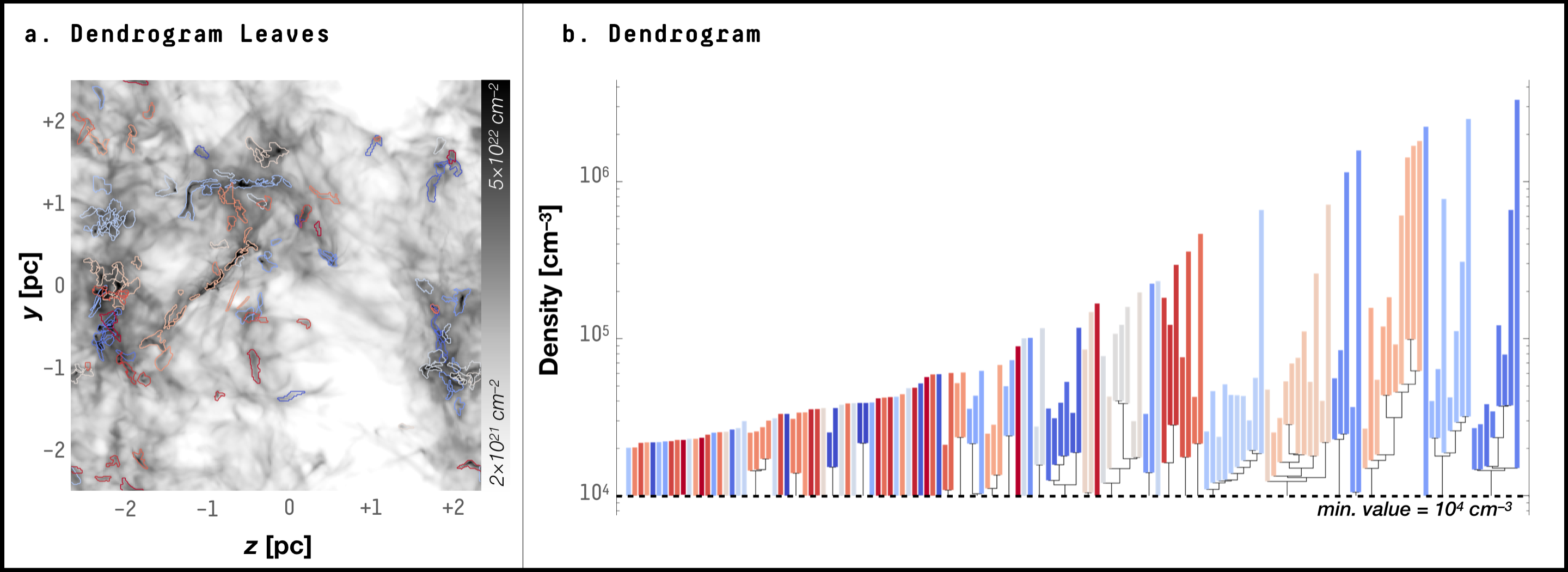
We identify cores in each snapshot of the MHD simulation described in §2.1 using the dendrogram algorithm (Rosolowsky et al. 2008b; Goodman et al. 2009, hierarchical structure extraction algorithm; ). Dendrogram-based extraction algorithms (hereafter the dendrogram, for simplicity) efficiently identify density structures in star-forming regions in both simulations (Hopkins 2012; Burkhart et al. 2013; Koch et al. 2017, e.g.,) and observations (Goodman et al. 2009; Lee et al. 2014; Seo et al. 2015, e.g.,). For each snapshot, we apply the dendrogram on the density distribution in the 3-d space. We construct the dendrogram to find structures with densities above 104 cm-3, which is characteristic of the densities traced by NH3. To guarantee enough sampling points for the analysis of density and velocity distributions, a structure must have a volume of at least 100 voxels (0.02 pc in linear size) to be included in the dendrogram. To avoid the inclusion of insignificant local density fluctuations, a structure must also have a difference of 104 cm-3 in density between its peak and the node where it merges onto the tree.33 3 These setup parameters translate to min_value of 104 cm-3, min_delta of 104 cm-3 and min_npix of 100 in astrodendro A tree is a full dendrogram representation of hierarchical structures.. We identify a total of 3,538 structures over a time span of years, with a nominal time resolution of years. Note that we use the dendrogram only to identify independent density structures and locate their peaks. We do not limit our following analysis of the density distribution to only the density range above 104 cm-3 (see §3.2 for details), and we only use the dendrogram boundary to avoid confusion with a neighboring core. See Fig. 2 for an example of the independent structures identified using the dendrogram algorithm.
To follow the identified cores as they move and evolve in the simulated box, we devise a tracking procedure by first identifying the density peaks within independent structures, leaves, in the dendrogram of each snapshot. The tracking procedure then uses the velocity at the position of the density peak to predict where the density peak is expected to be in the previous and following snapshots. If the expected position falls within the boundary of a dendrogram leaf, the tracking procedure links the original structure with the leaf in the previous or following snapshot. This tracking procedure is similar to but less detailed than the one deployed and analyzed by Smullen et al. 2020, in which the overlap in various physical quantities and statistical measurements are examined when dendrogram structures in different snapshots are compared. Our tracking procedure then repeats the process by going through the total of 3,627 independent structures of the dendrograms derived for the snapshots used in this study.
We find that 3,538 out of 3,627 structures (97%) are connected to 450 tracks, which link cores identified in two or more snapshots. As Smullen et al. 2020 have pointed out, the robustness of the identification using the dendrogram algorithm is subject to uncertainties due to the stochastic fluctuation in the density distribution over time, even when the dendrograms are derived using the same set of input parameters. We try to avoid the issue of density fluctuations affecting the robustness of dendrogram tracking by excluding structures that are not connected to any of the tracks. This is equivalent to removing structures that are captured by a dendrogram only in a certain snapshot but not the preceding nor the subsequent ones (separated by 1.5104 yr; see above).
Of the 450 tracks, 146 (32%) end after merging with another track such that they no longer have a unique, distinct peak that can be identified. Since we are particularly interested in the evolution of cores from formation to either star formation or dispersal, we limit our evolutionary study to consider only the 304 main tracks, i.e., we exclude short-lived over-densities that merge with larger ones. We exclude only the minor structure in the merger for the following reasons. If the peak of a structure disappears due to a merger, its track terminates abruptly after a significant jump in the core properties (because the track is matched to a new peak/object). Neglecting these histories allows a cleaner analysis and clearer visualization of evolutionary trends. We, however, include the dominant structure in the analysis since the merger does not abruptly affect the inner profiles near the peak or the bulk properties, which are generally derived from a compact region around the peak.
The average lifetime of the 304 tracks is years. 21 tracks span the entire simulation calculation of yr. 15 out of the remaining 304 tracks (5%) are connected to at least one structure with a sink particle of a mass 0.1 M⊙; several of these are matched to two or three sink particles. 167 of 304 (55% or % of 450) cores disperse, i.e., their track ends before forming a sink particle, merging with another track or reaching the last snapshot. Generally, this occurs if the core size or density maximum falls below the dendrogram structure requirement.
3.2 Constructing Physical Properties of Identified Cores

In order to analyze the core evolution and compare with observations, we must define a set of fundamental core properties that represent essential characteristics of each core. This step serves as an initial layer of dimensionality reduction, where we reduce the high-dimensional simulation phase space of gas position (), velocity (), and density () to a smaller set of parameters that more directly represents each core and can readily be compared with observations.
We first describe each core as a vector of physical properties that contains the radial density and velocity dispersion profiles (50 radial measurements for each), exponent of a power-law fit to the density profile, and bulk core properties, including radius, mass, velocity dispersion, and ratio of kinetic energy to gravitational energy. We adopt this particular set of bulk properties because they correspond to the set of physical properties previously derived from the observed dense cores in our observational samples (see §2.2). Here, we describe how we derive each of these parameters.
We take the following steps to derive radial profiles. First, we draw a series of constant density isosurfaces, each at a number density . Since the isosurfaces may take any shape as dictated by the gas distribution, we make no assumption about the geometry of the cores. We use 51 density values uniformly spaced on a logarithmic scale from = 102.5 cm-3 to 105.5 cm-3. As Fig. 3 shows, these densities sample the underlying probability density function (PDF) of gas density well. Each isosurface is then converted to an equivalent radius by finding the radius that would construct a sphere that has the same volume as the volume enclosed by the isosurface, i.e., .44 4 We note this definition is the 3-d equivalent of the effective radius that is often derived in observations of clouds and cores (Rosolowsky & Leroy 2006). The radial density profile, , is then constructed from the series of densities, , that define the isosurfaces and the corresponding equivalent radii, . For the velocity dispersion profile, we calculate the velocity dispersion of material enclosed within each isosurface, , and similarly construct the profile of velocity dispersion, , from and . Note that the profile represents the 3-d turbulent velocity dispersion and does not include the thermal sound speed. The structure boundaries defined by the dendrogram are only used to avoid confusion with another core. We stop the construction of profiles when the volume enclosed by the isosurface overlaps with the dendrogram boundary of another core. This occurs mostly when the core has a sibling, i.e., a nearby leaf that has the same density minimum and shares the same parent branch in the dendrogram. For a core that does not have a sibling (Rosolowsky et al. 2008b, the trunk-leaves—independent structures at the bottom level;), the extent of the radial profile is not limited by the dendrogram structure boundary (see §3.1). This method does not involve spherical averaging and can produce radial profiles for structures with different shapes in a reliable and consistent way.
We use the 1-d profiles to derive the rest of the core properties. In order to better compare with the observations described in §2.2, we define the boundary such that the core radius, , is the FWHM of the density profile. This definition is similar to that adopted by the getsources algorithm, which is commonly used to define observed structures. While this does not allow a true apples-to-apples comparison, using the FWHM as the core boundary produces simulated core with masses, sizes and velocity dispersions comparable to the those of observed cores (see §4.5). We derive the core mass, , by integrating the density profile to obtain the mass enclosed by . Since observations do not include protostellar information in core estimates, we exclude the sink mass in the calculation of and all the other core properties. For the total velocity dispersion of the core, we adopt the observational definition in Equation 1. Here, and is the sound speed for a 10 K molecular gas. We define the radius of coherence, , as the radius where the velocity dispersion falls below the sound speed: . We obtain the density power-law index by performing a least squares fit on the density profile for pc.
Using the mass, the size and the velocity dispersion, we derive the kinetic energy and the gravitational potential energy. For the purpose of later observational comparison (see §4.5), we adopt the expressions from Chen et al. 2019a, where the kinetic energy is
| (2) |
and the gravitational energy is
| (3) |
The latter expression assumes the cores have a uniform density distribution. Cores with a density profile will have an actual gravitational energy a factor of times larger than that expressed in Equation 3 (Pattle et al. 2015).
To evaluate the impact of the choice of core definition on our analysis, we also adopt a fixed density contour to define core boundaries. We present this analysis in Appendix D. There we demonstrate that while the quantitative distribution of core properties depends on core definition, the qualitative determination of phases and our conclusions are reasonably robust to the core definition.
After deriving the properties for each core, we remove duplicate information by reducing the number of profile data points that contribute to the final data vector. We describe our procedure in Appendix A. This effectively reduces the weight of the profiles in the later analysis, so that the bulk and profile information is considered more equally. This process reduces the 100 profile values to 22.
Finally, we assemble a data matrix composed of physical property measurements for each of the structures identified by the method of §3.1.
3.3 Core Clustering Methodologies
Our goal is to identify groupings of the 3,538 cores in order to differentiate evolutionary behavior based on physical properties. Because our data arise from discrete snapshots of the continuous process of an MHD simulation (§2.1) we have reason to suspect the boundaries separating (defining) each phase are less crisp than those arising from a truly discrete process. This complicates the clustering task, whose goal is delineation of such boundaries. To aid cluster saliency while still acknowledging the fuzziness of our data groupings we employ two approaches from unsupervised machine learning: (1) we learn prototype representations of our data and then (2) create a soft partitioning of these prototypes based on the Fuzzy -means algorithm. The benefits of this two-pronged approach are discussed in the next two sections.
3.3.1 Learning Prototypes of Core Properties
Prototype-based methods in machine learning (Biehl et al. 2016) apply common machine learning tasks (e.g., clustering or classification) to intelligently formed representations of the data called prototypes (instead of the data themselves). That is, from data observations we learn prototypes . The prototypes arise from the codebook of a vector quantizer (Gray 1984) trained on and benefit the learning task by simultaneously reducing sample size (typically ) and decreasing noise (the process of quantizing an by its best representative separates the signal and noise components of ). While classical -means (MacQueen et al. 1967) with a large number of centroids is a common method for obtaining prototypes, in this work we obtain prototypes of our cores from the Batch Neural Gas algorithm (Cottrell et al. 2006, extended from Martinetz & Schulten 1991) trained on the core properties. Neural vector quantizers (Neural Gas, as well as the Self-Organizing Map, see Kohonen et al. 2001) benefit from a cooperative element during their training process, rendering them less sensitive to the initialization issues common for -means (Cottrell et al. 2006). No theory currently exists for selecting an optimal number of prototypes: there should be enough to fully capture intricacies of the data distribution, but not so many that the vector quantizer approaches an identity mapping. Often, analyses adopt empirical rules of thumb from related areas such as kernel density estimation that suggest . Here we select the optimal number via an iterative process: we start with M=100 and learn. If all prototypes are utilized, i.e., there are no dead prototypes with empty receptive fields, we increase by 50 and repeat, stopping once the set contains at least one dead prototype. This process yielded = 249 prototypes (1 dead prototype was removed after the last iteration) for the 3,538 cores; because we find a similar number of clusters and set of cluster properties for , we conclude that our analysis does not strongly depend on the number of prototypes within a factor of 2.
Beyond sample size and noise reduction, vector quantization provides a unique prototype similarity measure which we consult for intelligent parameterization of part of our analysis (see Appendix C for details). For completeness we also compared our results with those derived from a more basic principle component analysis (PCA) and from a self-organizing map (SOM) of the core data. We find that both these approaches return qualitatively similar cluster organization and cluster assignments. We present the Neural Gas prototype analysis here, since it provides the best combination of group separation and simplicity.
3.3.2 Fuzzy c-means Clustering
Once learned, the core prototypes are clustered by a user-selected method and the cores themselves inherit the cluster label of their best representative. The continuous nature of our data (§3.3) suggests we should expect some cluster overlap; to account for this, we choose a soft partitioning of the core prototypes by the Fuzzy -means algorithm (or FCM, Bezdek et al. 1984). Typical hard partitioning schemes assume well separated data clusters and, consequently, assign data to a single cluster. Soft partitionings instead report a membership strength representing the degree to which datum belongs to cluster . By convention, , , where denotes a datum’s strong membership in cluster . Importantly, the graded information contained in influences the formation of cluster centers in soft partitioning algorithms. For completeness, we note that hard partitionings are a special case of soft partitionings where the are constrained to the set . From the analysis of Appendix B, FCM applied to our core prototypes suggests clusters (evolutionary phases) exist in the simulated core sample. To mitigate initialization issues, the clusterings reported in this work are optimal, i.e., have lowest within-group error over 1,000 different randomly initialized runs of FCM.
3.4 Visualization with UMAP
Note that the evolutionary tracks described in §3.1 were not used by FCM during the clustering procedure; therefore, the resulting partitioning produces clusters of cores with similar physical properties. Our goal is to uncover a relationship between these groupings and a core’s evolution. To this end we employ a 2-d visualization of core prototypes via the UMAP algorithm (McInnes et al. 2018), which serves two purposes: 1) it allows inspection of the integrity of the three FCM-identified clusters and 2) provides an organized space upon which to view the core tracks. Figure 4 shows the UMAP visualization of the prototype data and the resulting three clusters identified as described in §3.3.2. UMAP has gained popularity relative to other common approaches for dimensionality reduction, such as t-SNE, due to its visualization quality, ability to retain high-d structure in the lower-d projection and calculation speed. The data visualizations (e.g., Figures 4 and 6), along with associated group-wise statistics of Figure 7 and Table 1 underpin the evolutionary interpretation of our clustering, as discussed in §4.2. An overview of UMAP and an explanation of the parameters used in this work can be found in Appendix C.

4 Results
| Core Classification | (M⊙) | (pc) | (pc) | p | (km s-1) | (km s-1) | / | (%) | (pc) | |
|---|---|---|---|---|---|---|---|---|---|---|
| Phase I (Turbulent) | 1221 | 0.3 | 0.034 | 0.012 | -0.9 | 0.27 | 0.6 | 6.3 | 0.82 | 0.17 |
| Phase II (Coherent) | 1317 | 0.4 | 0.040 | 0.029 | -0.9 | 0.23 | 0.4 | 3.2 | 0.0 | 0.18 |
| Phase III (Protostellar) | 1000 | 0.3 | 0.023 | 0.008 | -1.2 | 0.26 | 0.6 | 2.9 | 22.9 | 0.13 |
| All | 3538 | 0.3 | 0.032 | 0.016 | -0.9 | 0.25 | 0.5 | 3.9 | 6.8 | 0.16 |
4.1 Properties of Core Phases
Table 1 summarizes the simulation core properties for all 3,538 cores and for cores classified in each of the phases. While the core masses are similar across all phases, clear differences appear in the other median properties. Phase I and Phase II cores have similar masses, sizes and density indices, however Phase II cores contain a large subregion with a subsonic non-thermal velocity dispersion, i.e., a region of coherence (Pineda et al. 2015; Chen et al. 2019a). Consequently, we term Phase II the coherent phase. Phase II cores also have a slightly lower overall non-thermal dispersion and a lower bulk velocity. Phase III cores have the steepest density index () and the lowest ratio of kinetic to gravitational energy (). Since our calculation for the gravitational potential assumes a uniform potential these virial parameters are likely over-estimated by a factor of 1.7, which means that most of the Phase III cores are gravitationally bound. We also find % of these contain sink particles (compared to % and 0% of Phase I and II cores, respectively). Therefore, we term Phase III the prestellar/protostellar phase. Of the three phases, Phase I has the highest ratio of kinetic to gravitational energy. Consequently, we refer to Phase I as the turbulent phase. In order for cores in this phase to form stars they must either gain significant mass or reduce their gas velocity dispersion (possibly by passing through Phase II).
Cores almost always belong to Phase III after forming protostars (see Figure 4), so it can be loosely considered the last phase. However, there is no one evolutionary order between I, II and III and not all cores that belong to Phase III at a given time go on to form protostars (see §4.2 for more discussion). Cores may form in any phase and take a variety of different routes to evolve through the parameter space until they become protostellar or disperse as we discuss in detail in §4.2.
Figure 5 shows a column density map with the identified structures colored by their phase. Most of the Phase III cores are located within large filaments, which is also where most of the protostars reside. Many of the Phase I and II structures are associated with shocks and/or more isolated filamentary features. They also tend to be larger and have lower column densities, which is consistent with being gravitationally unbound.
Figure 6 shows the distributions of core radii, masses, velocity dispersion, virial ratio (ratio of kinetic to gravitational energy), density index and size of the coherent region. The clusters do not divide cleanly across any of these properties, but there is evidence of property gradients. For example, Figure 6a shows core sizes transition from large to small from bottom to top. The core mass distribution exhibits similar structure as shown in Figure 6b, with the lowest mass cores appearing at the top of Phase I and Phase III. Similarly, Figure 6c shows a strong vertical gradient in velocity dispersion, which is echoed in the distribution of virial ratios shown in Figure 6f. There are two distinct regions of high virial ratio: one appears in Phase I, where cores seem to be genuinely unbound due to high levels of turbulence, and the other occurs in the topmost corner of Phase III, where the high dispersion is produced by infall. The prototypes within the lower region of Phase III have the lowest virial ratios, suggesting that cores are becoming bound as they approach the stage of gravitational collapse. Unlike the others the density index exhibits stronger horizontal gradients, with steeper profiles on the very right and left, while flatter profiles appear in the center. Figure 6d shows the cleanest and most monotonic trend across phases of all six properties: there is a strong vertical gradient in the size of the coherent region, with the most coherent cores located at the bottom left of the UMAP (Phase II) and cores with no coherent region at the top right (Phase III).

Fig. 7 displays the density and non-thermal velocity dispersion profiles for each of the clusters (left panels) and the distributions for radius, total velocity dispersion, mass and virial ratio (center and right panels). With the exception of mass, the profiles and properties exhibit distinct differences for the three phases. Phase I and II have significant overlap in several of the properties but are distinguished by the velocity dispersion: Phase I cores are more turbulent at all radii, while Phase II cores have velocity dispersion profiles that dip to sub-sonic values near the core center, i.e., they have an internal coherent region. This difference in velocity dispersion is also reflected by the virial ratio, which tends to be higher for Phase I cores. Phase III cores exhibit noticeably steeper density profiles with a higher central density. Meanwhile, the velocity dispersion of Phase III cores is typically supersonic for all radii with velocity dispersion flattening or increasing near the center. This feature, together with the steeper density profile, is consistent with gravitational infall dominating the internal kinematics of the core and the incipient formation of protostars. For this reason, Phase III cores are also more compact on average because the FWHM corresponds to a smaller region (see Appendix D).
4.2 Core Evolution
In this section we use the core histories and cluster assignments to explore how cores evolve through the cluster phase space.
We first calculate how long cores typically spend in each of the three phases. By averaging over the time cores spend visiting each phase, we derive an effective phase lifetime; cores that never visit a phase are not included in its time average. We estimate typical lifetimes of 1.00.1105 yr, 1.30.2105 yr, and 1.80.3105 yr for Phase I, II and III, respectively. We find that a core evolving into Phase III spends significantly longer there. For example, cores that eventually form protostars spend 0.60.3105 yr visiting Phase I and/or II and 5.00.4105 yr in Phase III. This is because star-forming cores remain in Phase III after becoming protostellar and also because the lifetimes of cores that visit Phase III tend to be systematically longer. The lifetime of Phase I is the shortest, which is consistent with most of the cores being unbound.
Next we investigate the trajectories of cores through the phase space. Figure 8 shows tracks for three different sets of core histories: short-lived tracks, which connect cores that appear only in two snapshots, long-lived tracks, in which the cores persist for all simulation snapshots but do not form stars, and sink tracks, which represent the evolution of cores that eventually become protostellar. Arrows represent the aggregate direction of movement for all cores passing through the associated prototype, constructed as a quadratic Bézier curve with control points set by the median incoming direction (arrow tail), the prototype itself, and the median outgoing direction (arrow head). The unit vectors describing the incoming/outgoing control points are further scaled by the proportion of incoming/outgoing tracks transiting through each prototype. Thus, higher arrow curvature indicates more misalignment between the median incoming and outgoing track directions, and an asymmetry in arrow length (relative to the arrow’s middle elbow) indicates areas of core birth (longer outgoing head) or dissipation (longer incoming tail).
As UMAP is a highly non-linear manifold projection, some of the strong curvature observed in Figure 8 is to be expected. For example, prototypes representing sink particles appear in a circular region in the top right as shown by Figure 8c, and the arrows connecting neighboring prototypes naturally possess curvature to follow the circular structure in an organized manner. However, in more linear regions of the embedding, curvature indicates track reversal of the incoming / outgoing movement of a prototype’s typical core. The strongest examples of such core meandering occur in the long lived tracks of Fig. 8b, indicating that these tracks bounce from one prototype to another (i.e., they migrate between different set of physical characteristics) continuously due to small changes in their properties. One fundamental implication of this figure is that there is no one evolutionary path for cores.
The short-lived tracks represent relatively transient cores that quickly disperse. These tracks inhabit the top left part of the phase space, lying almost entirely within Phase I and II. Many of the arrows point along the edge or outwards as if they are exiting the UMAP boundaries. These cores disappear because their densities and/or sizes fall below the threshold of detection by our dendrogram algorithm, which is consistent with the small masses and sizes of cores in this region of the parameter space (e.g., compare Fig. 8a and Fig. 6ab).
The long-lived tracks inhabit the middle of the UMAP, spanning parts of Phase I, II and III. They appear to complement the short-lived tracks, since their motion is concentrated in the right half of Phase I and the bottom of Phase II. Their longevity suggests that they have achieved some degree of equilibrium, and inspection of many of these cores indicates that they become coherent, moving into Phase II, and remain there for much of their lifetime. This is illustrated by the shortness of the arrows, which indicate that many cores mapped to prototypes in the middle of Phase I and II do not undergo rapid or significant changes in their properties between snapshots. The general impression is that this subset of cores evolve more gradually between phases. Since there is no preferred phase where cores start, the initial position is not predictive of the longevity or the direction of evolution.
The behavior of the cores following sink tracks is potentially the most interesting, since these cores are the subset that eventually form stars. The arrow directions generally point towards the upper right, suggesting that these cores move rightwards and upwards in the parameter space as they evolve. Cores with sink particles lie almost exclusively in the top right corner of Phase III, which is consistent with the apparent trajectory of these cores. Prestellar cores, i.e., those that later go on to form stars, mostly ( 9 of 15) start in Phase II. These cores become protostellar while in Phase III, in a region of the parameter space in which the virial ratio is small, and remain in Phase III for the remainder of their evolution. Despite spending most of their evolution in Phase III, 73% of cores that eventually become protostellar spend time in another Phase: on average 0.60.3105 yr visiting Phase I and/or II and 5.00.4105 yr in Phase III. Note that prototype locations in Phase III can also host some short and long-lived cores, and thus the initial core properties and phase space location are not entirely predictive of the eventual evolution.
Finally, in Figure 9 we synthesize the evolutionary information by coloring the UMAP not by cluster membership but by the outcome of the evolution of the cores passing through each prototype. Here we denote four states: cores that are protostellar (red), cores that are prestellar and will eventually become protostellar (orange), cores that disperse (blue) and cores that neither disperse nor form protostars by the end of the simulation (green). Many cores comprising the last class have reached a quasi-equilibrium state due to magnetic, turbulent and thermal pressure support, and they are represented by the long-lived tracks. Figure 9c shows that prototypes on the left represent predominantly dispersing cores, while pre/protostellar cores are almost exclusively mapped to prototypes on the right.
Note that the core histories are not included in the information used to perform the clustering, and thus represent an independent view of how the clusters relate to one another. In many cases, the clustering appears to intuit some of the evolutionary movement, since related prototypes, e.g., those representing star-forming cores, are confined to specific regions of the visualization. However, Figure 9 shows the evolution is not cleanly represented by particular properties, which show a vertical separation. While cores assigned to Phase I and Phase II have distinct properties, these properties only partially predict whether the cores will disperse, persist or form stars (see §4.3 for further discussion of evolutionary rates). Disorder in the UMAP is produced by the stochastic nature of star formation: core properties vary as a function of the environment, formation and accretion history.


4.3 Survival Rates & Lifetimes
In §4.2, we show that evolutionary tracks exist that connect three populations of cores with different physical properties. A closer examination of the survival rates, defined as the fraction of cores remaining in a given phase, reveals that cores classified in the same phase can follow distinctly different evolutionary paths. Figure 10 shows the percentages of cores in a given phase that stay in that phase, eventually move to another phase and/or disperse. For example, if a core starts in Phase I, moves into Phase II, and then moves to Phase III before finally dispersing, it will be counted in the statistics of cores that are born in Phase I (54%), move from I to II (41%), move from II to III (13%) and then disperse from III (15%). If that core belongs to the subset of cores that persist or eventually form stars Figure 10b shows that for this path only 22% are born in Phase I, 43% move from I to II and 47% move from II to III. Stated another way, this figure shows the transition probabilities for a core observed in a given phase. For example, if a core is currently observed in Phase III, the probabilities of either transitioning next to I or II or to dispersing from Phase III are shown in the figure. We include 95% confidence intervals to give a sense of the uncertainties based on the core statistics.
We find that all cores have a relatively high probability of phase transition: 854% either move to another phase, disperse, or both, during the simulation, while 556% of cores belong to two or more phases during their evolution. Phase I cores are most transient with only % chance that a core in that phase remains there for the remainder of its life. Approximately a quarter of the cores disperse from each phase, with cores in Phase II having the lowest survival rate and Phase III cores having the highest (only % cores disperse from this phase).
Figure 10a shows there is a lot of movement between Phase I and II. While it is most likely that a Phase I core transitions into Phase II %, there is a nearly equal probability, %, of a Phase II core transitioning to Phase I ( see also Fig. 8). Phase III cores are most likely to remain in their current phase, in part because 23% of Phase III cores are protostellar. Phase III cores that do leave are more likely to move into Phase I (%) than into Phase II (%). This core subset has a significant amount of initial turbulence: they can’t immediately collapse because they are not bound by gravity. Figure 10 shows that while most cores are born into Phase I (54%), the majority of cores that persist or form stars, i.e., the ones that don’t disperse, begin in Phase II (64%). In either case very few cores start in Phase III.
Note that while the phases can be described by average properties, there is a range of properties within each phase. This is also illustrated by Figure 11, which shows the distribution of prototype visiting times, i.e., how long a typical core is matched to a given prototype. For example, cores in the upper right of Phase III are not likely to change phase or disperse because most already host stars. This is also reflected in the longer time periods a core matches a given prototype in this region. Interestingly, Figure 11 shows there is another grouping of long-lived prototypes towards the bottom of Phase II. Inspection of Figure 7 indicates that these are moderately-sized cores that are marginally bound and quiescent, i.e., these are coherent cores that have reached a quasi-equilibrium state. In contrast, the prototypes in Phase I tend to have the shortest lifetimes (3.80.5104 yr vs. 5.20.6104 yr in Phase II and 5.90.7104 yr in Phase III ), indicating that the properties of Phase I cores change relatively quickly.

4.4 Core Properties
In this section we present an analysis of the physical properties derived using the core profiles constructed from the dendrogram-identified hierarchy.
Fig. 12a shows mass as a function of size for cores in each of the three phases. The phases generally fall along a power-law relation where the Phase III cores, which are often protostellar, are offset to a higher mass at a given radius. The protostellar cores are more centrally peaked such that the FWHM core definition returns more compact structures. A power-law fit to the mass-size distribution of cores belonging in all three phases gives a power-law index of 1.5. A fit to only the Phase I and Phase II cores returns a power-law index of , as expected from Larson’s relations (Larson 1981). Appendix D shows that the power-law index is sensitive to the core definition, however.
Fig. 12b shows non-thermal velocity dispersion, , as a function of size for structures in each of the three phases. As expected from the velocity dispersion profiles examined in §4.2, Phase I and Phase III cores generally have larger velocity dispersions than Phase II structures, which generally have subsonic dispersions. Protostellar cores have the largest velocity dispersions due to gravitational infall. Since the simulations neglect mass-loss due to protostellar outflows, the sink particles are over-massive (Smullen et al. 2020) and the degree of infall, and hence the non-thermal component, is likely over-estimated.

Fig. 13 shows gravitational energy versus kinetic energy for cores in the three phases. Such a comparison, conventionally known as a virial analysis, provides a first-order estimate of the gravitational boundedness of a structure. A virial analysis may sometimes include other terms such as the magnetic energy and the surface pressure term (Ward-Thompson et al. 2006; Pattle et al. 2015; Chen et al. 2019a, see). Since the core mass does not include the sink mass, we note the gravitational binding energy of the protostellar core is underestimated. We find that there is no clear separation in the distribution of kinetic and gravitational energies between Phases. In contrast, see the analysis in Appendix D, which also shows that these properties are sensitive to the core definition. However, there appear to be more Phase III cores with high gravitational and kinetic energy that are more gravitationally bound, consistent with the star-forming activities found within many of them. Phase I and II cores are almost all below the equilibrium line and are unbound when considering only thermal, gravitational and kinetic energy. Recall that our definition for the gravitational energy in Equation 3 assumed a uniform density; we see here this description is more accurate for Phase I and Phase II cores, which have a relatively flat density profile.

| Disperse | Persist | Pre/Protostellar | |||||
|---|---|---|---|---|---|---|---|
| Region | (total) | % | % | % | |||
| Ophiuchus | 30 | 6 | 219% | 4 | 219% | 20 | 5814% |
| Orion | 43 | 3 | 195% | 14 | 268% | 26 | 5512% |
| Cepheus | 22 | 0 | 72% | 2 | 1310% | 20 | 8010% |
| Perseus | 33 | 2 | 176% | 12 | 3111% | 19 | 5213% |
| Droplets | 23 | 18 | 5412% | 4 | 3911% | 1 | 77 |
| Taurus | 8 | 2 | 2127% | 6 | 6524% | 0 | 148% |
| All | 159 | 31 | 224% | 42 | 284% | 86 | 506% |
4.5 Classification of Observations
In this section we compare the observed cores with the simulated cores by using their properties to match them to prototypes and project them into the UMAP parameter space. Each observed core inherits coordinates in the UMAP plane from their most representative prototype among those trained on our simulated cores according to §3.3.1. Recall (§3.2) that each prototype represents 28 different physical core properties, with the radial density and velocity dispersion profiles comprising 22 of the 28. As this information is missing from the observed cores, we have mapped observations to prototypes based solely on their radius, mass, velocity dispersion, and virial ratio by excluding the radial profiles learned by the neural gas prototypes during quantization. The size of the cores identified by Chen et al. 2019a is defined by construction to be the size of the coherent region, so we use the coherent radius instead of the radius to project this sample into the UMAP. We acknowledge that the neural gas algorithm may well have learned to represent this reduced four-dimensional space differently (i.e., produced a different set of prototypes), but any re-training would necessitate a separate clustering (§3.3.2) and produce a different UMAP embedding (§3.4).
We note that 33 (of 159) observed cores have a property that falls slightly outside the range of the properties of the simulated cores. The Cepheus cores, which adopt a different core definition and appear the most bound of all the core catalogs, have the most discrepancy. However, since these differences are within the observational uncertainties, we do not exclude them from our comparison. Inspection of their phases and location in UMAP space indicates that their classification is still consistent with the expectation given their general properties.
Figure 14 shows the observed cores are mapped to locations across the UMAP space. In some cases, multiple cores in different regions are mapped to the same prototype, as in the top right, while other prototypes have no observational match. The droplets identified by Chen et al. 2019a are mostly mapped to prototypes in Phase II. This is consistent with droplets being quiescent, coherent structures by definition. The cores observed in Taurus (Kerr et al. 2019) are likewise mostly mapped to prototypes that are classified as Phase II.
In contrast, few cores in Perseus, Ophiuchus and Orion (Kirk et al. 2017; Kerr et al. 2019) match prototypes in Phase II. These cores predominantly belong to Phase I or III, and they are instead located in regions of the parameter space characterized by high velocity dispersions and high virial ratios (top of the UMAP) as shown in Figure 6. The Perseus and Ophiuchus cores were selected to be starless by construction, and their correspondence with prototypes in the top right – where the simulated protostellar cores lie – may either mean they are prestellar and close to forming stars or that their properties are similar because they belong to more clustered environments, which is also true of the simulated protostellar cores (see Table 1). The Cepheus cores from Keown et al. 2017 are all mapped to a few prototypes in the top right of Phase III, a region of the parameter space containing mostly prestellar, bound simulated cores (see Fig. 6).
To be more quantitative, we employ the simulated core distribution to predict the evolution of the observed cores. Table 2 lists the predicted probabilities of future evolution for cores observed in each star-forming region. To obtain these predictions, we mapped the observations to their most similar simulated core using the available subset of bulk properties (radius, velocity dispersion, mass, and virial ratio). UMAP coordinates for each observation were inherited from its nearest simulated neighbor, and a Bayesian classification probability was obtained using the kernel density estimates of each evolutionary stage visible in Figure 9b. In most regions about 20% of cores are expected to disperse while % are expected to eventually form stars. The droplets have the highest rate of expected dispersal (%), while the Cepheus cores have the lowest (%). % of the cores in Taurus are expected to ‘persist’, i.e., they are likely long-lived quasi-equilibrium structures. This is consistent with Taurus being a quiescent region where the star-formation is most distributed. Overall, at least % of the observed cores are expected to disperse, while at least half are likely to form stars in the near term.
Figures 15 and 16 compare the properties of the individual observed cores to the simulated cores. As shown by the prototype comparison in Figure 14, there is good agreement between properties of observed and simulated cores. In the 2-d parameter spaces of physical properties there is significant overlap between the phases, so it is not always clear which phase an observed core belongs to, for example, on the basis of velocity dispersion and radius, alone. However, we can still infer some general trends by inspecting the distribution of observed core properties.
Figure 15a displays total velocity dispersion versus effective radius for the three phases and the observed cores. Most of the droplets lie in the Phase II region, which has a lower total velocity dispersion and where the total is dominated by the thermal component. The cores in the warmer and more clustered regions – Orion, Perseus and Ophiuchus – lie predominantly in the Phase I and Phase III regions, where the velocity dispersions are higher. By construction most of these cores are starless and relatively few fall into the high-dispersion, compact size region (upper-right Phase III quadrant) where the simulated protostellar cores lie. The Taurus and Cepheus cores generally fall within the Phase I and II regions. As we discussed in §4.3 the simulations predict a high level of core dispersal, and the location of the observed starless cores in phase space is not predictive of whether a core will definitively go on to form stars (although cores found in the middle part of Phase III are more likely to be or become star-forming).
Figure 15b shows gravitational energy versus kinetic energy for the three phases and the observed cores. There is likewise a high degree of overlap between the phases, which suggests that the virial ratio cannot uniquely determine the core phase. In this space, there is also good agreement between the simulated and observed cores with most of both appearing to be unbound. However, a subset of the observed cores have high gravitational energies and these extend outside the simulation parameter space. Nearly all of these are cores in Cepheus, which were defined using the dendrogram leaf boundary and thus are systematically larger than cores in the other clouds. Our analysis in Appendix D suggests that in fact the low virial ratios may be partially due to the core definition.
Figure 16 shows core mass versus coherent region size for the three phases and cores from Chen et al. 2019a. This data is only available for the droplet population, which are explicitly identified and defined by the extent of the coherent region. The droplets fall almost entirely within the simulated Phase II region; two have significantly higher masses and sizes. While there is some overlap between the three phases, the resolution of the observations appears to limit the minimum detected size of the internal coherent subregion, such that any detected sizable coherent region uniquely identifies cores as belonging to Phase II. The simulation phase distributions suggest that other observed cores likely contain coherent regions with sizes below the observational resolution ( pc).
5 Discussion
5.1 Predicting Core Evolution
Based on the results presented in §4, we propose an evolutionary scenario where cores inhabit three distinct phases. Cores in these three phases bear characteristically different physical properties. In summary, cores are born as turbulent density structures that, depending on their initial size and virial ratio, may belong to any of the three phases. A subset of the smallest and most unbound cores quickly disperse (e.g., as Fig. 8a). Cores that are initially bound and classified as Phase III may begin collapse and form protostars without passing through other phases (see Fig. 8c). In contrast, cores that are marginally bound and/or pressure confined (depending on core definition, see Appendix D) but not sufficiently massive to collapse likely undergo a phase of turbulent decay, developing a significant central coherent region, and evolving into Phase II. Such cores may transition between Phases I, II and III depending on their local environments and how they accrete material (Burkert & Bodenheimer 2000; Hennebelle & Chabrier 2009; Hopkins 2013; Padoan et al. 2020, e.g., as described by).
Due to the turbulent nature of the core environment, we find that core characteristics are non-deterministic. Cores in all three phases may disperse (Fig. 10, see also Smullen et al. 2020). This suggests that the location of an observed core in the parameter space does not uniquely determine whether it will survive or become protostellar. Cores with significant coherent regions are more likely to live longer but are also not guaranteed to form stars at a later time ( e.g., Table 2). This suggests that many observed starless cores may not in fact go on to form stars. For example, our results suggest that low-mass cores with initially high virial ratios, such as a subset of Orion and Ophiuchus cores that appear towards the top of Phase I (see Fig.15) have a high likelihood of dissipation within years.
The exact percentages for the survival rates likely depend on the degree of clustering and cloud physical conditions (Guszejnov et al. 2022, e.g.,). However, the fact that some cores not bound by self-gravity continue to evolve and may eventually become prestellar/protostellar is consistent with the substantial number of observed unbound cores. Chen et al. 2019a found that (Phase II) coherent cores, not bound by self-gravity, are instead confined by turbulent motions of the ambient gas. Similarly, Orion and Ophiuchus contain a large number of unbound cores, which can be explained by a significant confining pressure (Kirk et al. 2017; Kerr et al. 2019). This confinement, provided by the turbulent pressure of the ambient gas, helps explain why many apparently unbound cores persist and some eventually become protostellar (e.g., Fig 8bc). Our analysis suggests that the degree of unboundedness may be due in part to the fiducial core definition, which focuses on an inner compact portion of the core and misses a substantial part of the core mass (see Appendix D). However, we caution that even if confining pressure helps to explain the existence of the large number of such structures, our results imply that many of these will not go on to form stars.
Cores inhabiting Phase III have the highest likelihood both of persisting (%) and of being protostellar (%). This suggests the subset of observed starless cores in Ophiuchus, Orion and Perseus mapped to Phase III prototypes will become protostellar. Based on our tracks this may occur within years, although the timescale for the evolution is difficult to constrain from the placement within the UMAP alone.

Overall, cores appear to transition smoothly between phases as evinced by the significant amount of time cores often spend in one prototype and one phase before moving to another (e.g., Fig 11) and the concentration of tracks in limited parts of the parameter space (e.g., Fig 8). As discussed above, the appearance and growth of coherent regions appears to be gradual, and a core remains not bound by self-gravity in parts of Phase II. On the other hand, the transition between Phase II and Phase III or Phase I and Phase III corresponds to a shrinking or complete disappearance of the central coherent region (Fig. 6). However, we note that there is a certain degree of overlap and that some of the Phase III cores still contain coherent regions (Fig. 6 and Fig. 15). An observational example is the star-forming coherent core in the B5 region in Perseus identified by Pineda et al. 2010. This coherent core is associated with a known protostar and contains at least three other starless substructures (Pineda et al. 2015). Pineda et al. 2010 observed an increase in velocity dispersion near the protostar in B5, which is also exhibited in some of the star-forming Phase III cores (Fig. 7). This elevated dispersion could either be due to gravitational infall or the protostellar outflow. One of the starless substructures, B5-Condensation1, also exhibits a larger central line width at higher resolution, which is likely due to infall (Schmiedeke et al. 2021).
Gravitational boundedness is often used to distinguish between conventionally identified starless cores, i.e., those with no protostar which are considered unlikely to form stars, and prestellar cores, which likewise contain no protostar but are expected to become star-forming. As shown in Fig. 6f, there is no sharp boundary between gravitationally bound and unbound cores. There are Phase II cores that are gravitationally bound according to the virial analysis, and there are Phase III cores that are not gravitationally bound. Both the disappearance of the coherent region and the emergence of gravitational boundedness are related to the onset of gravitational infall in our evolutionary picture. In this dynamic picture, one should not rely on a conventional virial analysis to predict whether a core will eventually form stars or not.

5.2 Comparison with Low-mass Star and Core Formation Models
To date, a great deal of theoretical work has been directed towards the question: how does a core form in a molecular cloud, and how does core formation lead to the formation of stars? In this section we discuss three representative models of low-mass core and star formation and compare our results with these models.
Starting with Padoan et al. 1997, a series of works have proposed turbulent fragmentation as the dominant mechanism in forming cores (see Lee et al. 2020, and references therein). In this model, structures develop in a top-down sense. Structures at smaller scales form when turbulent fluctuations in the parent larger-scale structure cause sub-regions to become gravitationally unstable. Hopkins 2013 suggests that the physical properties of cores formed via this mechanism are set at the time of fragmentation and are only weakly modified by the collapse process. In the Hennebelle & Chabrier 2008 model the decay of turbulence does not affect the selection process, which adopts gravitational instability as the criterion to select structures that continue evolving and eventually become prestellar/protostellar. In contrast, we find that the evolution of turbulence within the core plays an important role. As discussed in §5.1, turbulence dissipation in the first 1-2105 years is necessary to reduce turbulent support before gravitational collapse starts. Although we do find that some Phase I cores are close to being gravitationally unstable and evolve directly into Phase III, we find that focusing only on density structures that are above the collapse threshold would bias the analysis by excluding cores that eventually become star-forming. However, based on our analysis, we agree that turbulent fluctuations are important in creating the initial distribution of density structures, although unlike in the theoretical framework of turbulent fragmentation, these density structures do not need to be initially gravitationally unstable to continue evolving to become prestellar cores.
Chen & Ostriker 2014, Chen & Ostriker 2015 and Chen & Ostriker 2018 examine the formation of cores in the post-shock layers of supersonic converging flows. In their model, the converging flows collide in a plane-parallel fashion. Chen & Ostriker 2015 find that cores and filaments form simultaneously in these post-shock layers. The cores have subsonic velocity fields not unlike the Phase II coherent cores, as a result of the assumption that the turbulence has already been dispersed on small scales due to the initial conditions (Chen et al. 2016, e.g., see Fig. 5 in). They find that although the subsonic cores are initially not bound by self-gravity, anisotropic flows (Chen & Ostriker 2014, referred to as anisotropic contraction in) along directions parallel to the post-shock layers help the subsonic cores collect mass. The anisotropic flows continue to add mass to the cores, even after the cores become gravitationally unstable and collapse starts. Generally speaking, the process examined by Chen & Ostriker 2015 corresponds to the evolution of a subset of our Phase II cores toward Phase III. They find that the timescale of the anisotropic phase, which starts when the anisotropic flows emerge and ends when the cores become gravitationally unstable, is 2105 to 3105 years, comparable to our Phase I/II + Phase III mean lifetimes. These works by Chen & Ostriker 2015 demonstrate that converging flows can be an efficient way to dissipate turbulence, although in reality, the idealized setup of cloud-scale plane-parallel converging flows is unlikely in turbulent clouds. A similar process involving converging flows may explain the formation of the dense filaments and the cores within them that we also observe here. However, their setup alone cannot fully explain the formation and evolution of isolated Phase I and Phase II cores outside the filaments, which appear to be correlated with mild and local shock-induced features in our model (see Fig. 5). These isolated cores collect mass as they move across the turbulent cloud without need for converging flows. Future studies of cloud-scale converging flows in more realistic settings within turbulent clouds are needed to understand their effects on core evolution and turbulence dissipation.
Vázquez-Semadeni et al. 2017 and Ballesteros-Paredes et al. 2018 propose a gravity-regulated model of core formation, where dense cores form via hierarchical gravitational fragmentation. In the analytical model put forward by Ballesteros-Paredes et al. 2018, a star-forming core starts its evolution in a state of gravitational instability and remains gravitationally unstable throughout the evolution. Thus, a core in this model undergoes gravitational collapse at all times. Ballesteros-Paredes et al. 2018 propose that outside-in gravitational collapse generates the distribution of velocity dispersions observed in coherent cores, with larger velocity dispersions at larger radii and smaller velocity dispersions in the core centers. The simulated core in this model develops a density profiles similar to the critical Bonnor-Ebert sphere, with . Based on our analysis, we conclude this model lacks the ability to explain the turbulence in Phase I cores and the dissipation of turbulence during Phase I and Phase II. In our analysis, when a core evolves from Phase II to Phase III, gravitational collapse starts at the center of the core (Shu 1977, an inside-out collapse as proposed by), raising the velocity dispersion at the center above the thermal sonic speed first before increasing the gas dispersion towards the core edges. This can be seen in Fig. 7, where many of the Phase III cores have centrally enhanced velocity dispersions. As discussed above, most Phase I cores and Phase II cores have density profiles that are shallower than a critical Bonnor-Ebert sphere, although at later times, the profiles do approach Bonnor-Ebert-like profiles with . On the other hand, Vázquez-Semadeni et al. 2017 show that hierarchical gravitational fragmentation is capable of creating star-forming cores that have physical properties similar to those of the observed cores in a study of core formation in a molecular cloud undergoing global gravitational collapse in simulations. However, similar to the analytical model presented by Ballesteros-Paredes et al. 2018, the cores in the simulations studied by Vázquez-Semadeni et al. 2017 appear to be gravitationally supercritical at all times, while in our model, most cores form as subcritical structures, whose evolution is driven by the details of their formation from the turbulent cloud environment. The gravity-regulated model cannot fully explain the evolution of cores seen in our analysis.
In summary, the underlying difference between the picture presented in this paper and previous theoretical models is the inclusion of gravitationally subcritical structures in the core evolution theory. In previous models, subcritical density structures are excluded in the analysis under the conventional assumption that such structures disperse before they can become prestellar/protostellar. Our model shows otherwise. As discussed in §4.2, we find that a portion of cores that are not bound by self-gravity continue to evolve and eventually become prestellar/protostellar. Critically, turbulence dissipation appears to constitute an important separate stage of core evolution. Future studies that examine gravitationally subcritical cores along with supercritical ones are needed to understand the process of turbulence dissipation and how it sets the initial conditions for the later phase of gravitational collapse and star formation.
5.3 Comparison with High-mass Star Formation Models
Our simulation represents typical nearby low-mass star-forming regions, like Perseus, Ophiuchus and Taurus, with similar gas temperatures, column densities and velocity dispersions. Likewise, the simulated core properties, including masses and sizes, are similar to those of cores identified in these regions. This reinforces that our proposed core evolution model is applicable in the context of low-mass star formation as defined by stars with masses below a few solar masses. High-mass star formation, which is characterized by higher gas temperatures, velocity dispersions, column densities and stellar densities, may proceed very differently and not pass through the phases we propose here. However, observations suggest star formation exists on a continuum, low and high-mass star formation occurs co-spatially and contemporaneously, and there is not necessarily a clear dichotomy between them. To date, no coherent cores with high masses that could be progenitors of massive stars have been observed. This may be because such cores are distant and rare or because few, if any, massive starless cores exist (Tan et al. 2014). However, our evolutionary model shares some characteristics with several models for high-mass star formation, as we discuss here. During Phase I cores are trans-to-supersonically turbulent and appear to be supported by turbulent pressure, characteristics that are adopted as the initial conditions of massive cores in the Turbulent Core (TC) model for high-mass star formation (McKee & Tan 2002; McKee & Tan 2003). In this model, turbulence provides internal pressure support and mediates gravitational collapse. Later work notes that strong magnetic fields may also contribute to the stability of massive cores (Tan et al. 2013). However, the TC model does not address in detail how such cores form. The challenge of identifying truly massive, starless cores and the apparent rarity of such objects suggest that some degree of collapse and star formation proceeds before a large reservoir of gas accumulates (Padoan et al. 2020; Grudić et al. 2022). In other words, massive star formation is contemporaneous with massive core formation. In our model a significant portion of the core mass accumulates before the internal turbulence decays and collapse proceeds. However, the mass becomes more centrally concentrated during Phase III, suggesting that some degree of core growth continues during the collapse phase but may not be included within the FWHM boundary (see Appendix D).
In the opposite extreme, the competitive accretion (CA) model predicts that cores as discrete objects are relatively unimportant to the final outcome of star formation (Zinnecker 1982; Bonnell et al. 2001a; Bonnell et al. 2001b). Instead, massive stars form at the center of clouds within the largest gravitational potential well, which funnels material inwards and facilitates high stellar accretion rates. In this case, core masses are independent of the final masses of the stars that form within them, and massive starless cores never exist (Smith et al. 2009; Mairs et al. 2014). The CA model stresses the importance of the local environment and role of neighboring stars. In our model, cores form both outside and inside filamentary regions, where the latter has the greatest ability for cores (and protostars) to grow due to inflowing gas. We find that Phase III cores tend to have closer near-neighbors, versus and (see Table 1) for Phase I and II cores. This suggests that environment has some influence on the progression of core evolution. The difference in clustering between Phase I/II cores and Phase III cores may be in part because some fraction of cores disperse before reaching Phase III, which could be more likely to occur if the local environment does not allow sufficient mass accretion to trigger collapse.
Recently, Padoan et al. 2020 proposed the inertial-inflow model, in which massive stars form in turbulent regions characterized by large-scale converging flows. The inertial-inflow model is formulated by analyzing magnetized, driven turbulent simulations not too dissimilar from the one we analyze here, although Padoan et al. 2020 follow a larger spatial volume and do not resolve the formation of low-mass stars (M∗ 2 M⊙). Turbulent fragmentation produces the initial core properties and sets their growth timescale; massive stars form in cores that continue to grow through accretion. This model predicts that truly massive starless cores do not exist, since collapse begins before a significant amount of mass accumulates. Similarly, Grudić et al. 2022 find a very dynamic picture for high-mass star formation, in which massive stars require a long time ( Myr) to reach their high masses and these stars accrete at increasingly high rates. Of the high-mass models we discuss here, these two models are the most similar to the one we propose for low-mass star formation, namely, in that it emphasizes the dynamic nature of core evolution. However, it does not explicitly address the early stages of core formation, and the cores identified in the simulation are gravitationally bound by construction, so they are most analogous to our Phase III cores. It seems possible that turbulent decay and the formation of coherent regions play an important role in low-mass star formation as we propose here (e.g., Figure 16), and the inertial-inflow model represents a natural extension of core evolution for higher mass stars. Future work is required to determine how the Phases we identify here relate to high-mass core formation and evolution.
5.4 Observational Identification of Core Phases
Intriguingly, coherent cores have only been directly observed and resolved using observations of NH3 hyperfine line emission. Meanwhile, there are observations of C18O and N2H+ molecular line emission that either did not resolve the transition to coherence and/or probed only the interior of a coherent core (Goodman et al. 1998; Caselli et al. 2002). Our models suggest that many starless cores contain compact coherent regions that are below the current observational resolution. By comparing the profiles in Fig. 7, we see that the transition to coherence generally corresponds to a density threshold of 2104 cm-3 and that most such cores have peak densities below 105 cm-3, which may make them difficult to detect. In addition, extended coherent regions may be hidden in observations due to the embedding turbulent gas (Choudhury et al. 2021).
Phase I cores have similarly low peak densities and properties; without sufficiently high resolution (e.g., pc) it would be observationally difficult to distinguish between Phase I and Phase II cores. Molecular line tracers that are also sensitive to lower densities would make the observed line widths appear broader due to the turbulent motions of the lower-density materials along the line of sight. Consequently, it would be difficult to identify and resolve an internal coherent region. Molecular line tracers tracing higher densities would resolve the interior of the coherent region but not the transition to coherence occurring at 2104 cm-3 at the same time (Caselli et al. 2002, this may be the case for the N2H+ observations performed by).
In contrast, Phase III cores are relatively easier to detect. They are expected to be denser and more chemically evolved, providing a larger selection of possible molecular line tracers. These properties likely account for the larger number of observed gravitationally bound prestellar and protostellar cores compared to coherent cores. Probing the internal velocity structures of Phase III cores is usually limited by the saturation threshold, and choosing the right molecular line tracer becomes critical. Numerous examples of prestellar and protostellar cores that likely correspond to this phase in the simulations have been identified in observations (Tafalla et al. 2004; Enoch et al. 2008; Kauffmann et al. 2008; Rosolowsky et al. 2008a; Belloche et al. 2011). At an even later stage, the formation of protostars within cores provides an extra observational hint that they belong to Phase III such as excess infrared emission and/or molecular outflows (Bontemps et al. 1996; Arce et al. 2007).
The starting time of a core is subject to uncertainty in the definition of a core. In our analysis, cores are defined by the parameters of the dendrogram identification algorithm and FWHM criterion, and we expect that choosing slightly different parameters would yield slightly different core properties. As described in §3.1, we require a density structure to have a size larger than 0.028 pc above a density threshold of 104 cm-3 to be identified as a core. In reality, the growth of a density structure in the molecular cloud starts before gas reaches these densities. The growth time before we identify the core may be estimated with the free-fall time, , which is 3.1105 yr for a density of 104 cm-3. Processes such as the formation of complex molecular species likely start during the initial growth of the density structures and before the core is classified into one of the three Phases we define here, but the formation time of different species varies and abundances may not reach a detectable level until the core remains above 104 cm-3 for yr (Suzuki et al. 1992; Friesen et al. 2017).
5.5 Comparison Caveats
In this section we discuss several caveats to our analysis and comparison to observations.
First, our simulation does not include stellar feedback. Feedback, particularly in the form of protostellar outflows, appears to be critical in setting both the local core-to-star and global cloud-to-star efficiencies (Federrath 2015; Offner & Chaban 2017; Grudić et al. 2022). Feedback is also responsible for driving turbulence over a range of scales within molecular clouds (Offner & Arce 2014; Offner & Liu 2018, e.g.,). The star-forming regions we compare with in this work appear to have ubiquitous feedback in the form of outflows and winds (Xu et al. 2020a; Xu et al. 2020b; Xu et al. 2022, e.g.,). Consequently, we expect the presence of feedback to alter the simulation core properties and their cloud environment to some degree. In comparing with observations, we mitigate the lack of feedback in the simulation in two main ways. First, we compare to NH3 observations, which trace denser gas, where the imprint of feedback is small. Protostellar cores observed with dense-gas tracers have relatively low (sub- or trans-sonic) velocity dispersions (Kirk et al. 2007; Rosolowsky et al. 2008a). The signature of feedback in NH3 line widths at higher resolution is also usually small as in the case of B5, which hosts a Class I protostar (Pineda et al. 2015). Second, the large majority of the observed cores that we compare with are thought to be starless. Thus, while stellar feedback will likely alter the details of the prototype learning and UMAP visualization, we expect it will have little effect on the resulting classification and our general conclusions.
Protostellar outflows also regulate core lifetimes by entraining and expelling dense material. Simulations with feedback find that the lifetime of protostellar cores, as defined by when most accretion occurs, is yr (Offner & Chaban 2017), albeit with a large amount of scatter (Grudić et al. 2022). Only one of the protostellar cores in the simulation disperses by the end of the calculation (from Phase III). Without feedback the protostellar core lifetime and more generally the time star-forming cores spend in Phase III ( 5.00.4105 yr, see §4.2) is over-estimated, since there is no mechanism to halt additional gas accretion onto a core and protostar.
We also caution that the simulation models core evolution under one set of initial conditions. These conditions represent the gas temperatures, densities and velocity dispersions typical of conditions in nearby low-mass star-forming clouds. Although we find these conditions produce cores with properties in good agreement with those of observations (e.g., Fig. 15 and 16), further work is required to determine the impact of variations in mean magnetic field, density, velocity dispersion and cloud geometry on core formation and evolution (Guszejnov et al. 2021; Guszejnov et al. 2022, e.g.,).
In addition, we do not carry out synthetic observations of the simulations, which are required for true "apples to apples" comparisons between models and observations (Haworth et al. 2018; Rosen et al. 2020). This would require calculating the NH3 abundances using chemical networks or adopting an abundance model (Offner et al. 2013; Gaches et al. 2015; Friesen et al. 2017, e.g.,), performing radiative transfer calculations to model the emission (Beaumont et al. 2013; Gaches et al. 2015, e.g.,) and accounting for observational resolution (Bradshaw et al. 2015; Betti et al. 2021, e.g.,). We mitigate the impact of these uncertainties by focusing on cores observed in NH3, which has a low volume filling factor within local clouds and thus suffers less from projection effects that otherwise produce chance alignments of over-densities along the line-of-sight. We also calculate the properties of the simulated cores using a grid resolution comparable to the GAS pixel resolution of the observed star-forming regions. Despite this, our approach does not fully encapsulate the uncertainties in the observational data. Future work analyzing the evolution of cores in the space of synthetic NH3 observations is required to more securely map the observations to the simulated data.
Finally, as discussed in §4.5, we project the observations into the simulation space using a subset of the core properties. A more complete comparison requires including the radial profiles of the observed cores in the prototype matching. However, these data have not been derived for cores in most of the catalogs we compare with. This additional information would help disentangle high velocity dispersions produced by infall motions from those produced by core turbulence. Our prototype learning makes this distinction easily, cleanly separating protostellar cores, which are experiencing infall (Phase III), from cores that are simply very turbulent (Phase I; see Figure 7). However, the set of observed bulk core properties may be insufficient to identify this distinction. For example, in Figure 14 a number of cores in Ophiuchus, Perseus and Orion are mapped into the upper part of Phase III, where the simulated protostellar cores reside. Most of these observed cores are not (currently) associated with any identified infrared source, so we cannot determine whether their placement there indicates incipient star-formation or whether it indicates only that they have a high degree of turbulence. The latter scenario would suggest some of these are more analogous to our Phase I cores, which are less likely to become star-forming. Future catalogs of core properties that include velocity dispersion and column density profiles will enable methods like this one to better distinguish between these two possibilities.
6 Conclusions
We present a method to identify, track and characterize the evolution of dynamic gas structures in simulations. Our method is general and is applicable to other numerical models of star formation. Unlike many previous core identification and analysis methods, we do not make a priori assumptions about the physical properties of the cores or their density and velocity dispersion distributions.
To provide a complete picture of core formation and evolution that links turbulent molecular clouds to star-forming cores, we study the formation, evolution and collapse of dense cores identified in an MHD simulation. We identify all independent density structures above 104 cm-3 in the simulation using the dendrogram algorithm. For each core we construct a data vector comprised of the density and velocity dispersion profiles, core mass, radius, coherent region radius, total velocity dispersion, density exponent, kinetic energy and gravitational energy. We utilize prototype learning to characterize the core data features, FCM to cluster the data, and UMAP to project the information into a two-dimensional space. We then track the cores as they evolve and move across both the simulation and the learned prototype space. As a result, we find three distinct evolutionary phases. Phase I represents unbound turbulent structures; we refer to this phase as the turbulent phase. Since these cores are unbound, they must gain mass or become quiescent in order to form stars. Phase I cores have turbulent internal velocity dispersions and shallow density profiles. Phase II corresponds to the dissipation of turbulence and the formation of an extended coherent region, which is defined as a region with subsonic and nearly uniform velocity dispersion. Phase II cores resemble observed coherent cores, including ones that are not bound by self-gravity like the droplets observed by Chen et al. 2019a. We refer to this phase as the coherent phase. Phase III cores are characterized by gravitational infall, which often dominates the internal dynamics. Phase III cores include both gravitationally bound prestellar and protostellar cores. They also tend to be more compact and lie in more clustered regions. About 23% of these cores contain protostars, such that this group contains 96% of the protostellar cores. Consequently, we refer to Phase III as the prestellar/protostellar phase. We estimate typical lifetimes of
1.00.1105 yr, 1.30.2105 yr, and 1.80.3105 yr,
respectively, for Phase I, II and III.
We track the evolution of cores through prototype space and examine how they evolve through the Phases over time. Overall, we find that core evolution is dynamic with 854% of cores changing phase at least once or dispersing during their lifetimes. In addition, the instantaneous properties of a given core are not predictive of its eventual evolution; cores do not follow one single evolutionary path through the three identified phases. We attribute this to a combination of truly stochastic processes, such as ongoing gas accretion and interactions with the turbulent cloud environment as well as with other cores, and ambiguity about the core boundary location, which does not always capture all the associated gas. Of the cores we identify and track, 37% disperse before becoming self-gravitating and 32% merge with another core. This suggests that most observed starless cores have highly uncertain futures and many will not go on to form stars.
However, we are able to identify some general trends for different core populations. We find that cores that are short-lived and exist for only two snapshots before dispersing primarily belong to Phase I or II. The subset of long-lived cores that exist for all snapshots appear to cycle through adjacent regions of Phase I, II and III space, spending a significant fraction of their lives as quiescent Phase II coherent cores. Finally, cores that form protostars can begin in any of the three phases but spend most of their lives in Phase III, where they remain once they become protostellar. As prestellar cores these structures evolve upwards and to the right in the UMAP space, until they reach the region of Phase III parameter space where nearly all protostellar cores reside.
We compare our simulated cores to observed cores detected in NH3 emission in the Taurus, Cepheus, Orion, Perseus and Ophiuchus star-forming regions by the Green Bank Ammonia Survey (Friesen et al. 2017; Kirk et al. 2017; Kerr et al. 2019; Keown et al. 2017; Chen et al. 2019a, GAS). After excluding cores with gas temperatures K, we demonstrate that the simulated and observed cores have similar core masses, sizes, velocity dispersions and virial ratios. We map the observed cores into the prototype space and project them onto the two-dimensional UMAP visualization derived from the simulated cores. We show the observed cores are matched to core prototypes in all three phases. We estimate that at least 20% of these will disperse, while % will go on to form stars. The remaining 30% map to long-lived quasi-equilibrium structures whose final evolution is ambiguous.
We find that the coherent cores observed by Chen et al. 2019a are primarily classified as Phase II. The core evolution paths we identify indicate that coherent cores represent an important, earlier stage of evolution for many prestellar and protostellar (Phase III) cores. We demonstrate that the observations of NH3 hyperfine line emission with a physical resolution of 0.2 pc or finer, like the ones carried out by Friesen et al. 2017, are ideal for detecting Phase II cores. However, the simulations suggest that many observed cores mapped to Phase I and some in Phase III likely host a compact coherent region, pc, that remains unresolved. We find a number of cores in Taurus, which is a relatively quiescent region, are also classified as Phase II cores. Follow-up examination of the velocity profiles of these cores may find evidence of a coherent sub-region. In contrast, cores detected in Orion, Perseus (specifically in NGC 1333), and Ophiuchus have higher velocity dispersions and are predominantly classified as Phase I or III.
Future work is needed that examines simulations with more diverse initial conditions and additional physics to evaluate the impact of cloud properties and stellar feedback on core evolution.
Acknowledgements
This work was supported by Cottrell Scholar Award #24400 from the Research Corporation for Science Advancement, NSF CAREER 1748571 and NSF AAG 1812747 and 2107942. AG acknowledges support from the NSF via AST 2008101 and CAREER 2142300. JEP acknowledges the support by the Max Planck Society. The authors thank anonymous referees and Mordecai-Mark Mac Low for comments that significantly improved the manuscript and acknowledge helpful discussions with Michelle Ntampaka and Keith Hawkins. This research made use of Astropy, a community-developed core Python package for Astronomy (The Astropy Collaboration et al. 2018).
Data Availability
The data supporting the analysis and plots in this article are available by request to the corresponding author. A public version of the orion2 code is available at https://bitbucket.org/orionmhdteam/orion2_release1/src/master/.
References
- Akhanli & Hennig (2020) Akhanli S. E., Hennig C., 2020, Statistics and Computing, 30, 1523
- Alves et al. (2001) Alves J. F., Lada C. J., Lada E. A., 2001, Nature, 409, 159
- André et al. (2010) André P., et al., 2010, A&A, 518, L102
- Arbelaitz et al. (2013) Arbelaitz O., Gurrutxaga I., Muguerza J., Pérez J. M., Perona I., 2013, Pattern Recognition, 46, 243
- Arce et al. (2007) Arce H. G., Shepherd D., Gueth F., Lee C. F., Bachiller R., Rosen A., Beuther H., 2007, in Reipurth B., Jewitt D., Keil K., eds, Protostars and Planets V. p. 245 (arXiv:astro-ph/0603071)
- Ballesteros-Paredes et al. (2018) Ballesteros-Paredes J., Vázquez-Semadeni E., Palau A., Klessen R. S., 2018, MNRAS, 479, 2112
- Barranco & Goodman (1998) Barranco J. A., Goodman A. A., 1998, ApJ, 504, 207
- Beaumont et al. (2013) Beaumont C. N., Offner S. S. R., Shetty R., Glover S. C. O., Goodman A. A., 2013, ApJ, 777, 173
- Belloche et al. (2011) Belloche A., Parise B., Schuller F., André P., Bontemps S., Menten K. M., 2011, A&A, 535, A2
- Betti et al. (2021) Betti S. K., Gutermuth R., Offner S., Wilson G., Sokol A., Pokhrel R., 2021, ApJ, 923, 25
- Bezdek & Pal (1995) Bezdek J., Pal N., 1995, in Proceedings 1995 Second New Zealand International Two-Stream Conference on Artificial Neural Networks and Expert Systems. pp 190–193, doi:10.1109/ANNES.1995.499469
- Bezdek et al. (1984) Bezdek J. C., Ehrlich R., Full W., 1984, Computers & geosciences, 10, 191
- Biehl et al. (2016) Biehl M., Hammer B., Villmann T., 2016, Wiley Interdisciplinary Reviews: Cognitive Science, 7, 92
- Bonnell et al. (2001a) Bonnell I. A., Bate M. R., Clarke C. J., Pringle J. E., 2001a, MNRAS, 323, 785
- Bonnell et al. (2001b) Bonnell I. A., Clarke C. J., Bate M. R., Pringle J. E., 2001b, MNRAS, 324, 573
- Bonnor (1956) Bonnor W. B., 1956, MNRAS, 116, 351
- Bontemps et al. (1996) Bontemps S., Andre P., Terebey S., Cabrit S., 1996, A&A, 311, 858
- Bradshaw et al. (2015) Bradshaw C., Offner S. S. R., Arce H. G., 2015, ApJ, 802, 86
- Burkert & Alves (2009) Burkert A., Alves J., 2009, ApJ, 695, 1308
- Burkert & Bodenheimer (2000) Burkert A., Bodenheimer P., 2000, ApJ, 543, 822
- Burkhart et al. (2013) Burkhart B., Lazarian A., Goodman A., Rosolowsky E., 2013, ApJ, 770, 141
- Campello & Hruschka (2006) Campello R. J., Hruschka E. R., 2006, Fuzzy Sets and Systems, 157, 2858
- Caselli et al. (2002) Caselli P., Benson P. J., Myers P. C., Tafalla M., 2002, ApJ, 572, 238
- Chen & Ostriker (2014) Chen C.-Y., Ostriker E. C., 2014, ApJ, 785, 69
- Chen & Ostriker (2015) Chen C.-Y., Ostriker E. C., 2015, ApJ, 810, 126
- Chen & Ostriker (2018) Chen C.-Y., Ostriker E. C., 2018, ApJ, 865, 34
- Chen et al. (2016) Chen C.-Y., King P. K., Li Z.-Y., 2016, ApJ, 829, 84
- Chen et al. (2019a) Chen H. H.-H., et al., 2019a, ApJ, 877, 93
- Chen et al. (2019b) Chen H. H.-H., et al., 2019b, ApJ, 886, 119
- Choudhury et al. (2021) Choudhury S., et al., 2021, A&A, 648, A114
- Cottrell et al. (2006) Cottrell M., Hammer B., Hasenfuß A., Villmann T., 2006, Neural Networks, 19, 762
- Davies & Bouldin (1979) Davies D. L., Bouldin D. W., 1979, IEEE transactions on pattern analysis and machine intelligence, pp 224–227
- Di Francesco et al. (2020) Di Francesco J., et al., 2020, ApJ, 904, 172
- Dib et al. (2010) Dib S., Hennebelle P., Pineda J. E., Csengeri T., Bontemps S., Audit E., Goodman A. A., 2010, ApJ, 723, 425
- Ebert (1955) Ebert R., 1955, Z. Astrophys., 37, 217
- Enoch et al. (2008) Enoch M. L., Evans II N. J., Sargent A. I., Glenn J., Rosolowsky E., Myers P., 2008, ApJ, 684, 1240
- Federrath (2015) Federrath C., 2015, MNRAS, 450, 4035
- Friesen et al. (2017) Friesen R. K., et al., 2017, ApJ, 843, 63
- Fuller & Myers (1992) Fuller G. A., Myers P. C., 1992, ApJ, 384, 523
- Gaches et al. (2015) Gaches B. A. L., Offner S. S. R., Rosolowsky E. W., Bisbas T. G., 2015, ApJ, 799, 235
- Glaz & Sison (1999) Glaz J., Sison C. P., 1999, Journal of Statistical Planning and Inference, 82, 251
- Goodman et al. (1998) Goodman A. A., Barranco J. A., Wilner D. J., Heyer M. H., 1998, ApJ, 504, 223
- Goodman et al. (2009) Goodman A. A., Rosolowsky E. W., Borkin M. A., Foster J. B., Halle M., Kauffmann J., Pineda J. E., 2009, Nature, 457, 63
- Gray (1984) Gray R., 1984, IEEE ASSP Magazine, 1, 4
- Grudić et al. (2022) Grudić M. Y., Guszejnov D., Offner S. S. R., Rosen A. L., Raju A. N., Faucher-Giguère C.-A., Hopkins P. F., 2022, MNRAS, 512, 216
- Guszejnov et al. (2021) Guszejnov D., Grudić M. Y., Hopkins P. F., Offner S. S. R., Faucher-Giguère C.-A., 2021, MNRAS, 502, 3646
- Guszejnov et al. (2022) Guszejnov D., Markey C., Offner S. S. R., Grudić M. Y., Faucher-Giguère C.-A., Rosen A. L., Hopkins P. F., 2022, MNRAS, 515, 167
- Haworth et al. (2018) Haworth T. J., Glover S. C. O., Koepferl C. M., Bisbas T. G., Dale J. E., 2018, New Astron. Rev., 82, 1
- Heigl et al. (2016) Heigl S., Burkert A., Hacar A., 2016, MNRAS, 463, 4301
- Hennebelle & Chabrier (2008) Hennebelle P., Chabrier G., 2008, ApJ, 684, 395
- Hennebelle & Chabrier (2009) Hennebelle P., Chabrier G., 2009, ApJ, 702, 1428
- Hopkins (2012) Hopkins P. F., 2012, MNRAS, 423, 2016
- Hopkins (2013) Hopkins P. F., 2013, MNRAS, 430, 1653
- Jijina et al. (1999) Jijina J., Myers P. C., Adams F. C., 1999, ApJS, 125, 161
- Kauffmann et al. (2008) Kauffmann J., Bertoldi F., Bourke T. L., Evans II N. J., Lee C. W., 2008, A&A, 487, 993
- Keown et al. (2017) Keown J., et al., 2017, ApJ, 850, 3
- Kerr et al. (2019) Kerr R., et al., 2019, ApJ, 874, 147
- Kirk et al. (2007) Kirk H., Johnstone D., Tafalla M., 2007, ApJ, 668, 1042
- Kirk et al. (2017) Kirk H., et al., 2017, ApJ, 846, 144
- Klessen et al. (2005) Klessen R. S., Ballesteros-Paredes J., Vázquez-Semadeni E., Durán-Rojas C., 2005, ApJ, 620, 786
- Koch et al. (2017) Koch E. W., Ward C. G., Offner S., Loeppky J. L., Rosolowsky E. W., 2017, MNRAS, 471, 1506
- Kohonen et al. (2001) Kohonen T., Schroeder M. R., Huang T. S., 2001, Self-Organizing Maps, 3rd edn. Springer-Verlag, Berlin, Heidelberg
- Krumholz et al. (2004) Krumholz M. R., McKee C. F., Klein R. I., 2004, ApJ, 611, 399
- Lada et al. (2003) Lada C. J., Bergin E. A., Alves J. F., Huard T. L., 2003, ApJ, 586, 286
- Lada et al. (2008) Lada C. J., Muench A. A., Rathborne J., Alves J. F., Lombardi M., 2008, ApJ, 672, 410
- Lane et al. (2016) Lane J., et al., 2016, ApJ, 833, 44
- Larson (1981) Larson R. B., 1981, MNRAS, 194, 809
- Lee & Verleysen (2007) Lee J. A., Verleysen M., 2007, Nonlinear dimensionality reduction. Springer Science & Business Media
- Lee et al. (2014) Lee K. I., et al., 2014, ApJ, 797, 76
- Lee et al. (2015) Lee J. A., Peluffo-Ordóñez D. H., Verleysen M., 2015, Neurocomputing, 169, 246
- Lee et al. (2020) Lee Y.-N., Offner S. S. R., Hennebelle P., André P., Zinnecker H., Ballesteros-Paredes J., Inutsuka S.-i., Kruijssen J. M. D., 2020, Space Sci. Rev., 216, 70
- Li et al. (2004) Li P. S., Norman M. L., Mac Low M.-M., Heitsch F., 2004, ApJ, 605, 800
- Li et al. (2012) Li P. S., Martin D. F., Klein R. I., McKee C. F., 2012, ApJ, 745, 139
- Li et al. (2021) Li P., et al., 2021, The Journal of Open Source Software, 6, 3771
- MacQueen et al. (1967) MacQueen J., et al., 1967, in Proceedings of the fifth Berkeley symposium on mathematical statistics and probability. pp 281–297
- Mairs et al. (2014) Mairs S., Johnstone D., Offner S. S. R., Schnee S., 2014, ApJ, 783, 60
- Martinetz & Schulten (1991) Martinetz T. M., Schulten K. J., 1991, in Kohonen T., Mäkisara K., Simula O., Kangas J., eds, Proceedings of the International Conference on Artificial Neural Networks 1991 (Espoo, Finland). Amsterdam; New York: North-Holland, pp 397–402
- McInnes et al. (2018) McInnes L., Healy J., Melville J., 2018, arXiv e-prints, p. arXiv:1802.03426
- McKee & Ostriker (2007) McKee C. F., Ostriker E. C., 2007, ARA&A, 45, 565
- McKee & Tan (2002) McKee C. F., Tan J. C., 2002, Nature, 416, 59
- McKee & Tan (2003) McKee C. F., Tan J. C., 2003, ApJ, 585, 850
- Men’shchikov et al. (2012) Men’shchikov A., André P., Didelon P., Motte F., Hennemann M., Schneider N., 2012, A&A, 542, A81
- Myers et al. (1983) Myers P. C., Linke R. A., Benson P. J., 1983, ApJ, 264, 517
- Myers et al. (1991) Myers P. C., Fuller G. A., Goodman A. A., Benson P. J., 1991, ApJ, 376, 561
- Offner & Arce (2014) Offner S. S. R., Arce H. G., 2014, ApJ, 784, 61
- Offner & Arce (2015) Offner S. S. R., Arce H. G., 2015, ApJ, 811, 146
- Offner & Chaban (2017) Offner S. S. R., Chaban J., 2017, ApJ, 847, 104
- Offner & Liu (2018) Offner S. S. R., Liu Y., 2018, Nature Astronomy, 2, 896
- Offner et al. (2008) Offner S. S. R., Klein R. I., McKee C. F., 2008, ApJ, 686, 1174
- Offner et al. (2013) Offner S. S. R., Bisbas T. G., Viti S., Bell T. A., 2013, ApJ, 770, 49
- Padoan et al. (1997) Padoan P., Nordlund A., Jones B. J. T., 1997, MNRAS, 288, 145
- Padoan et al. (2020) Padoan P., Pan L., Juvela M., Haugbølle T., Nordlund Å., 2020, ApJ, 900, 82
- Pattle et al. (2015) Pattle K., et al., 2015, MNRAS, 450, 1094
- Pineda et al. (2010) Pineda J. E., Goodman A. A., Arce H. G., Caselli P., Foster J. B., Myers P. C., Rosolowsky E. W., 2010, ApJ, 712, L116
- Pineda et al. (2015) Pineda J. E., et al., 2015, Nature, 518, 213
- Pineda et al. (2022) Pineda J. E., et al., 2022, arXiv e-prints, p. arXiv:2205.03935
- Rosen et al. (2020) Rosen A. L., Offner S. S. R., Sadavoy S. I., Bhandare A., Vázquez-Semadeni E., Ginsburg A., 2020, Space Sci. Rev., 216, 62
- Rosolowsky & Leroy (2006) Rosolowsky E., Leroy A., 2006, PASP, 118, 590
- Rosolowsky et al. (2008a) Rosolowsky E. W., Pineda J. E., Foster J. B., Borkin M. A., Kauffmann J., Caselli P., Myers P. C., Goodman A. A., 2008a, ApJS, 175, 509
- Rosolowsky et al. (2008b) Rosolowsky E. W., Pineda J. E., Kauffmann J., Goodman A. A., 2008b, ApJ, 679, 1338
- Rousseeuw & Kaufman (1990) Rousseeuw P. J., Kaufman L., 1990, Finding Groups in Data. Wiley Online Library
- Schmiedeke et al. (2021) Schmiedeke A., et al., 2021, ApJ, 909, 60
- Seo et al. (2015) Seo Y. M., et al., 2015, ApJ, 805, 185
- Shu (1977) Shu F. H., 1977, ApJ, 214, 488
- Shu et al. (1987) Shu F. H., Adams F. C., Lizano S., 1987, Annual Review of Astronomy and Astrophysics, 25, 23
- Smith et al. (2009) Smith R. J., Longmore S., Bonnell I., 2009, MNRAS, 400, 1775
- Smullen et al. (2020) Smullen R. A., Kratter K. M., Offner S. S. R., Lee A. T., Chen H. H.-H., 2020, MNRAS, 497, 4517
- Suzuki et al. (1992) Suzuki H., Yamamoto S., Ohishi M., Kaifu N., Ishikawa S.-I., Hirahara Y., Takano S., 1992, ApJ, 392, 551
- Tafalla et al. (2004) Tafalla M., Myers P. C., Caselli P., Walmsley C. M., 2004, A&A, 416, 191
- Tan et al. (2013) Tan J. C., Kong S., Butler M. J., Caselli P., Fontani F., 2013, ApJ, 779, 96
- Tan et al. (2014) Tan J. C., Beltrán M. T., Caselli P., Fontani F., Fuente A., Krumholz M. R., McKee C. F., Stolte A., 2014, in Beuther H., Klessen R. S., Dullemond C. P., Henning T., eds, Protostars and Planets VI. p. 149 (arXiv:1402.0919), doi:10.2458/azu_uapress_9780816531240-ch007
- Taşdemir & Merényi (2009) Taşdemir K., Merényi E., 2009, IEEE Transactions on Neural Networks, 20, 549
- The Astropy Collaboration et al. (2018) The Astropy Collaboration et al., 2018, preprint, (arXiv:1801.02634)
- Tibshirani (1996) Tibshirani R., 1996, JSTOR, 58, 267
- Vázquez-Semadeni et al. (2017) Vázquez-Semadeni E., González-Samaniego A., Colín P., 2017, MNRAS, 467, 1313
- Ward-Thompson et al. (2006) Ward-Thompson D., Nutter D., Bontemps S., Whitworth A., Attwood R., 2006, MNRAS, 369, 1201
- Ward-Thompson et al. (2007) Ward-Thompson D., et al., 2007, PASP, 119, 855
- Xu et al. (2020a) Xu D., Offner S. S. R., Gutermuth R., Oort C. V., 2020a, ApJ, 890, 64
- Xu et al. (2020b) Xu D., Offner S. S. R., Gutermuth R., Oort C. V., 2020b, ApJ, 905, 172
- Xu et al. (2022) Xu D., Offner S. S. R., Gutermuth R., Kong S., Arce H. G., 2022, ApJ, 926, 19
- Zinnecker (1982) Zinnecker H., 1982, Annals of the New York Academy of Sciences, 395, 226
Appendix A Down-Selecting the Core Property Vector
To remove duplicate information from the core profiles we use the Least Absolute Shrinkage & Selection Operator (Tibshirani 1996, LASSO,), which employs penalized linear regression to fit a model according to the following:
| (4) | |||||
| (5) |
where SSE is the Sum of Squared Errors of the regression, and is the Frobenius norm. In our case, is the 100-d concatenated density and dispersion profiles while contains the 6 bulk properties for each core, meaning our are 6-dimensional vectors of regression coefficients.
For a given value of optimization of the above forces some set of , indicating removal of variable(s) has minimal impact on model SSE. The optimal value of is typically selected from a grid of candidate values via cross-validation, using SSE or Mean Squared Error as a guide. From Figure 17[a], our model MSE is minimized at , which corresponds to retaining 78 of the 100 concatenated profiles in the model (model sparsity as a function of is given in Figure 17[b]).
The lack of a sharp minimum in the MSE curve in Figure 17[a] indicates the LASSO regression is relatively stable over a wide range of or, equivalently, that only a small subset of the concatenated density + dispersion profiles possess significant linear predictive power for the bulk properties, collectively. Because we include the bulk properties in our analysis, we are more interested in the complement of the set of LASSO-selected profiles, i.e., variables that contain information other than what can be found in the bulk properties. Thus, we retain only 12 density + 10 dispersion = 22 profile variables for analysis. We note that a more sparse LASSO model, which Figure 17[a] suggests is statistically equivalent, has a larger set complement. As our goal with this preliminary analysis is to reduce the number of profiles used for prototype learning and clustering, we have chosen the optimal model sparsity corresponding to the recommended to produce the largest impact for subsequent analysis.
Literature on Dimensionality Reduction (DR) algorithms often evaluate their performance via measures of topology preservation, which report how well local data neighborhoods in high-dimensional space are preserved when represented in a lower-dimensional space. As our LASSO-based variable selection is essentially a statistical DR technique, we borrow a measure known as Rescaled Neighborhood Area Under the Curve (RNX AUC, detailed in Lee et al. 2015, equation 17) to assess the impact of removing parts of the density and dispersion profiles. RNX AUC reports a chance-corrected proportion of -nearest high(100)-dimensional neighborhoods that are preserved in low(22)-dimensional, averaged over all possible values of . A value = 1 indicates the ideal case, where all neighborhood relationships are preserved at all scales in a low-dimensional representation, and values 1 signal neighborhood misalignment. Representing the 100 core profiles with the 22 selected via LASSO results in an RNX value . To test whether 0.81 is significant, we performed a permutation test by randomly selecting 22/100 profiles, computing RNX, and repeating 100 times. A 95% confidence interval from this non-parametric test is shown in Figure 17[c] (black point range), alongside the LASSO-selected RNX value (red point). There is a small but statistically significant improvement in RNX when using the LASSO-selected profile subset.
Appendix B Selecting the Number of Clusters
The -means algorithm partitions data into clusters ( is a user-specified parameter) regardless of whether well-defined clusters are actually present in the data. Thus, the success of -means depends upon proper specification of . As there is no universally superior method for determining the most appropriate value of a number of Cluster Validity Indices (CVIs) reporting the degrees of compactness and separation of clusters in a partitioning have been developed (Arbelaitz et al. 2013). Typically an analyst selects as the (or , as appropriate) of a CVI computed for each clustering resulting from a range of . The weakness of such an approach is that there is, again, no universally superior CVI (the problem of choosing has been replaced with that of choosing the correct CVI for the data at hand). Consultation of several CVIs computed for a range of is an intuitive way to make this process more robust to (potentially) user-biased CVI selection, but the range and optimality conditions of each CVI vary which prohibits direct and simultaneous comparisons. Additionally, some CVIs possess an inherent bias toward a small or large , e.g., the average within-cluster variance is a monotonically decreasing function of for -means.
Recent work by Akhanli & Hennig 2020 proposes a method based on resampling techniques to build an empirical sampling distribution of CVI . This sampling distribution represents values of a particular CVI which could result from clustering multiple datasets similar to the one originally observed, for a fixed value of . The mean and standard deviation of are used to create a standardized Z-Score of each resampled ; repeating this process times for a collection of CVIs yields a collection of Z-Scores which are directly comparable (i.e., have a similarly standardized scale), both amongst themselves and over a range of . Further, the observed value of CVI (resulting from the original clustering, before any resampling occurs) is also standardized according to and averaged to create an aggregate index bearing influence from all members of . The can now be compared across , and the best clustering according to this aggregation is selected as .
We have applied the aggregation method of Akhanli & Hennig 2020 to build sampling distributions and associated Z-Scores of the observed values of three different CVIs for -means clusterings of the core prototypes, with ranging from 2 through 6:
- 1.
SILhouette Index (Rousseeuw & Kaufman 1990; Campello & Hruschka 2006)
- 2.
Generalized Dunn Index with set distance and diameter , or GDI63, as defined in Bezdek & Pal 1995
- 3.
Davies-Bouldin Index (Davies & Bouldin 1979).
These CVIs are commonly used in practice. Higher values of SIL and GDI63 are preferable, while DBI is optimal at its minimum.
The sampling distributions of (i)-(iii) and their aggregated Z-Score are shown in Figure 18. Because lower values of DBI are preferable, its scores were negated prior to aggregation. The clustering achieved the highest aggregate Z-Score of 1.15, while achieved the next highest (0.88). Because a 95% confidence interval around the difference in these means is strictly positive ([0.22, 0.32]), we have selected the clustering for the analysis in this work. We note for completeness that the case is not addressed by most CVIs; because our simulated data possesses at least two natural groupings (whether or not a core is identified as containing a stellar object), any considerations are not applicable here.
Appendix C UMAP Dimensionality Reduction
UMAP is a non-linear dimensionality reduction technique (Lee & Verleysen 2007) to embed high-dimensional point clouds in a lower-dimensional space . In this work, (the 22 profiles identified in Appendix A + 6 bulk properties) and we specify to facilitate visualization. The low-dimensional points are formed by minimizing the cross-entropy between distributions of pair-wise similarities in high- and low-dimensional space. The high-dimensional point similarities are constructed from an exponentially decaying kernel while the low-dimensional similarities are governed by a parametric generalization of Student’s t-distribution. The most influential user-specified parameter controls the number of nearest-neighbor similarities that UMAP’s cross-entropy minimization attempts to preserve and can greatly influence the quality of the resulting embedding. is typically selected via trial and error over a grid of candidate values as the parameterization whose resulting embedding looks best, and is assumed to grow with sample size.
In lieu of an ad-hoc grid search under such subjective criteria, we appeal to a more data-driven specification for utilizing information about data topology gleaned from Neural Gas learning (§3.3.1). A recall of data through any vector quantizer (not just Neural Gas) gives rise to the Connectivity (CONN) graph of its prototypes (Taşdemir & Merényi 2009), whose weighted edges convey topological adjacencies of, and local distributions surrounding, the prototypes in high-dimensional space. Thus, the data inside a prototype’s receptive field (the set of data it represents) combined with the receptive fields of CONN-adjacent prototypes yields a subset of data whose pair-wise similarities are topologically relevant. We set equal to the average cardinalities of these sets for each prototype, which is 36 for these data.
Appendix D Sensitivity to Core Definition
In this appendix we examine the effect of the choice of the core definition on the clustering and core properties. Instead of using the FWHM to set the core size as above, we define the core boundary as the radius where the density profile equals cm-3, which is a more physically motivated core definition. This is effectively the average radius for a core enclosed by an isosurface with cm-3, which has the benefit of making the core size independent of the peak density. Given the very different core definitions applied to observational data, we view this analysis as a strong test of the robustness of our analysis approach.
Table 3 summarizes the core properties. We find that the distinguishing features of each phase are preserved: cores in Phase II are still coherent, nearly all of the protostellar cores are mapped into one phase (Phase III), and Phase I cores are more turbulent and unbound. However, we find that the cores overall, especially those with protostars, are more extended and more massive. The median radius, pc, is also significantly higher than the median sizes of the observed cores, while the median mass, M⊙, is comparable to that of the cores identified by Keown et al. 2017 (see §2.2.4).
As in the previous Phase assignments, cores in Phase I and II have significant overlap in their properties with similar masses, radii and virial ratios. However, cores belonging to Phase III, which contains 96% of the protostellar cores, are now systematically larger, pc, and more massive, M⊙. They are now 4-6 times more massive than Phase I and II cores, such that mass becomes a key characteristic distinguishing Phase I/II and Phase III. The FHWM definition appears to significantly underestimate the mass associated with Phase III cores and thus misses the growth of prestellar and protostellar cores. Unfortunately, it is not possible to define cores in observations using a number density based criterion; this is one reason we adopt the FWHM boundary as the fiducial core definition.
Despite the change in core definition and properties 97% of the cores are classified into the same phase as before. The largest change occurs for Phase I cores, which increase in number by %. Most of the cores that are reclassified swap between Phase I and II with 21 cores moving from Phase I to II and 37 moving from Phase II to I. This gives confidence that our core classifications are robust and largely insensitive to differences between core definitions.
Figures 19 and 20 show the distributions of the core properties. In all cases, the phases show clearer separation than those identified using the FWHM definition (see the analogous Figures 12 and 13 for comparison). This suggests that a core definition encompassing more of the core envelope leads to more distinct clusters. While this core definition appears superior for clustering and classification, we instead adopt the FHWM definition in the body of the paper for the purpose of comparing more directly with the GAS data. Our analysis here suggests that the observed cores defined using getsources may miss additional material in the core envelope that would help their classification and produce more physically accurate core properties. Recovering this mass is non-trivial, since the observations are limited by the resolution, signal-to-noise and chemical characteristics of the tracers observed as discussed in §5.4.
In Figure 19a the mass-size relation is steeper with , rather than as expected from the observed line-width size relation. In addition, the choice of boundary leads to better continuity in the properties, with the Phase III cores falling on the same, considerably tighter, mass-size relation. This suggests that underestimating the core size, or in other words adopting a core size that varies with the density peak, produces scatter in the mass-size relation. This may partially explain the very flat, high scatter mass-size relationship of the GAS data (see Fig. 5 in Kirk et al. 2017, for example).
In Figures 19 and 20 we overlay the droplet data from Chen et al. 2019a, which are the core sample defined in the most similar way. The droplets are again matched predominantly with Phase II prototypes. Like Phase II cores they have small masses, sizes and velocity dispersions. While they overlap in all areas of the parameter space their sizes are systematically smaller than the median simulated core size. However, they appear to follow a similar steep mass-size relation to the simulation data.55 5 Note that Chen et al. 2019a found a mass-radius power-law index of by combining the droplet data with updated observations of dense cores taken from Goodman et al. 1998, which are larger and more massive than the droplets. In a virial analysis, the droplets appear to follow a narrow track that hugs the distribution of simulated Phase II cores, which here are slightly offset from the Phase I distribution and closer to virial equilibrium. Nearly all of the other samples of observed cores have masses and sizes that fall outside the simulated parameter space and performing the comparison presented in §4.5 is no longer a statistically rigorous or meaningful exercise.
| Core Classification | (M⊙) | (pc) | (pc) | p | (km s-1) | (km s-1) | / | (%) | (pc) | |
|---|---|---|---|---|---|---|---|---|---|---|
| Phase I (Turbulent) | 1266 | 1.1 | 0.06 | 0.012 | -0.87 | 0.33 | 0.6 | 3.5 | 1.1 | 0.17 |
| Phase II (Coherent) | 1274 | 1.7 | 0.07 | 0.029 | -0.85 | 0.27 | 0.4 | 1.9 | 0.0 | 0.18 |
| Phase III (Protostellar) | 998 | 6.3 | 0.10 | 0.009 | -1.22 | 0.38 | 0.6 | 1.4 | 22.7 | 0.13 |
| All | 3538 | 2.1 | 0.07 | 0.016 | -0.95 | 0.32 | 0.5 | 2.1 | 6.8 | 0.16 |

