Model Predictive Control of a Food Production Unit: A Case Study for Lettuce Production This project has received funding from the European Social Fund (ESF)

Murali Padmanabha Lukas Beckenbach Stefan Streif Address: Technische Universtität Chemnitz, Automatic Control and Systems Dynamic Lab, 09107 Chemnitz, Germany Address: (e-mail:{murali.padmanabha, lukas.beckenbach, stefan.streif}@etit.tu-chemnitz.de)

Abstract

Plant factories with artificial light are widely researched for food production in a controlled environment. For such control tasks, models of the energy and resource exchange in the production unit as well as those of the plant’s growth process may be used. To achieve minimal operation cost, optimal control strategies can be applied to the system, taking into account the availability of resources by control reference specification. A particular advantage of model predictive control (MPC) is the incorporation of constraints that comply with actuator limitations and general plant growth conditions. In this work, a model of a production unit is derived including a description of the relation between the actuators’ electrical signals and the input values to the model. Furthermore, a preliminary model based state tracking control is evaluated for production unit containing Lettuce. It could be observed that the controller is capable to track the reference while satisfying the constraint under changing weather conditions and resource availability.

keywords

state-space models, predictive control, tracking applications, agriculture, food production

1 Introduction

Conventional controlled environment agriculture based on greenhouses are transforming into highly sophisticated plant factories for continuous food production. These plant factories, also referred to as indoor-vertical-farms and sometimes as urban-farms, utilize infrastructures (warehouses, shipping containers, etc.) with artificial light and precisely controlled climate for production of biomass (e.g. plants, fish, algae) (Kozai 2013). Regardless of the efficient use of resources (water, land, etc.), sustainability of these farms are eminently criticised due to the high energy consumption for artificial lighting and climate and inefficient byproduct reuse (Al-Chalabi 2015; Graamans et al. 2018).

A recent study on economically feasible vertical farms by Conrad et al. 2017 has shown potential for sustainable operation by incorporating multiple production units (plant-unit, fish-unit, etc.) and interconnecting them for byproduct reuse. Such interconnection imparts additional complexity to the efficient control of production units which are inherently nonlinear due to the underlying biological processes that depend on several states (temperature, humidity, CO₂, water etc.) and also the conglomerate of actuators that influences them. Therefore, for efficient operation of such farms, it is necessary to consider resource (electricity, CO₂ etc.) change dynamics due to external disturbances together with state and input constraints.

Works of Henten 1994; van Straten et al. 2000 propose the use of optimal control approaches to manage greenhouse climate (temperature and humidity) for plant production demonstrating economic benefits using mathematical models and weather forecast data. In particular, model predictive control (MPC) is a widely applied optimal control approach that utilizes a process model, possibly including disturbance specifications, and considers input and state constraints as well as economic factors to track desired references (states and/or inputs) (Kim et al. 2002; Ferreau et al. 2007; Gu and Hu 2006).

A particular focus of the current investigation is to set up a suitable predictive control scheme for a plant biomass production unit under the following considerations: 1. resource availability from other production units (CO₂, H₂O, etc.), 2. changes in weather, 3. actuator limitations and operation costs, 4. relevant state constraints for plant survival, and 5. dynamics not included in the plant model but necessary for plant growth (day-night pattern) .

In this work, a detailed mathematical model describing various dynamics of a production unit is presented along with the hardware limitations and effects of the disturbance on the system’s states. A dynamical model of the plant growth presented in literature is considered for the subject produced in the production unit. References for states representing the optimal growth conditions, disturbances (resource availability and weather) and input references for light intensity are specified. Given these references, control operation of a tracking MPC is evaluated and the influence of the disturbance is investigated. Although disturbances may pose a distinct difficulty in predictive controlling, in general, a robustness analysis for the controller is bypassed by employing specific disturbance functions over the prediction horizon. These functions are available through short-term weather forecasts and render the process model time-variant.

The following Section 2 consolidates the model equations of the system under study. Then, in Section 3, the online optimization of the predictive controller is introduced for climate tracking. Section 4 evaluates the performance of the predictive controller while discussing certain issues related with the reachability of the reference. A conclusion and outlook is given in Section 5.

2 Production Unit and Plant Model

A prototype version of a production unit was developed in a scale comparable to a standard commercial growth chamber to serve as a test-bench (see Padmanabha and Streif 2019, for more details). The designed controlled environment is integrated with various sensors and actuators to facilitate the regulation of climate and resource exchanges as depicted in Fig. 1. Although several actuators are in place, controllability in the state space is restricted by limitations of the actuators and the influence of the external environment. One such limitation is the cooling capacity of the thermoelectric cooler (TEC).

Figure 1: System components and resource flux: Production unit with sensors (S1-S5), air pumps (M1-M2), water pumps (M3-M5), air conditioning unit (thermoelectric cooler based for heating, cooling, condensation), humidifier, LED lighting, the corresponding system states, and some of the resource fluxes.

2.1 Chamber model

Mathematical model of the mentioned growth chamber is derived as mass and energy balance equations based on work proposed for green house dynamics modeling (van Straten et al. 2011). Details of the derived model with its various mass and energy flux components are presented in this section.

Table 1: List of important symbols

Symbol	Description	Unit
$T$	temperature of air inside chamber	[ $\mathrm{\SIUnitSymbolCelsius}$ ]
$C$	CO₂ concentration of air inside chamber	[ $\mathrm{kg}\text{\,}\mathrm{m}$ ^-3]
$H$	absolute humidity of the air inside	[ $\mathrm{kg}\text{\,}\mathrm{m}$ ^-3]
$W_{\mathrm{sto}}$	total water in the storage tank	[ $\mathrm{kg}$ ]
$W_{\mathrm{med}}$	total water in the growing medium	[ $\mathrm{kg}$ ]
$W_{\mathrm{ovf}}$	total water overflowing	[ $\mathrm{kg}$ ]
$B$	biomass/dry matter content of the crop	[ $\mathrm{kg}\text{\,}\mathrm{m}$ ^-2]
$u_{\mathrm{T}}$	TEC input	[-]
$u_{\mathrm{V}}$	ventilator input	[-]
$u_{\mathrm{H}}$	humidifier input	[-]
$u_{\mathrm{W1}}$	storage tank pump input	[-]
$u_{\mathrm{W2}}$	growing medium pump input	[-]
$u_{\mathrm{W3}}$	overflow pump input	[-]
$u_{\mathrm{I}i}$	light input of $i^{\mathrm{th}}$ LED channel	[-]
$T_{\mathrm{out}}$	temperature of outside air	[ $\mathrm{\SIUnitSymbolCelsius}$ ]
$C_{\mathrm{out}}$	CO₂ concentration of external source	[ $\mathrm{kg}\text{\,}\mathrm{m}$ ^-3]
$H_{\mathrm{out}}$	absolute humidity of external source	[ $\mathrm{kg}\text{\,}\mathrm{m}$ ^-3]

2.1.1 Heat Flux

The temperature inside the chamber, represented by the state variable $T$ , is affected by various heat fluxes. Heat can be supplied to and removed from the chamber through the heater-cooler system. A simplified equation presented by Vián et al. 2002 is used for modeling the heat flux term contributed by the TEC module

\phi_{\mathrm{Q_{TEC}}}=\frac{k_{\mathrm{\alpha}}k_{\mathrm{V}}u_{\mathrm{T}}}{k_{\mathrm{R,q}}}\ T+\frac{(u_{\mathrm{T}}k_{\mathrm{V}})^{2}}{2k_{\mathrm{R,q}}}+k_{\mathrm{q}}(T_{\mathrm{out}}-T),

(1)

where $k_{\mathrm{\alpha}}$ , $k_{\mathrm{R,q}}$ , $k_{\mathrm{q}}$ , and $k_{\mathrm{V}}$ are the Seebeck coefficient, series resistance, and thermal conductivity and maximum operation voltage of the TEC module respectively. The LED panel inside the chamber generates both heat and radiant flux and can be modeled as

\phi_{\mathrm{Q_{LED}}}=\sum_{i=1}^{4}k_{\mathrm{Q,m}i}u_{\mathrm{I}i},\quad I=\sum_{i=1}^{4}\eta_{\mathrm{LU}i}k_{\mathrm{I,m}i}u_{\mathrm{I}i},

(2)

where $i$ represents the narrow and wide-band wavelengths (LED channels) supported by the light panel, $k_{\mathrm{Q,m}i}$ and $k_{\mathrm{I,m}i}$ are the maximum heat and radiant light dissipated by the respective LED channel.

The heat flux components due to ventilation and leakage/conduction are expressed respectively as

\phi_{\mathrm{Q_{ex}}}=k_{\mathrm{c}}k_{\mathrm{\rho}}(T_{\mathrm{out}}-T)k_{\mathrm{u_{v}}}u_{\mathrm{v}},\ \ \phi_{\mathrm{Q_{lo}}}=k_{\mathrm{A}}k_{\mathrm{U}}(T_{\mathrm{out}}-T),

(3)

where $k_{\mathrm{\rho}}$ and $k_{\mathrm{c}}$ is the density and specific heat capacity of air respectively, $k_{\mathrm{A}}$ is the chamber’s surface area, $k_{\mathrm{U}}$ is the coefficient of heat transfer through the walls, and $k_{\mathrm{u_{v}}}$ is the flow rate of the ventilator pump.

Finally, the rate of change of temperature in the chamber can be modeled as energy balance equation:

k_{\mathrm{C,chm}}\dot{T}=\phi_{\mathrm{Q_{ex}}}+\phi_{\mathrm{Q_{lo}}}+\phi_{\mathrm{Q_{TEC}}}+\phi_{\mathrm{Q_{LED}}}+\phi_{\mathrm{Q_{sub}}},

(4)

where $k_{\mathrm{C,cham}}$ is the total heat capacity of the chamber and $\phi_{\mathrm{Q_{sub}}}$ represents the heat absorbed due to evapotranspiration.

2.1.2 CO₂ and O₂ Flux

The concentration of CO₂ and O₂ inside the chamber can be modeled as mass flux equations. The influx due to ventilation and outflux due to leakage is given respectively as

\phi_{\mathrm{C_{exch}}}=(C_{\mathrm{out}}-C)k_{\mathrm{u_{V}}}u_{\mathrm{V}},\quad\phi_{\mathrm{C_{leak}}}=(C_{\mathrm{out}}-C)k_{\mathrm{leak}},

(5)

where $k_{\mathrm{leak}}$ is the leakage factor. The dynamics of the $CO_{2}$ concentration can be derived from the mass balance equation as

k_{\mathrm{V,chm}}\dot{C}=\phi_{\mathrm{C_{exch}}}+\phi_{\mathrm{C_{leak}}}+\phi_{\mathrm{C_{sub}}},

(6)

where $\phi_{\mathrm{C_{sub}}}$ is the net flux contributed by the metabolic activities of the subject and $k_{\mathrm{V,chm}}$ is the volume inside the growing chamber.

2.1.3 Water Flux

Water flux within the chamber and to the outside occurs in both gaseous and liquid forms. In gaseous form, water is mixed in the air and contributes to the humidity. The change in humidity due to the air exchange with external source and the ultrasonic humidifier can be defined respectively as

\phi_{\mathrm{H_{exch}}}=(H_{\mathrm{out}}-H)k_{\mathrm{u_{V}}}u_{\mathrm{V}},\quad\phi_{\mathrm{u_{H}}}=(H_{\mathrm{sat}}(T)-H)k_{\mathrm{u_{H}}}u_{\mathrm{H}},

(7)

where $k_{\mathrm{u_{H}}}$ is the humidification rate. The saturation concentration of water vapor $H_{\mathrm{sat}}$ for a reference temperature $T_{\mathrm{ref}}$ , can be calculated using the Magnus-Tetens equation (Murray 1967) as

H_{\mathrm{sat}}=\frac{k_{\mathrm{mw}}}{k_{\mathrm{R,g}}(T_{\mathrm{ref}}+273)}\left(0.61094\cdot e^{\left(\frac{17.625\cdot T_{\mathrm{ref}}}{T_{\mathrm{ref}}+243.03}\right)}\right),

(8)

where $k_{\mathrm{mw}}$ is the molar mass of water and $k_{\mathrm{R,g}}$ is the gas constant.

Condensation of water on the heat exchanging surface can be modeled as a function of saturation concentration of water vapor $H_{\mathrm{sat}}$ at the surface temperature of the condenser $T_{\mathrm{c}}$ and the surface area of the condenser $k_{\mathrm{a,cond}}$ (van Straten et al. 2011) as

\phi_{\mathrm{W_{cond}}}=\max\left(\frac{k_{\mathrm{a,cond}}k_{\mathrm{h,cond}}}{k_{\mathrm{\rho}}k_{\mathrm{c}}{k_{\mathrm{Le}}}^{\frac{2}{3}}}\left(H-H_{\mathrm{sat}}\left(T_{\mathrm{c}}\right)\right),0\right),

(9)

where $k_{\mathrm{h,cond}}$ is the heat transfer coefficient and $k_{\mathrm{Le}}$ is the Lewis number for water vapor.

The final equation describing the humidity flux can be summarized as:

{k_{\mathrm{V,cham}}}\dot{H}=\phi_{\mathrm{H_{exch}}}+\phi_{\mathrm{u_{H}}}-\phi_{\mathrm{W_{cond}}}+\phi_{\mathrm{H_{sub}}},

(10)

where $\phi_{\mathrm{H_{sub}}}$ is the transpiration from subject.

Water influx to the chamber in liquid form occurs from two different sources (M3, M4). These fluxes are modeled using state variables: $W_{\mathrm{sto}}$ , water in internal storage tank; $W_{\mathrm{med}}$ , water in the growing medium; and $W_{\mathrm{ovf}}$ , water overflowing from both the storage tank and growing medium. These dynamics are modeled as

\dot{W_{\mathrm{sto}}}=k_{\mathrm{u_{W}}}u_{\mathrm{W1}}+\phi_{\mathrm{W_{cond}}}-\phi_{\mathrm{u_{H}}}-\phi_{\mathrm{W_{ovf}1}},

(11)

	$\displaystyle\dot{W_{\mathrm{med}}}$	$\displaystyle=k_{\mathrm{u_{W}}}u_{\mathrm{W2}}-\phi_{\mathrm{W_{evap}}}-\phi_{\mathrm{W_{sub}}}-\phi_{\mathrm{W_{ovf}2}},$		(12)
	$\displaystyle\dot{W_{\mathrm{ovf}}}$	$\displaystyle=\phi_{\mathrm{W_{ovf}1}}+\phi_{\mathrm{W_{ovf}2}}-k_{\mathrm{u_{W}}}u_{\mathrm{W3}},$		(13)

where $\phi_{\mathrm{W_{1}}}$ and $\phi_{\mathrm{W_{2}}}$ are water pumped into the storage tank and the growing medium respectively, and $\phi_{\mathrm{W_{sub}}}$ is the water consumed by the subject. $\phi_{\mathrm{W_{ovf}1}}$ and $\phi_{\mathrm{W_{ovf}2}}$ represents the water that overflows from the storage tank and the growth medium and $k_{\mathrm{u_{W}}}$ is the output rate of the water pumps.

The flux terms on the right hand side of the equation (11) and (12) excluding the overflow terms represents the effective water flow, $\phi_{\mathrm{W_{eff}}}$ , into the respective containers. Since the overflow occurs only when the tank reaches its maximum capacity, $k_{\mathrm{Wm}}$ , this overflow is modeled as

\displaystyle\begin{split}\phi_{\mathrm{W_{ovf}}}&=\begin{cases}0&\text{if }W_{\mathrm{sto}}\leq k_{\mathrm{Wm}}\\ \phi_{\mathrm{W_{eff}}}&\text{if }W_{\mathrm{sto}}>k_{\mathrm{Wm}}\end{cases}.\end{split}

(14)

2.2 Plant model

A dynamic growth model of Lettuce presented in (van Straten et al. 2011), is used as the subject of interest growing in the chamber. This model considers the effect of light $I$ , temperature $T$ and CO₂ concentration $C$ on the lettuce growth, ignoring the effects of day-night light cycles. The two major resource dynamics addressed in this model are the CO₂ and water which is consumed and converted into plant dry weight $B$ (biomass) normalized to the available area of the growing medium $k_{\mathrm{a,med}}$ .

The net CO₂ change rate $\phi_{\mathrm{C_{sub}}}$ due to photosynthesis and respiration is given as sum of the following two components

\displaystyle\begin{split}\phi_{\mathrm{C_{phot}}}&=k_{\mathrm{a,med}}\left(1-e^{-k_{\mathrm{LAI}}B}\right)\\ &\left(\frac{k_{\mathrm{I,p}}I(-k_{\mathrm{p,1}}T^{2}+k_{\mathrm{p,2}}T-k_{\mathrm{p,3}})(C-k_{\mathrm{\Gamma,p}})}{k_{\mathrm{I,p}}I+(-k_{\mathrm{p,1}}T^{2}+k_{\mathrm{p,2}}T-k_{\mathrm{p,3}})(C-k_{\mathrm{\Gamma,p}})}\right),\end{split}

(15)

\phi_{\mathrm{C_{resp}}}=k_{\mathrm{a,med}}k_{\mathrm{resp}}B\cdot 2^{(0.1T-2.5)},

(16)

where $k_{\mathrm{resp}}$ is the respiration coefficient, $k_{\mathrm{LAI}}$ is the effective canopy area per kilogram of biomass, $k_{\mathrm{I,p}}$ is the light utilization efficiency of plant, $k_{\mathrm{p,1}}$ , $k_{\mathrm{p,2}}$ and $k_{\mathrm{p,3}}$ are empirically derived parameters for temperature dependence, and $k_{\mathrm{\Gamma,p}}$ is the CO₂ compensation point.

Humidity and water flux components contributed by the plant can be summarized respectively as

	$\displaystyle\phi_{\mathrm{H_{sub}}}$	$\displaystyle=k_{\mathrm{a,med}}k_{\mathrm{H,trans}}\left(1-e^{-k_{\mathrm{LAI}}B}\right)\left(H_{\mathrm{sat}}-H\right),$		(17)
	$\displaystyle\phi_{\mathrm{W_{sub}}}$	$\displaystyle=\phi_{\mathrm{H_{sub}}}+k_{\mathrm{a,med}}(1-k_{\mathrm{fw,dw}})\dot{B},$		(18)

where $k_{\mathrm{H,trans}}$ is the mass transfer coefficient and $k_{\mathrm{fw,dw}}$ is the plant fresh to dry weight ratio.

Equations (16) and (15) are used to model the biomass rate change as

\dot{B}=k_{\mathrm{\alpha,\beta}}\phi_{\mathrm{C_{phot}}}-k_{\mathrm{B_{resp}}}\phi_{\mathrm{C_{resp}}},

(19)

where $k_{\mathrm{\alpha,\beta}}$ is the biomass conversion per kilogram of CO₂ assimilated and $k_{\mathrm{B_{resp}}}$ is the respiration rate.

2.3 Combined system

Equations governing the system states and the resource flux terms presented in (4), (6), (10), (11), (12), (13) and (19) summarize the system under consideration. This system under study can be of the form:

\displaystyle\mathbf{\dot{x}}

\displaystyle=\mathbf{f}(\mathbf{x},\mathbf{u},\mathbf{d}),

(20)

with the state vector $\mathbf{x}=\mathbf{x}(t)$ , input vector $\mathbf{u}=\mathbf{u}(t)$ and disturbance vector $\mathbf{d}=\mathbf{d}(t)$ given as

	$\displaystyle\mathbf{x}$	$\displaystyle=\begin{bmatrix}T&C&H&W_{\mathrm{sto}}&W_{\mathrm{med}}&W_{\mathrm{ovf}}&B\end{bmatrix}^{\top},$
	$\displaystyle\mathbf{d}$	$\displaystyle=\begin{bmatrix}T_{\mathrm{out}}&C_{\mathrm{out}}&H_{\mathrm{out}}\end{bmatrix}^{\top},$
	$\displaystyle\mathbf{u}$	$\displaystyle=\begin{bmatrix}u_{\mathrm{T}}&u_{\mathrm{V}}&u_{\mathrm{H}}&u_{\mathrm{W1}}&u_{\mathrm{W2}}&u_{\mathrm{W3}}&u_{\mathrm{I}1}&u_{\mathrm{I}2}&u_{\mathrm{I}3}&u_{\mathrm{I}4}\end{bmatrix}^{\top}.$

Constraints of the actuators, due to their construction, are

	$\displaystyle u_{\mathrm{T}}\in[-100,100],\;u_{\mathrm{I}i}$	$\displaystyle\in[0,100],$
	$\displaystyle u_{\mathrm{V}},u_{\mathrm{H}},u_{\mathrm{W1}},u_{\mathrm{W2}},u_{\mathrm{W3}}$	$\displaystyle\in\{0,1\},$

which for brevity are referred to as $\mathbb{U}\subset\mathbb{R}^{10}$ .

Constraints of the states are given by

	$\displaystyle T$	$\displaystyle\in[5,40],\;C\in[$1.96\text{\times}{10}^{-06}$,$1.7\text{\times}{10}^{-2}$],$
	$\displaystyle H$	$\displaystyle\in[$4.85\text{\times}{10}^{-05}$,$5.1\text{\times}{10}^{-2}$],\;W_{\mathrm{sto}}\in[$1\text{\times}{10}^{-04}$,0.3],$
	$\displaystyle W_{\mathrm{med}}$	$\displaystyle\in[0.3,1],\;W_{\mathrm{ovf}}\in[0.1,2],\;B\in[$1\text{\times}{10}^{-6}$,0.5],$

for brevity comprised to $\mathbb{X}\subset\mathbb{R}^{7}$ , that include plant’s survival conditions as well as the production unit specification (e.g. size of water tanks).

3 Production Unit Control

In this section, optimal control of the production unit is addressed with particular focus on the temperature and CO₂ levels. Because binary constraints are present, and the overall objective is to not violate growth constraints while minimizing the energy demand, a predictive controller with relaxed constraint specification is employed. The task of state estimation is omitted due to page limitation and full state availability at every time instance is assumed. As to this point, control is designed as a tracking problem of particular desired temperature and CO₂ levels whereas economic factors embodied in the optimization objective (refer to economic MPC, cf. Rawlings et al. 2012) may be considered as well.

3.1 System Discretization and Predictive Control Design

Predictive control is performed at discrete time step, for which the dynamics $x(t_{k}+1)=x(t_{k})+\Delta tf(x(t_{k}),u(t_{k}),d(t_{k}))=:f_{d}(x(t_{k}),u(t_{k}),d(t_{k}))$ are utilized, where $t_{k}=n\Delta t$ , $n\in\mathbb{N}_{0}$ , and $\Delta t>0$ is the sample time. Due to the “high” nonlinearity of the continuous-time dynamics, a sufficiently small sample time should be chosen such that the behaviour is approximated adequately on a given time interval , e. g., the prediction horizon. However, using simulations of the system response to sample controls for a set of initial states, it could be observed that the state changes are relatively slow compared to the timescale of the system s. t. a model discretization time of $\Delta t=30$ sec is regarded sufficient for control.

The predictive controller is applied on the nonlinear model, under awareness of the numerical difficulties involved in nonlinear optimization (see , e. g., Kamel et al. 2017, for a study), with a sampling frequency of $\Delta t=30$ sec, which equals that of the model discretization. Using the prediction horizon $N=5$ , which yields a $2.5$ min lookahead time, the optimization setup is rendered sufficiently fast (computationally).The particular difficulty in using longer prediction horizons lies in the fact that the computational load increases significantly. Although local linearizations could be used to reduce this burden, linear dynamics approximation may be unsuitable when predicting over longer horizons in which the state and/or input may reach values “outside” the validity of the linear approximation. It will be shown in Section 4, however, that the horizon length is sufficient for constraint satisfaction as well as efficient reference tracking.

The (bounded) disturbance $\mathbf{d}(t)$ is assumed to be known for the entire horizon length $[t_{k},t_{k}+N]$ for any $t_{k}$ , e. g., by using short-term weather forecast, while at each time step, the discretized trajectory is shifted and only the last value at $t_{k}+N$ is updated. That is, at each time instance, the previous climate data for the specified time horizon remains as predicted while adding a new measure $\mathbf{d}(t_{k}+N)$ to the sequence. This allows to consider the time-varying system $f_{d}(\mathbf{x}(t_{k}),\mathbf{u}(t_{k}),\mathbf{d}(t_{k}))=f_{d}(\mathbf{x}(t_{k}),\mathbf{u}(t_{k}),t_{k})$ . As this could be considered a strong assumption, it should be pointed out that short-term weather forecast supplies reliable and sufficiently accurate data. Whereas the external disturbance may additionally be regarded as near constant on the inspected time interval, given a current environment state.

At every time $t_{k}$ , the solution to


$\displaystyle\begin{split}\min_{\begin{subarray}{c}\varepsilon,\mathbf{u}_{i}(t_{k})\\ i=0,\dotsc,N-1\end{subarray}}&\sum_{i=0}^{N-1}r(\mathbf{x}_{i}(t_{k})-\mathbf{x}^{\text{ref}}(t_{k}+i),\mathbf{u}_{i}(t_{k})-\mathbf{u}^{\text{ref}}(t_{k}+i))\\ &+V_{P}(\mathbf{x}_{N}(t_{k}))+\alpha\varepsilon^{2}\end{split}$		(21a)
s.t.	$\displaystyle\mathbf{x}_{i+1}(t_{k})=f_{d}(\mathbf{x}_{i}(t_{k}),\mathbf{u}_{i}(t_{k}),t_{k}+i)$	(21b)
	$\displaystyle\mathbf{x}_{0}(t_{k})=\mathbf{x}(t_{k})$	(21c)
	$\displaystyle\mathbf{x}_{i}(t_{k})\in\mathbb{X},\;i=0,\dotsc,N$	(21d)
	$\displaystyle\mathbf{u}_{i}(t_{k})\in\mathbb{U},\;i=0,\dotsc,N-1$	(21e)
	$\displaystyle\nu_{i}(t_{k})=\nu_{i}^{2}(t_{k})+\varepsilon,\;i=0,\dotsc,N-1$	(21f)

is computed for some $\alpha\gg 1$ and $V_{P}(x)=\left(x-\mathbf{x}^{\text{ref}}(t_{k}+N)\right)^{\top}P\left(x-\mathbf{x}^{\text{ref}}(t_{k}+N)\right)$ , with $P\succeq 0$ . The optimization (21) yields the minimizing control sequence $\{\mathbf{u}_{0}^{\ast}(t_{k}),\dotsc,\mathbf{u}_{N-1}^{\ast}(t_{k})\}$ , while $\mathbf{u}_{0}^{\ast}(t_{k})=:\mathbf{u}^{\ast}(t_{k})$ is applied to the system, as well as an optimal relaxation $\varepsilon^{\ast}(t_{k})$ . The binary constraints in $\mathbb{U}$ are tackled via constraint relaxation according to (21f). Forcing $\varepsilon\rightarrow 0$ through the cost $\alpha\varepsilon^{2}$ with $\alpha\gg 1$ renders $\nu\in\{0,1\}$ the only admissible values, whereas (21f) comprises a set of constraints for all $\{u_{\text{V}},u_{\text{H}},u_{\text{W}1},u_{\text{W2}},u_{\text{W}3}\}\ni\nu$ . In (21a), $\mathbf{x}^{\text{ref}}(t),\,\mathbf{u}^{\text{ref}}(t)$ are reference trajectories to be specified in the following Section 3.2, $r(x,u):\mathbb{X}\times\mathbb{U}\rightarrow\mathbb{R}_{\geq 0}$ is a positive semi-definite running cost and $P=\text{diag}(5000,$1.1\text{\times}{10}^{12}$,0,\dotsc,0)$ is a terminal weight matrix.

3.2 Reference Specification

Plant growth can be quantified primarily over the instantaneous photosynthetic rate (occurring at $s^{-1}$ rate) and the net assimilation over 24 hrs (circadian rhythm)(Gaudreau et al. 1994). Photosynthesis is best when incident light, CO₂ concentration, and temperature are at levels optimal for the plant growth. The model equation (19) only describes the plant growth due to photosynthesis while the circadian rhythm is introduced through the reference trajectories.

An approximated reference for the daily light input trajectory $u_{\mathrm{I}j}^{\text{ref}}$ , $j=1,\dotsc,4$ is specified using a cosine function. In particular

\displaystyle u_{\mathrm{I}j}^{\text{ref}}(t)=50-50\cos(2\pi f_{\mathrm{Hz}}t),\quad j=1,\dotsc,4,

where $f_{\mathrm{Hz}}=1/(2\cdot 60\cdot 24)=1/\mathrm{Day}$ . Furthermore, a cosine trajectory is adopted for $T^{\text{ref}}\text{ and }C^{\text{ref}}$ such that the times of peak values in light intensity, temperature and CO₂ concentration coincide. The near optimal reference is suggested as

	$\displaystyle T^{\text{ref}}(t)$	$\displaystyle=20-3\cos(2\pi f_{\mathrm{Hz}}t),$
	$\displaystyle C^{\text{ref}}(t)$	$\displaystyle=$9.05\text{\times}{10}^{-4}$-$1.8\text{\times}{10}^{-04}$\cos(2\pi f_{\mathrm{Hz}}t).$

Regarding the input reference values,

\displaystyle u_{\mathrm{T}}^{\text{ref}}(t)

\displaystyle=u_{\mathrm{V}}^{\text{ref}}(t)=u_{\mathrm{H}}^{\text{ref}}(t)=u_{\mathrm{W}1}^{\text{ref}}(t)=u_{\mathrm{W}2}^{\text{ref}}(t)=u_{\mathrm{W}3}^{\text{ref}}(t)\equiv 0

is used, as to capture the value of minimum energy expenses. For this study, the disturbance trajectory was generated using records of past weather data of Chemnitz, Germany.

For tracking, respective state and input weights are set sufficiently high. Specifically, the stage cost function

\begin{split}r(&\mathbf{x}(t_{k}),\mathbf{u}(t_{k}))=5000\,(\,T(t_{k})-T^{\text{ref}}(t_{k}+i)\,)^{2}\,\\ &+$1.11\text{\times}{10}^{12}$\,(\,C(t_{k})-C^{\text{ref}}(t_{k}+i)\,)^{2}\,\\ &+\left(\mathbf{u}_{i}(t_{k})-\mathbf{u}^{\text{ref}}(t_{k}+i)\right)^{\top}R\left(\mathbf{u}_{i}(t_{k})-\mathbf{u}^{\text{ref}}(t_{k}+i)\right),\\ \text{with }&R=\text{diag}(0.1,1,0.25,0.5,0.5,0.5,100,\dotsc,100).\end{split}

(22)

The values of state penalties are chosen to compensate the different scales of various states. In turn the actuation costs for all actuators except LEDs are equivalent to the current consumed in amperes. For example, when $u_{\mathrm{T}}=50$ , 5 $\mathrm{A}$ of current is consumed by the TEC.

4 Results and Discussion

The results of the simulation, which is carried out for 24 hrs, can be seen in Fig. 2. The simulation starts with the initial state vector

\mathbf{x}(t_{0})=\begin{bmatrix}38&0.0013&0.0058&0.0&0.0&0.0&0.240\end{bmatrix}^{\top},

with $t_{0}$ being midnight. The starting weight of the plant, corresponding to lettuce size ready for harvest, and a high initial temperature are considered for maximum operation load on the actuators.

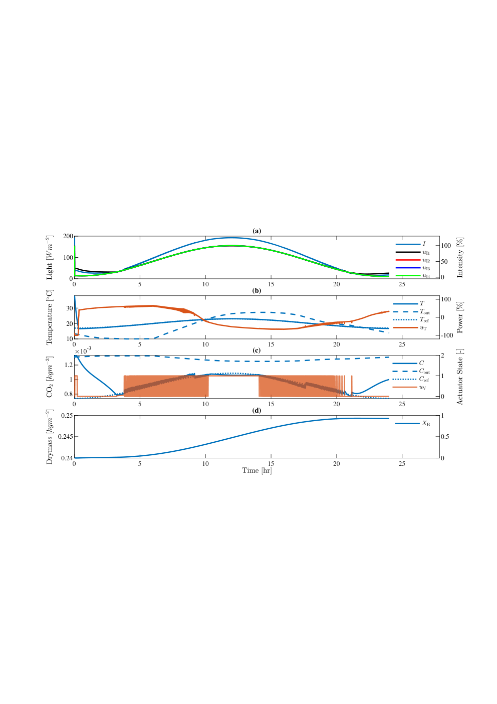
Refer to caption — Figure 2: Simulation results: The model was simulated with the implemented MPC for a duration of 24 hrs. The state trajectories, references, disturbances and the corresponding inputs are visualized. Chattering of certain actuators , e. g., the ventilator, are non-crucial for the production unit used in this work (switching frequency $<0.0333$ Hz).

At first, one can observe constraint satisfaction for all states and inputs according to the specification in the control optimization. The light intensity follows the given reference sinusoid pattern reaching the peak amplitude at noon , i. e., at 12 hr, for all LED channels (see Fig. 2(a)).

Simultaneously, temperature inside the chamber reaches its reference in 0.3 hrs and is able to maintain its reference trajectory for the entire time (see Fig. 2(b)). Jitters in the control signal for the TEC can be noticed at the beginning, around 5-10 hr, and 15-20 hr. These jitters are controller’s response to temperature fluctuation due to the activation of the ventilator (see Fig. 2(c)). It was also observed from simulations with higher $T_{\mathrm{out}}$ temperatures such that the difference $T_{\mathrm{out}}-T^{\mathrm{ref}}>10~^{\circ}$ C, temperature tracking was not achievable. This can be explained by the limitation in heat transfer capacity (cooling) of the actuator(as mentioned previously in Section 2).

CO₂ concentration in the chamber increases at the beginning and at the end of the simulation due to respiration. Since it is not possible to reduce this concentration through ventilation at the mentioned times, the controller increases the light intensity activating photosynthesis and thus CO₂ consumption. At other times, the CO₂ concentration is tracked by frequent switching of the ventilator, providing CO₂ from the outside (see Fig. 2(c)). In the range 0.025-0.2 hr, ventilator is activated to accelerate cooling and thus reach the reference temperature value. It can be noticed that once the light intensity elevates, the CO₂ consumption due to the plant photosynthesis is at maximum requiring constant CO₂ flow. The slew rate used for the ventilator is acceptable for the production unit used in this work. However, for systems with limitation in switching rate, the control problem needs to be modified such that high frequency switching is penalized.

Water levels in the tanks are maintained such that the state constrains (tank capacities) posed on these water levels are not violated. The biomass growth shown in Fig. 2(d) appears to be highest between 7-17 hr when the conditions for growth (temperature and CO₂ concentration) are optimal. Beyond these time points, biomass production rate is minimal.

These simulations depicts certain capability of the tracking control, that could satisfy all state and input constraints according to the specification within the control optimization (21), while also pointing out particular challenges.

5 conclusion

This work reviews the application of a nonlinear predictive controller on a growth chamber for climate tracking control. Specifically, a disturbance affected prediction model of the container-plant-environment interaction was considered, in which particular trajectories have been substituted for the disturbance. Additionally, references for temperature, humidity and CO₂ concentration and light intensity have been specified, representing best growth conditions.

The controller is applied on the nonlinear system, relaxing the binary input constraint to ease the computation. It has been observed that the (heuristic) optimal plant growth environment could be tracked within the limitation of the actuators, while using a short horizon in combination with large sensor and actuator sampling. As for the nonlinearity of the model, further investigations could consider utilizing adaptive control methods in finding efficient control actions that require less computational resources. In a future work, the MPC based controller developed in this work shall be implemented to run on a resource constrained embedded PC.

References

Al-Chalabi (2015) Al-Chalabi, M. (2015). Vertical farming: Skyscraper sustainability? Sustainable Cities and Society, 18, 74 – 77.
Conrad et al. (2017) Conrad, Z., Daniel, S., and Vincent, V. (2017). Vertical farm 2.0: Designing an economically feasible vertical farm - a combined european endeavor for sustainable urban agriculture. Technical report, Association for Vertical Farming.
Ferreau et al. (2007) Ferreau, H.J., Ortner, P., Langthaler, P., del Re, L., and Diehl, M. (2007). Predictive control of a real-world diesel engine using an extended online active set strategy. Annual Rev. Control, 31(2), 293–201.
Gaudreau et al. (1994) Gaudreau, L., Charbonneau, J., VeÌzina, L.P., and Gosselin, A. (1994). Photoperiod and photosynthetic photon flux influence growth and quality of greenhouse-grown lettuce. HortScience HortSci, 29(11), 1285–1289.
Graamans et al. (2018) Graamans, L., Baeza, E., van den Dobbelsteen, A., Tsafaras, I., and Stanghellini, C. (2018). Plant factories versus greenhouses: Comparison of resource use efficiency. Agricultural Systems, 160, 31 – 43.
Gu and Hu (2006) Gu, D. and Hu, H. (2006). Receding horizon tracking control of wheeled mobile robots. IEEE Trans. Control Syst. Tech., 14(4), 743–749.
Henten (1994) Henten, E.v. (1994). Greenhouse climate management : an optimal control approach. Ph.D. thesis, Van Henten, S.l.
Kamel et al. (2017) Kamel, M., Burri, M., and Siegwart, R. (2017). Linear vs nonlinear MPC for trajectory tracking applied to rotary wing micro aerial vehicles. Available at arXiv:1611.09240v2 [cs.RO].
Kim et al. (2002) Kim, H.J., Shim, D.H., and Sastry, S. (2002). Nonlinear model predictive tracking control for rotorcraft-based unmanned aerial vehicles. In Proc. of the American Control Conference.
Kozai (2013) Kozai, T. (2013). Sustainable plant factory: Closed plant production systems with artificial light for high resource use efficiencies and quality produce. Acta Horticulturae, 1004, 27–40.
Murray (1967) Murray, F.W. (1967). On the computation of saturation vapor pressure. Journal of Applied Meteorology, 6(1), 203–204.
Padmanabha and Streif (2019) Padmanabha, M. and Streif, S. (2019). Design and validation of a low cost programmable controlled environment for study and production of plants, mushroom, and insect larvae. Applied Sciences, 9(23).
Rawlings et al. (2012) Rawlings, J.B., Angeli, D., and Bates, C.N. (2012). Fundamentals of economic model predictive control. In Proc. of the 51st IEEE Conference on Decision and Control.
van Straten et al. (2000) van Straten, G., Challa, H., and Buwalda, F. (2000). Towards user accepted optimal control of greenhouse climate. Computers and Electronics in Agriculture, 26(3), 221 – 238.
van Straten et al. (2011) van Straten, G., van Willigenburg, L., van Henten, E., and van Ooteghem, R. (2011). Optimal control of greenhouse cultivation. CRC Press.
Vián et al. (2002) Vián, J., Astrain, D., and Domínguez, M. (2002). Numerical modelling and a design of a thermoelectric dehumidifier. Applied Thermal Engineering, 22(4), 407 – 422.