Robust Design for Intelligent Reflecting Surfaces Assisted MISO Systems

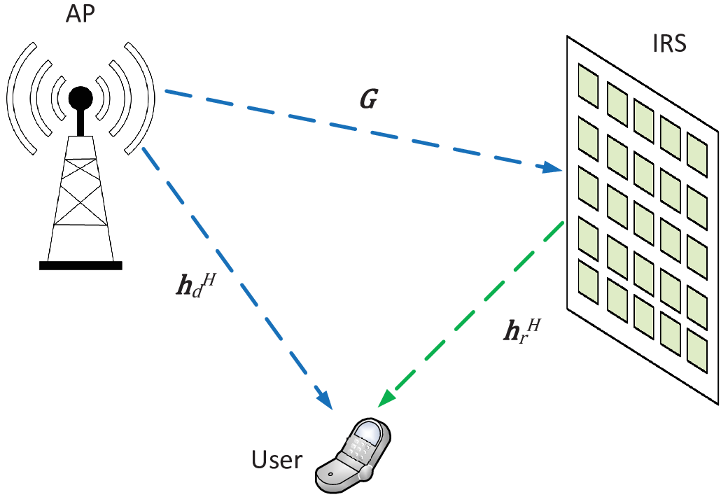
In this section, we consider an IRS-assisted downlink MISO system consisting of one single-antenna user, one AP equipped with $M$ transmit antennas, and one IRS with $N$ passive reflecting elements, as shown in Fig.1. As in [6], the signals reflected by the IRS two or more times are ignored. Thus, the received signal at the user can be given by

where $\textbf{G}\in\mathbb{C}^{N\times M},\textbf{h}_{r}\in\mathbb{C}^{N\times 1},$ $\textbf{h}_{d}\in\mathbb{C}^{M\times 1}$ denote the AP-IRS link, IRS-User link, and AP-User link channels, respectively. Also, $\bm{\Theta}\triangleq{\rm diag}(e^{j\theta_{1}},\cdots,e^{j\theta_{N}})$ is the diagonal reflection matrix of the IRS with $\theta_{n}\in[0,2\pi)$ being the corresponding phase shift. Futhermore, $\textbf{w}\in\mathbb{C}^{M\times 1}$ represents the transmit beamformer at the AP satisfying $||\textbf{w}||^{2}\leq P_{0}$, where $P_{0}$ is the maximum transmit power, while $s$ denotes the zero-mean complex Gaussian symbol with unit power, and $n_{0}$ is the additive white Gaussain noise at the user with zero mean and variance $\sigma_{n}^{2}$.

To detect the transmit symbol, the user applies a one-tap equalizer $c$ and the estimate is given by $\hat{s}=cy$.

As in [12], the CSI errors are assumed to follow the complex Gaussian distribution, namely,

where $\hat{\textbf{G}}$, $\hat{\textbf{h}}_{r}$, and $\hat{\textbf{h}}_{d}$ denote the estimated CSI, and $\Delta\textbf{G}$, $\Delta{\textbf{h}}_{r}$, and $\Delta{\textbf{h}}_{d}$ are the corresponding CSI errors whose entries are i.i.d. zero-mean complex Gaussian with variances of $\sigma_{g}^{2}$, $\sigma_{r}^{2}$, and $\sigma_{d}^{2}$, respectively.

As in [13, 14], the criteria of minimizing the average mean squared error (MSE) is adopted to ensure statistical robustness. Hence, we first write the objective function in the form of MSE averaged over all CSI errors:

where the expectation is taken over the data symbol, additive Gaussian noise, and the CSI errors. Substituting the CSI error model (2) into (3) and using the fact that $\mathbb{E}\{\Delta\textbf{G}^{H}\textbf{H}\Delta\textbf{G}\}=\sigma_{g}^{2}{\rm Tr}\{\textbf{H}\}\textbf{I}_{M}$ for any $\textbf{H}\in\mathbb{C}^{N\times N}$, the MSE expression (3) can be computed as

where A is given by (6) at the bottom of the next page and $\bm{\alpha}=(\hat{\textbf{G}}^{H}\bm{\Theta}^{H}\hat{\textbf{h}}_{r}+\hat{\textbf{h}}_{d})$. Subject to the power constraint at the AP and the unit-modulus constraint at the IRS, the joint design of the transceiver and IRS phase shifts can be formulated as

Note that the objective function (4) is non-convex with respect to (w.r.t.) w, $c,$ and $\bm{\Theta}$, which makes the optimization problem (P1) very difficult to solve. In the following, we propose an AO method to solve it.

First we update the beamfoming vector w and one-tap equalizer $c$ for a given phase shift matrix $\bm{\Theta}$. Specifically, given an arbitrary fixed $\bm{\Theta}$, the original problem (P1) can be reformulated as follows:

It can be observed that the objective function is non-convex w.r.t. w and $c$, hence, we optimize w and $c$ alternatingly. Given w, the optimal equalizer $c$ for the problem (7) is known to be the classical Wiener filter [15]:

Then, for a fixed $c$, the optimal beamforming vector w derived by using the Lagrangian method. The Lagrangian function for (7) is given by

where $e(\textbf{w})$ is given in (7) and $\lambda$ is the Lagrange multiplier associated with w. Taking the derivative of (9) w.r.t. beamformer $\textbf{w}^{*}$, we can find the optimal solutions for (7) with the Karush–Kuhn–Tucker conditions [16]:

It is obvious that (10) is sufficient and necessary for the optimal. As shown in (10), the optimal w depends on the Lagrange multiplier $\lambda$, thus $\lambda$ should be calculated first before computing the beamformer w. According to (10c), either $\lambda=0$ or $||\textbf{w}||^{2}=P_{0}$ must hold. Hence, if $\lambda=0$ and $||\textbf{w}||^{2}-P_{0}\leq 0$ is satisfied, then $\lambda=0$. In contrast, if $\lambda=0$, but $||\textbf{w}||^{2}-P_{0}\leq 0$ is not satisfied, then we have to solve the equation $||\textbf{w}||^{2}=P_{0}$, which can be done numerically using the bisection search method. After $\lambda$ is obtained, we then calculate the beamformer w according to (10).

Now we optimize the phase shift matrix $\bm{\Theta}$ with fixed w and $c$. For simplicity, we omit the constant terms in (4) and rewrite the objective function of (P1) as

Let $\textbf{v}\triangleq[v_{1},\cdots,v_{N}]^{H}$ where $v_{i}=e^{j\theta_{i}}$ for all $i=1,\cdots,N$, $\bm{\Phi}={\rm diag}(\hat{\textbf{h}}_{r}^{H})\hat{\textbf{G}}\textbf{w}c$ and ${d}=\hat{\textbf{h}}_{d}^{H}\textbf{w}c$, then we have $\hat{\textbf{h}}_{r}^{H}\bm{\Theta}_{i+1}\hat{\textbf{G}}\textbf{w}c=\textbf{v}^{H}\bm{\Phi}$. As such, (11) can be rewritten as

Hence, the corresponding optimization problem can be recast as nonconvex quadratically constrained quadratic programs (QCQPs)

Due to the unit modulus constraint, the above problem is non-convex, and belongs to the class of NP-hard problems. The conventional approach is to reformulate the above problem as semidefinite programming problem via matrix-lifting [17]. However, as the number of reflecting elements grows large, the implementation of the matrix-lifting procedure is challenging.

Therefore, we propose a MM based method to solve (13). The MM algorithm is an iterative technique to find an absolute minimizer. Instead of minimizing $f(\textbf{v})$, this method minimizes a majorization function of $f(\textbf{v})$ at each iteration point. The $k$th majorizer for the objective function should satisfy the following two conditions:

where $\textbf{v}_{k-1}$ is the value of v at the $(k-1)$th iteration. Indeed, the function $g(\textbf{v},\textbf{v}_{k-1})$ is an upper bound of the function $f(\textbf{v})$ and the equality is achieved at point $\textbf{v}_{k-1}$. To ensure a monotonically decreasing sequence of the function values, each iterative value $\textbf{v}_{k}$ follows the update rule $\textbf{v}_{k}=\rm{argmin}\ g(\textbf{v},\textbf{v}_{k-1})$. So we have:

Hence, the key in MM algorithm is to determine the majorizer $g(\textbf{v},\textbf{v}_{k-1})$ such that the majorized problem is easy to solve. To apply the MM technique, we first rewrite problem (13) as

where $\textbf{Q}=\bm{\Phi}\bm{\Phi}^{H}$ is a positive semidefinite matrix and $\textbf{q}=\bm{\Phi}(1-d^{*})$. Invoking the Claim 1 of [19], the function $\textbf{v}^{H}\textbf{Q}\textbf{v}$ can be majorized by $\textbf{v}^{H}\textbf{H}\textbf{v}+2\mathcal{R}(\textbf{v}^{H}(\textbf{Q}-\textbf{H})\textbf{v}_{0})+\textbf{v}_{0}^{H}(\textbf{H}-\textbf{Q})\textbf{v}_{0}$ at every $\textbf{v}_{0}\in\mathbb{C}^{N}$, where H is a fixed matrix such that $\textbf{H}\succeq\textbf{Q}$. Thus, the majorized problem of (16) can be expressed as

Let $\textbf{H}=\lambda_{max}(\textbf{Q})\textbf{I}$ where $\lambda_{max}(\textbf{Q})$ is the largest eigenvalue of matrix Q, so that the first term of (17) is a constant. By discarding constant terms w.r.t. v, the new majorization problem at the ($k+1$)th iteration is

where u = ${(\textbf{Q}-\lambda_{max}(\textbf{Q})\textbf{I})}\textbf{v}_{k}-\textbf{q}$ is a constant w.r.t. the variable v since the vector $\textbf{v}_{k}$ is known beforehand by generating at iteration $k$. Thus, the optimal solution to problem (18) is given by

at the ($k+1$)th iteration. Since the monotonicity of the MM algorithm ensures that $f(\textbf{v}_{i})\leq f(\textbf{v}_{j})$ for all $i>j$, we can repeat the above steps to find a stationary point and the phase shifts $\bm{\Theta}$ can be easily recovered from $\textbf{v}^{*}$.

In summary, the overall AO algorithm yields a simple closed-form solution at every iteration, which is given in Algorithm 1. As shown, the optimal solutions {$\textbf{w}^{t},c^{t}$} and locally optimal solution $\bm{\Theta}^{t}$ are obtained alternatingly, with superscript $t$ denoting the $t$th iteration.

The proposed AO algorithm can be shown to converge as follows. Recall the objective function of problem (P1) and it follows that

The first inequality holds due to the non-increasing property of the general MM scheme. The last two inequalities come from (10) and (8), i.e., $\textbf{w}^{t+1}$ and $c^{t+1}$ corresponds to the minimizer of $e(\textbf{w},c^{t+1},\bm{\Theta}^{t})$ and $e(\textbf{w}^{t},c,\bm{\Theta}^{t})$, respectively.

Furthermore, we briefly discuss the computational complexity of the proposed AO algorithm. In each iteration, the algorithm yields simple closed-form solutions and only requires basic matrix operations. Firstly, as for updating the transcievr $\textbf{w},c$, the complexity to calculate A is on the order of $\mathcal{O}(M^{2}N)$. Also, the complexity to find the optimal $\lambda$ is about $\mathcal{O}(log(m)M^{3})$, where $m$ denotes the interval length of the bisection search. Secondly, as for updating the IRS phase shifts, the algorithm requires the computational complexity of $\mathcal{O}(n(NM+N^{2}))$ for the matrix multiplications, where $n$ represents the number of MM algorithm iterations. The overall computational complexity of each iteration is given by $\mathcal{O}(M^{2}N+log(m)M^{3}+n(NM+N^{2}))$.

References

- [1] W. Tang, et al, “MIMO transmission through reconfigurable intelligent surface: System design, analysis, and implementation,” arXiv: abs/1912.09955, Dec. 2019.
- [2] Y. Han, et al, “Large intelligent surface-assisted wireless communication exploiting statistical CSI,” IEEE Trans. Veh. Tech., vol. 68, no. 8, pp. 8238-8242, Aug. 2019.
- [3] X. Hu, C. Zhong, Y. Zhu, X. Chen, and Z. Zhang, “Programmable metasurface based multicast systems: Design and analysis,” accepted to appear in IEEE J. Selected Areas in Commun., 2020.
- [4] J. Gao, C. Zhong, X. Chen, H. Lin, and Z. Zhang, “Unsupervised learning for passive beamforming,” IEEE Commun. Lett., vol. 24, no. 5, pp. 1052-1056, May 2020.
- [5] Y. Zhang, C. Zhong, Z. Zhang, and W. Lu, “Sum rate optimization for two way communications with intelligent reflecting surface,” IEEE Commun. Lett., vol. 24, no. 5, pp. 1090-1094, May 2020.
- [6] Q. Wu and R. Zhang, “Intelligent reflecting surface enhanced wireless network: Joint active and passive beamforming design,” in Proc. IEEE GLOBECOM, Abu Dhabi, United Arab Emirates, pp. 1-6, Dec. 2018.
- [7] Q. Wu and R. Zhang, “Beamforming optimization for intelligent reflecting surface with discrete phase shifts,” in Proc. IEEE ICASSP, Brighton, United Kingdom, pp. 7830-7833, May 2019.
- [8] X. Yu, D. Xu, and R. Schober, “Enabling secure wireless communications via intelligent reflecting surfaces,” arXiv: abs/1904.09573, Apr. 2019.
- [9] X. Guan, Q. Wu and R. Zhang, “Intelligent reflecting surface assisted secrecy communication: Is artificial noise helpful or not?,” accepted to appear in IEEE Wireless Commun. Lett., 2020.
- [10] G. Araujo and A. Almeida, “Parafac-based channel estimation for intelligent reflective surface assisted MIMO system,” arXiv: abs/2001.06554, Jan. 2020.
- [11] D. R. Hunter and K. Lange, “A tutorial on MM algorithms,” The American Statistician, vol. 58, no. 1, pp. 30-37, Feb. 2004.
- [12] G. Zheng, S. Ma, K.-K. Wong, and T.-S. Ng, “Robust beamforming in cognitive radio,” IEEE Trans. Wireless Commun., vol. 9, no. 2, pp. 570-576, Feb. 2010.
- [13] C. Xing, S. Ma, and Y.-C. Wu, “Robust joint design of linear relay precoder and destination equalizer for dual-hop amplify-and-forward MIMO relay systems,” IEEE Trans. Sig. Process., vol. 58, no. 4, pp. 2273–2283, Apr. 2010.
- [14] H. Shen, W. Xu, and C. Zhao, “Robust transceiver for AF MIMO relaying with direct link: A globally optimal solution,” IEEE Sig. Process. Lett., vol. 21, no. 8, pp. 947–951, Aug. 2014.
- [15] D. G. Manolakis, V. K. Ingle, and S. M. Kogon, Statistical and Adaptive Signal Processing: Spectral Estimation, Signal Modeling, Adaptive Filtering and Array Processing. New York: The McGraw-Hill Companies, Inc., 2000
- [16] S. Boyd and L. Vandenberghe, Convex Optimization. Cambridge, U.K.: Cambridge University Press, 2004.
- [17] S. Zhang and Y. Huang, “Complex quadratic optimization and semidefinite programming,” SIAM Journal on Optimization, vol. 16, no. 3, pp. 871–890, July 2006.
- [18] S. Gong, C. Xing, and V. Lau, “Majorization-minimization aided hybrid transceivers for MIMO interference channels,” arXiv: abs/1911.05906, Nov. 2019.
- [19] T. Qiu, P. Babu, and D. P. Palomar, “Prime: Phase retrieval via majorization-minimization,” IEEE Trans. Sig. Process., vol. 64, no. 19, pp. 5174-5186, Oct. 2016.