Getting a CLUE: A Method for
Explaining Uncertainty Estimates
Abstract
Both uncertainty estimation and interpretability are important factors for trustworthy machine learning systems. However, there is little work at the intersection of these two areas. We address this gap by proposing a novel method for interpreting uncertainty estimates from differentiable probabilistic models, like Bayesian Neural Networks (BNNs). Our method, Counterfactual Latent Uncertainty Explanations (CLUE), indicates how to change an input, while keeping it on the data manifold, such that a BNN becomes more confident about the input’s prediction. We validate CLUE through 1) a novel framework for evaluating counterfactual explanations of uncertainty, 2) a series of ablation experiments, and 3) a user study. Our experiments show that CLUE outperforms baselines and enables practitioners to better understand which input patterns are responsible for predictive uncertainty.
1 Introduction
There is growing interest in probabilistic machine learning models, which aim to provide reliable estimates of uncertainty about their predictions (MacKay 1992). These estimates are helpful in high-stakes applications such as predicting loan defaults or recidivism, or in work towards autonomous vehicles. Well-calibrated uncertainty can be as important as making accurate predictions, leading to increased robustness of automated decision-making systems and helping prevent systems from behaving erratically for out-of-distribution (OOD) test points. In practice, predictive uncertainty conveys skepticism about a model’s output. However, its utility need not stop there: we posit predictive uncertainty could be rendered more useful and actionable if it were expressed in terms of model inputs, answering the question: “Which input patterns lead my prediction to be uncertain?”
Understanding which input features are responsible for predictive uncertainty can help practitioners learn in which regions the training data is sparse. For example, when training a loan default predictor, a data scientist (i.e., practitioner) can identify sub-groups (by age, gender, race, etc.) under-represented in the training data. Collecting more data from these groups, and thus further constraining their model’s parameters, could lead to accurate predictions for a broader range of clients. In a clinical scenario, a doctor (i.e., domain expert) can use an automated decision-making system to assess whether a patient should receive a treatment. In the case of high uncertainty, the system would suggest that the doctor should not rely on its output. If uncertainty were explained in terms of which features the model finds anomalous, the doctor could appropriately direct their attention.
While explaining predictions from deep models has become a burgeoning field (Montavon et al. 2018; Bhatt et al. 2020b), there has been relatively little research on explaining what leads to neural networks’ predictive uncertainty. In this work, we introduce Counterfactual Latent Uncertainty Explanations (CLUE), to our knowledge, the first approach to shed light on the subset of input space features that are responsible for uncertainty in probabilistic models. Specifically, we focus on explaining Bayesian Neural Networks (BNNs). We refer to the explanations given by our method as CLUEs. CLUEs try to answer the question: “What is the smallest change that could be made to an input, while keeping it in distribution, so that our model becomes certain in its decision for said input?” CLUEs can be generated for tabular and image data on both classification and regression tasks.

An application of CLUE is to improve transparency in the real-world deployment of a probabilistic model, such as a BNN, by complementing existing approaches to model interpretability (Ribeiro et al. 2016; Sundararajan et al. 2017; Chang et al. 2019). When the BNN is confident in its prediction, practitioners can generate an explanation via earlier feature importance techniques. When the BNN is uncertain, its prediction may well be wrong. This potentially wrong prediction could be the result of factors not related to the actual patterns present in the input data, e.g. parameter initialization, randomness in mini-batch construction, etc. An explanation of an uncertain prediction will be disproportionately affected by these factors. Indeed, recent work on feature attribution touches on the unreliability of saliency maps when test points are OOD (Adebayo et al. 2020). Therefore, when the BNN is uncertain, it makes sense to provide an explanation of why the BNN is uncertain (i.e., CLUE) instead of an explanation of the BNN’s prediction. This is illustrated in Figure 1. Our code is at: github.com/cambridge-mlg/CLUE. We highlight the following contributions:
- •
We introduce CLUE, an approach that finds counterfactual explanations of uncertainty in input space, by searching in the latent space of a deep generative model (DGM). We put forth an algorithm for generating CLUEs and show how CLUEs are best displayed.
- •
We propose a computationally grounded approach for evaluating counterfactual explanations of uncertainty. It leverages a separate conditional DGM as a synthetic data generator, allowing us to quantify how well explanations reflect the true generative process of the data.
- •
We evaluate CLUE quantitatively through comparison to baseline approaches under the above framework and through ablative analysis. We also perform a user study, showing that CLUEs allow practitioners to predict on which new inputs a BNN will be uncertain.
2 Preliminaries
2.1 Uncertainty in BNNs
Given a dataset , a prior on our model’s weights , and a likelihood function , the posterior distribution over the predictor’s parameters encodes our uncertainty about what value should take. Through marginalization, this parameter uncertainty is translated into predictive uncertainty, yielding reliable error bounds and preventing overfitting:
| (1) |
For BNNs, both the posterior over parameters and predictive distribution Equation 1 are intractable. Fortunately, there is a rich literature concerning approximations to these objects (MacKay 1992; Hernández-Lobato & Adams 2015; Gal 2016). In this work, we use scale-adapted Stochastic Gradient Hamiltonian Monte Carlo (SG-HMC) (Springenberg et al. 2016). For regression, we use heteroscedastic Gaussian likelihood functions, quantifying uncertainty using their standard deviation, . For classification, we take the entropy of categorical distributions as uncertainty. Details are given in Appendix B. Hereafter, we use to refer to any uncertainty metric, be it or .
Predictive uncertainty can be separated into two components, as shown in Figure 2. Each conveys different information to practitioners (Depeweg 2019). Irreducible or aleatoric uncertainty is caused by inherent noise in the generative process of the data, usually manifesting as class overlap. Model or epistemic uncertainty represents our lack of knowledge about . Stemming from a model being under-specified by the data, epistemic uncertainty arises when we query points off the training manifold. Capturing model uncertainty is the main advantage of BNNs over regular NNs. It enables the former to be used for uncertainty aware tasks, such as OOD detection (Daxberger & Hernández-Lobato 2019), continual learning (Nguyen et al. 2018), active learning (Depeweg et al. 2018), and Bayesian optimization (Springenberg et al. 2016).

2.2 Uncertainty Sensitivity Analysis
To the best of our knowledge, the only existing method for interpreting uncertainty estimates is Uncertainty Sensitivity Analysis (Depeweg et al. 2017). This method quantifies the global importance of an input dimension to a chosen metric of uncertainty using a sum of linear approximations centered at each test point:
| (2) |
As discussed by Rudin 2019, linear explanations of non-linear models, such as BNNs, can be misleading. Even generalized linear models, which are often considered to be “inherently interpretable,” like logistic regression, produce non-linear uncertainty estimates in input space. This can be seen in Figure 2. Furthermore, high-dimensional input spaces limit the actionability of these explanations, as will likely not point in the direction of the data manifold. In Figure 3 and Appendix D, we show how this can result in sensitivity analysis generating meaningless explanations.
Our method, CLUE, leverages the latent space of a DGM to avoid working with high-dimensional input spaces and to ensure explanations are in-distribution. CLUE does not rely on crude linear approximations. The counterfactual nature of CLUE guarantees explanations have tangible meaning.

2.3 Counterfactual Explanations
The term “counterfactual” captures notions of what would have happened if something had been different. Two meanings have been used by ML subcommunities. 1) Those in causal inference make causal assumptions about interdependencies among variables and use these assumptions to incorporate consequential adjustments when particular variables are set to new values (Kusner et al. 2017; Pearl 2019). 2) In contrast, the interpretability community recently used “counterfactual explanations” to explore how input variables must be modified to change a model’s output without making explicit causal assumptions (Wachter et al. 2018). As such, counterfactual explanations can be seen as a case of contrastive explanations (Dhurandhar et al. 2018; Byrne 2019). In this work, we use “counterfactual” in a sense similar to 2): we seek to make small changes to an input in order to reduce the uncertainty assigned to it by our model, without explicit causal assumptions.
Multiple counterfactual explanations can exist for any given input, as the functions we are interested in explaining are often non-injective (Russell 2019). We are concerned with counterfactual input configurations that are close to the original input according to some pairwise distance metric . Given a desired outcome different from the original one produced by predictor , counterfactual explanations are usually generated by solving an optimization problem that resembles:
| (3) |
Naively optimizing Equation 3 in high-dimensional input spaces may result in the creation of adversarial inputs which are not actionable (Goodfellow et al. 2015). Telling a person that they would have been approved for a loan had their age been is of very little use. To right this, recent works define linear constraints on explanations (Ustun et al. 2019; Sharma et al. 2020). An alternative more amenable to high dimensional data is to leverage DGMs (which we dub auxiliary DGMs) to ensure explanations are in-distribution (Dhurandhar et al. 2018; Joshi et al. 2018; Chang et al. 2019; Booth et al. 2020; Tripp et al. 2020). CLUE avoids the above issues by searching for counterfactuals in the lower-dimensional latent space of an auxiliary DGM. This choice is well suited for uncertainty, as the DGM constrains CLUE’s search space to the data manifold. When faced with an OOD input, CLUE returns the nearest in-distribution analog, as shown in Figure 3.
3 Proposed Method
Without loss of generality, we use to refer to any differentiable estimate of uncertainty ( or ). We introduce an auxiliary latent variable DGM: . In the rest of this paper, we will use the decoder from a variational autoencoder (VAE). Its encoder is denoted as . We write these models’ predictive means as and respectively.
CLUE aims to find points in latent space which generate inputs similar to an original observation but are assigned low uncertainty. This is achieved by minimizing Equation 4. CLUEs are then decoded as Equation 5.
| (4) | |||
| (5) |
The pairwise distance metric takes the form such that we can enforce similarity between uncertain points and CLUEs in both input and prediction space. The hyperparameters control the trade-off between producing low uncertainty CLUEs and CLUEs which are close to the original inputs. In this work, we take to encourage sparse explanations. For regression, is mean squared error. For classification, we use cross-entropy. Note that the best choice for will be task-specific.

The CLUE algorithm and a diagram of our procedure are provided in Algorithm 1 and Figure 4, respectively. The hyperparameter is selected by cross validation for each dataset such that both terms in Equation 4 are of similar magnitude. We set to for our main experiments, but explore different values in Section H.1. We minimize Equation 4 with Adam by differentiating through both our BNN and VAE decoder. To facilitate optimization, the initial value of is chosen to be . Optimization runs for a minimum of three iterations and a maximum of iterations, with a learning rate of . If the decrease in is smaller than for three consecutive iterations, we apply early stopping. CLUE can be applied to batches of inputs simultaneously, allowing us to leverage GPU-accelerated matrix computation. Our implementation is detailed in full in Appendix B.
As noted by Wachter et al. 2018, individual counterfactuals may not shed light on all important features. Fortunately, we can exploit the non-convexity of CLUE’s objective to address this. We initialize CLUE with , where , and perform Algorithm 1 multiple times to obtain different CLUEs. We find to give a good trade-off between optimization speed and CLUE diversity. Appendix C shows examples of different CLUEs obtained for the same inputs.


We want to ensure noise from auxiliary DGM reconstruction does not affect CLUE visualization. For tabular data, we use the change in percentile of each input feature with respect to the training distribution as a measure of importance. We only highlight continuous variables for which CLUEs are separated by percentile points or more from their original inputs. All changes to discrete variables are highlighted. For images, we report changes in pixel values by applying a sign-preserving quadratic function to the difference between CLUEs and original samples: with . This is showcased in Figure 5 and in Appendix G. It is common for approaches to generating saliency maps to employ constraints that encourage the contiguity of highlighted pixels (Chang et al. 2019; Dabkowski & Gal 2017). We do not employ such constraints, but we note they might prove useful when applying CLUE to natural images.
4 A Framework for Evaluating Counterfactual Explanations of Uncertainty Computationally
Evaluating explanations quantitatively (without resorting to expensive user studies) is a difficult but important task (Doshi-Velez & Kim 2017; Weller 2019). We put forth a computational framework to evaluate counterfactual explanations of uncertainty. In the spirit of Bhatt et al. 2020a, we desire counterfactuals that are 1) informative: they should highlight features which affect our BNN’s uncertainty, and 2) relevant: counterfactuals should lie close to the original inputs and represent plausible parameter settings, lying close to the data manifold. Recall, from Figure 3, that inputs for which our BNN is certain can be constructed by applying adversarial perturbations to uncertain ones. Alas, evaluating these criteria requires access to the generative process of the data.
To evaluate the above requirements, we introduce an additional DGM that will act as a “ground truth” data generating process (g.t. DGM). Specifically, we use a variational autoencoder with arbitrary conditioning (Ivanov et al. 2019) (g.t. VAEAC).

It jointly models inputs and targets . Measuring counterfactuals’ log density under this model allows us to evaluate if they are in-distribution. The g.t. VAEAC also allows us to query the conditional distribution over targets given inputs, . From this distribution, we can compute an input’s true uncertainty , as given by the generative process of the data. This allows us to evaluate if counterfactuals address the true sources of uncertainty in the data, as opposed to exploiting adversarial vulnerabilities in the BNN. The evaluation procedure, shown in Figure 6, is as follows:
- 1.
Train a g.t. VAEAC on a real dataset to obtain as well as conditionals .
- 2.
Sample artificial data . Use them to train a BNN and an auxiliary DGM.
- 3.
Sample more artificial data. Generate counterfactual explanations for uncertain samples.
- 4.
Use the g.t. VAEAC to obtain the conditional distribution over targets given counterfactual inputs and . Evaluate if counterfactuals are on-manifold through .
Given an uncertain artificially generated test point and its corresponding counterfactual explanation , we quantify informativeness as the amount of uncertainty that has been explained away. The variance (or entropy) of reflects the ground truth aleatoric uncertainty associated with . Hence, for aleatoric uncertainty, we quantify informativeness as . Epistemic uncertainty only depends on our BNN. It cannot be directly computed from . However, its reduction can be measured implicitly through the reduction in the BNN’s prediction error with respect to the labels outputted by the g.t. VAEAC: . Here . Approaches that exploit adversarial weaknesses in the BNN will not transfer to the g.t. VAEAC, failing to reduce uncertainty or error. We assess the relevance of counterfactuals through their likelihood under the g.t. VAEAC and through their distance to the original inputs . We refer to Appendix I for a detailed discussion on g.t. VAEACs and their use for comparing counterfactual generations.
5 Experiments
We validate CLUE on LSAT academic performance regression (Wightman et al. 1998), UCI Wine quality regression, UCI Credit classification (Dua & Graff 2017), a feature variant of COMPAS recidivism classification (Angwin et al.), and MNIST image classification (LeCun & Cortes 2010). For each, we select roughly the most uncertain test points as those for which we reject our BNNs’ decisions. We only generate CLUEs for “rejected” points. Rejection thresholds, architectures, and hyperparameters are in Appendix B. Experiments with non-Bayesian NNs are in Section H.1.
As a baseline, we introduce a localized version of Uncertainty Sensitivity Analysis (Depeweg et al. 2017). It produces counterfactuals by taking a single step, of size , in the direction of the gradient of an input’s uncertainty estimates . Averaging across a test set, we recover Equation 2. As a second baseline, we adapt FIDO (Chang et al. 2019), a counterfactual feature importance method, to minimize uncertainty. We dub this approach U-FIDO. This method places a binary mask over the set of input variables . The mask is modeled by a product of Bernoulli random variables: . The set of masked inputs is substituted by its expectation under an auxiliary conditional generative model . We use a VAEAC. U-FIDO finds the masking parameters which minimize Equation 6:
| (6) | ||||
| (7) |
Counterfactuals are generated by Equation 7, where is the Hadamard product. We compare CLUE to feature importance methods (Ribeiro et al. 2016; Lundberg & Lee 2017) in Appendix F.
5.1 Computational Evaluation
We compare CLUE, Localized Sensitivity, and U-FIDO using the evaluation framework put forth in Section 4. We would like counterfactuals to explain away as much uncertainty as possible while staying as close to the original inputs as possible. We manage this informativeness (large ) to relevance (small ) trade-off with the hyperparameters , , and for Local Sensitivity, CLUE, and U-FIDO, respectively. We perform a logarithmic grid search over hyperparameters and plot Pareto-like curves. Our two metrics of interest take minimum values of but their maximum is dataset and method dependent. For Sensitivity, grows linearly with . For CLUE and U-FIDO, these metrics saturate for large and small values of (or ). As a result, the values obtained by these methods do not overlap. As shown in Figure 7, CLUE is able to explain away more uncertainty () than U-FIDO, and U-FIDO always obtains smaller values of than CLUE.
| Method | LSAT (4) | COMPAS (7) | Wine (11) | Credit (23) | MNIST (784) | |||||
|---|---|---|---|---|---|---|---|---|---|---|
| e | a | e | a | e | a | e | a | e | a | |
| Sensitivity | 0.70 | 0.67 | 0.71 | 0.13 | 0.69 | 0.03 | 0.63 | 0.50 | 0.66 | 0.68 |
| CLUE | 0.52 | 0.64 | 0.71 | 0.18 | 0.01 | 0.14 | 0.52 | 0.29 | 0.26 | 0.27 |
| U-FIDO | 0.36 | 0.51 | 0.71 | 0.31 | 0.22 | 0.02 | 0.45 | 0.63 | 0.38 | 0.50 |
To construct a single performance metric, we scale all measurements by the maximum values obtained between U-FIDO or CLUE, e.g. , linearly mapping them to . We then negate , making its optimum value . We consider each method’s best performing hyperparameter configuration, as determined by its curve’s point nearest the origin, or knee-point. The euclidean distance from each method’s knee-point to the origin acts as a metric of relative performance. The best value is and the worst is . Knee-point distances, computed across three runs, are shown for both uncertainty types in Table 1.
Local Sensitivity performs poorly on all datasets except COMPAS. We attribute this to the implicit low dimensionality of COMPAS: only two features are necessary to accurately predict targets (Dressel & Farid 2018). U-FIDO’s masking mechanism allows for counterfactuals that leave features unchanged. It performs well in low dimensional problems but suffers from variance as dimensionality grows. We conjecture that optimization in latent (instead of input) space makes CLUE robust to data complexity.
We perform an analogous experiment where relevance is quantified as proximity to the data manifold: . Here, refers to the log-likelihood of the artificial data for which counterfactuals are generated. Results are in Table 2, where CLUE performs best in tasks. Generating counterfactuals with a VAE ensures that CLUEs are relevant. In Section H.2, we perform an analogous informativeness vs relevance experiment on real data. We obtain similar results to our computational evaluation framework, validating its reliability.
| Method | LSAT (4) | COMPAS (7) | Wine (11) | Credit (23) | MNIST (784) | |||||
|---|---|---|---|---|---|---|---|---|---|---|
| e | a | e | a | e | a | e | a | e | a | |
| Sensitivity | 0.697 | 0.672 | 0.707 | 0.122 | 0.691 | 0.001 | 0.623 | 0.454 | 0.682 | 0.698 |
| CLUE | 0.419 | 0.070 | 0.707 | 0.044 | 0 | 0.128 | 0 | 0.009 | 0.273 | 0.146 |
| U-FIDO | 0 | 0 | 0.707 | 0.303 | 0.224 | 0 | 0.233 | 0.628 | 0.450 | 0.516 |
5.2 User Study
Human-based evaluation is a key step in validating the utility of tools for ML explainability (Hoffman et al. 2018). We want to assess the extent to which CLUEs help machine learning practitioners identify sources of uncertainty in ML models compared to using simple linear approximations (Local Sensitivity) or human intuition. To do this, we propose a forward-simulation task (Doshi-Velez & Kim 2017), focusing on an appropriate local test to evaluate CLUEs. We show practitioners one datapoint below our “rejection” threshold and one datapoint above. The former is labeled as “certain” and the latter as “uncertain”; we refer to these as context points. The certain context point serves as a local counterfactual explanation for the uncertain context point. Using both context points for reference, practitioners are asked to predict whether a new test point will be above or below our threshold (i.e., will our BNN’s uncertainty be high or low for the new point). Our survey compares the utility of the certain context points generated by CLUE relative to those from baselines.


In our survey, we compare four different methods, varying how we select certain context points. We either 1) select a certain point at random from the test set as a control, generate a counterfactual certain point with 2) Local Sensitivity or with 3) CLUE, or 4) display a human selected certain point (Human CLUE). To generate a Human CLUE, we ask participants (who will not take the main survey) to pair uncertain context points with similar certain points. We select the points used in our main survey with a pilot procedure similar to Grgic-Hlaca et al. 2018. This procedure, shown in Figure 8, prevents us from injecting biases into point selection and ensures context points are relevant to test points. In our procedure, a participant is shown a pool of randomly selected certain and uncertain points. We ask this participant to select points from this pool: these will be test points. We then ask the participant to map each selected test point to a similar uncertain point without replacement. In this way, we obtain uncertain context points that are relevant to test points.
We use the LSAT and COMPAS datasets in our user study. Ten different participants take each variant of the main survey: our participants are ML graduate students, who serve as proxies for practitioners in industry. The main survey consists of questions, per dataset. An example question is shown in Figure 9. The average participant accuracy by variant is: CLUE (), Human CLUE (), Random (), and Local Sensitivity (). We measure the statistical significance of CLUE’s superiority with unpaired Wilcoxon signed-rank tests (Demšar 2006) of CLUE vs each baseline. We obtain the following p-values: Human-CLUE (), Random (), and Sensitivity ().11 1 Our between-group experimental design could potentially result in dependent observations, which violates the tests’ assumptions. However, the p-values obtained are extremely low, providing confidence in rejecting the null hypothesis of equal performance among approaches. Additional analysis is included in Section H.3.
We find that linear explanations (Local Sensitivity) of a non-linear function (BNN) mislead practitioners and perform worse than random. While Human CLUE explanations are real datapoints, CLUE generates explanations from a VAE. We conjecture that CLUE’s increased flexibility produces relevant explanations in a broader range of cases. In our tabular data user study, we only show one pair of context points per test point. We find that otherwise the survey is difficult for practitioners to follow, due to non-expertise in college admissions or criminal justice. Using MNIST, we run a smaller scale study, wherein we show participants larger sets of context points. Results are in Section J.2.
5.3 Analysis of CLUE’s Auxiliary Deep Generative Model
We study CLUE’s reliance on its auxiliary DGM. Further ablative analysis is found in Appendix H.
Initialization Strategy: We compare Algorithm 1’s encoder-based initialization with . As shown in Figure 10, for high dimensional datasets, like MNIST, initializing with the encoder’s mean leads to CLUEs that require smaller changes in input space to explain away similar amounts of uncertainty (i.e., more relevant). In Section H.1, similar behavior is observed for Credit, our second highest dimensional dataset. On other datasets, both approaches yield indistinguishable results. CLUEs could plausibly be generated with differentiable DGMs that lack an encoding mechanism, such as GANs. However, an appropriate initialization strategy should be employed.
Capacity of CLUE’s DGM: Figure 10 shows how auto-encoding uncertain MNIST samples with low-capacity VAEs significantly reduces these points’ predictive entropy. CLUEs generated with these VAEs highlight features that the VAEs are unable to reproduce but are not reflective of our BNN’s uncertainty. This results in large values of ; although the counterfactual examples are indeed more certain than the original samples, they contain unnecessary changes. As our auxiliary DGMs’ capacity increases, the amount of uncertainty preserved when auto-encoding inputs increases as well. decreases while the predictive entropy of our CLUEs stays the same. More expressive DGMs allow for generating sparser, more relevant, CLUEs. Fortunately, even in scenarios where our predictor’s training dataset is limited, we can train powerful DGMs by leveraging unlabeled data.

6 Conclusion
With the widespread adoption of data-driven decision making has come a need for the development of ML tools that can be trusted by their users. This has spawned a subfield of ML dedicated to interpreting deep learning systems’ predictions. A transparent deep learning method should also inform stakeholders when it does not know the correct prediction (Bhatt et al. 2021). In turn, this creates a need for being able to interpret why deep learning methods are uncertain.
We address this issue with Counterfactual Latent Uncertainty Explanations (CLUE), a method that reveals which input features can be changed to reduce the uncertainty of a probabilistic model, like a BNN. We then turn to assessing the utility, to stakeholders, of counterfactual explanations of predictive uncertainty. We put forth a framework for computational evaluation of these types of explanations. Quantitatively, CLUE outperforms simple baselines. Finally, we perform a user study. It finds that users are better able to predict their models’ behavior after being exposed to CLUEs.
Acknowledgements
JA acknowledges support from Microsoft Research through its PhD Scholarship Program. UB acknowledges support from DeepMind and the Leverhulme Trust via the Leverhulme Centre for the Future of Intelligence (CFI) and from the Mozilla Foundation. AW acknowledges support from a Turing AI Fellowship under grant EP/V025379/1, The Alan Turing Institute under EPSRC grant EP/N510129/1 & TU/B/000074, and the Leverhulme Trust via CFI.
References
- Adebayo et al. (2020) Julius Adebayo, Michael Muelly, Ilaria Liccardi, and Been Kim. Debugging tests for model explanations. Advances in Neural Information Processing Systems, 33, 2020.
- (2) Julia Angwin, Jeff Larson, Surya Mattu, and Lauren Kirchner. Machine bias. there’s software used across the country to predict future criminals. and it’s biased against blacks. URL https://www.propublica.org/article/machine-bias-risk-assessments-in-criminal-sentencing.
- Antoran & Miguel (2019) J. Antoran and A. Miguel. Disentangling and learning robust representations with natural clustering. In 2019 18th IEEE International Conference On Machine Learning And Applications (ICMLA), pp. 694–699, 2019.
- Bengio (2013) Yoshua Bengio. Estimating or propagating gradients through stochastic neurons. CoRR, abs/1305.2982, 2013. URL http://arxiv.org/abs/1305.2982.
- Bhatt et al. (2020a) Umang Bhatt, Adrian Weller, and José M. F. Moura. Evaluating and aggregating feature-based model explanations. In Christian Bessiere (ed.), Proceedings of the Twenty-Ninth International Joint Conference on Artificial Intelligence, IJCAI-20, pp. 3016–3022, 7 2020a. URL https://doi.org/10.24963/ijcai.2020/417.
- Bhatt et al. (2020b) Umang Bhatt, Alice Xiang, Shubham Sharma, Adrian Weller, Ankur Taly, Yunhan Jia, Joydeep Ghosh, Ruchir Puri, José M. F. Moura, and Peter Eckersley. Explainable machine learning in deployment. In Proceedings of the 2020 Conference on Fairness, Accountability, and Transparency, FAT* ’20, pp. 648–657, New York, NY, USA, 2020b. Association for Computing Machinery. ISBN 9781450369367. doi: 10.1145/3351095.3375624. URL https://doi.org/10.1145/3351095.3375624.
- Bhatt et al. (2021) Umang Bhatt, Javier Antorán, Yunfeng Zhang, Q. Vera Liao, Prasanna Sattigeri, Riccardo Fogliato, Gabrielle Gauthier Melançon, Ranganath Krishnan, Jason Stanley, Omesh Tickoo, Lama Nachman, Rumi Chunara, Madhulika Srikumar, Adrian Weller, and Alice Xiang. Uncertainty as a form of transparency: Measuring, communicating, and using uncertainty. arXiv preprint arXiv:2011.07586, 2021.
- Booth et al. (2020) Serena Booth, Yilun Zhou, Ankit Shah, and Julie Shah. Bayes-probe: Distribution-guided sampling for prediction level sets. arXiv preprint arXiv:2002.10248, 2020.
- Byrne (2019) Ruth MJ Byrne. Counterfactuals in explainable artificial intelligence (xai): evidence from human reasoning. In Proceedings of the 28th International Joint Conference on Artificial Intelligence, pp. 6276–6282. AAAI Press, 2019.
- Chang et al. (2019) Chun-Hao Chang, Elliot Creager, Anna Goldenberg, and David Duvenaud. Explaining image classifiers by counterfactual generation. In International Conference on Learning Representations, 2019. URL https://openreview.net/forum?id=B1MXz20cYQ.
- Cole & Williamson (2019) Guy W. Cole and Sinead A. Williamson. Avoiding resentment via monotonic fairness. ArXiv, abs/1909.01251, 2019.
- Dabkowski & Gal (2017) Piotr Dabkowski and Yarin Gal. Real time image saliency for black box classifiers. In Proceedings of the 31st International Conference on Neural Information Processing Systems, NIPS’17, pp. 6970–6979, Red Hook, NY, USA, 2017. Curran Associates Inc. ISBN 9781510860964.
- Dai & Wipf (2019) Bin Dai and David Wipf. Diagnosing and enhancing VAE models. In International Conference on Learning Representations, 2019. URL https://openreview.net/forum?id=B1e0X3C9tQ.
- Daxberger & Hernández-Lobato (2019) Erik Daxberger and José Miguel Hernández-Lobato. Bayesian variational autoencoders for unsupervised out-of-distribution detection, 2019.
- Demšar (2006) Janez Demšar. Statistical comparisons of classifiers over multiple data sets. Journal of Machine learning research, 7(Jan):1–30, 2006.
- Depeweg (2019) Stefan Depeweg. Modeling Epistemic and Aleatoric Uncertainty with Bayesian Neural Networks and Latent Variables. PhD thesis, Technical University of Munich, 2019.
- Depeweg et al. (2017) Stefan Depeweg, José Miguel Hernández-Lobato, Steffen Udluft, and Thomas A. Runkler. Sensitivity analysis for predictive uncertainty. In ESANN, 2017.
- Depeweg et al. (2018) Stefan Depeweg, Jose-Miguel Hernandez-Lobato, Finale Doshi-Velez, and Steffen Udluft. Decomposition of uncertainty in Bayesian deep learning for efficient and risk-sensitive learning. In Jennifer Dy and Andreas Krause (eds.), Proceedings of the 35th International Conference on Machine Learning, volume 80 of Proceedings of Machine Learning Research, pp. 1184–1193, Stockholmsmässan, Stockholm Sweden, 10–15 Jul 2018. PMLR. URL http://proceedings.mlr.press/v80/depeweg18a.html.
- Dhurandhar et al. (2018) Amit Dhurandhar, Pin-Yu Chen, Ronny Luss, Chun-Chen Tu, Paishun Ting, Karthikeyan Shanmugam, and Payel Das. Explanations based on the missing: Towards contrastive explanations with pertinent negatives. In Advances in Neural Information Processing Systems, pp. 592–603, 2018.
- Doshi-Velez & Kim (2017) Finale Doshi-Velez and Been Kim. Towards A Rigorous Science of Interpretable Machine Learning. arXiv e-prints, art. arXiv:1702.08608, Feb 2017.
- Dressel & Farid (2018) Julia Dressel and Hany Farid. The accuracy, fairness, and limits of predicting recidivism. Science advances, 4(1):eaao5580–eaao5580, Jan 2018. ISSN 2375-2548. doi: 10.1126/sciadv.aao5580. URL https://www.ncbi.nlm.nih.gov/pubmed/29376122.
- Dua & Graff (2017) Dheeru Dua and Casey Graff. UCI machine learning repository, 2017. URL http://archive.ics.uci.edu/ml.
- Gal (2016) Yarin Gal. Uncertainty in Deep Learning. PhD thesis, University of Cambridge, 2016.
- Goodfellow et al. (2015) Ian Goodfellow, Jonathon Shlens, and Christian Szegedy. Explaining and harnessing adversarial examples. In International Conference on Learning Representations, 2015. URL http://arxiv.org/abs/1412.6572.
- Grgic-Hlaca et al. (2018) Nina Grgic-Hlaca, Elissa M Redmiles, Krishna P Gummadi, and Adrian Weller. Human perceptions of fairness in algorithmic decision making: A case study of criminal risk prediction. In Proceedings of the 2018 World Wide Web Conference, pp. 903–912, 2018.
- He et al. (2016) Kaiming He, Xiangyu Zhang, Shaoqing Ren, and Jian Sun. Deep residual learning for image recognition. In Proceedings of the IEEE conference on computer vision and pattern recognition, pp. 770–778, 2016.
- Hernández-Lobato & Adams (2015) José Miguel Hernández-Lobato and Ryan P. Adams. Probabilistic backpropagation for scalable learning of Bayesian neural networks. In Proceedings of the 32Nd International Conference on International Conference on Machine Learning - Volume 37, ICML’15, pp. 1861–1869. JMLR.org, 2015. URL http://dl.acm.org/citation.cfm?id=3045118.3045316.
- Hoffman et al. (2018) Robert R Hoffman, Shane T Mueller, Gary Klein, and Jordan Litman. Metrics for explainable ai: Challenges and prospects. arXiv preprint arXiv:1812.04608, 2018.
- Ivanov et al. (2019) Oleg Ivanov, Michael Figurnov, and Dmitry Vetrov. Variational autoencoder with arbitrary conditioning. In International Conference on Learning Representations, 2019. URL https://openreview.net/forum?id=SyxtJh0qYm.
- Joshi et al. (2018) Shalmali Joshi, Oluwasanmi Koyejo, Been Kim, and Joydeep Ghosh. xGEMs: Generating examplars to explain black-box models. arXiv preprint arXiv:1806.08867, 2018.
- Kusner et al. (2017) Matt J Kusner, Joshua Loftus, Chris Russell, and Ricardo Silva. Counterfactual fairness. In I. Guyon, U. V. Luxburg, S. Bengio, H. Wallach, R. Fergus, S. Vishwanathan, and R. Garnett (eds.), Advances in Neural Information Processing Systems 30, pp. 4066–4076. Curran Associates, Inc., 2017. URL http://papers.nips.cc/paper/6995-counterfactual-fairness.pdf.
- LeCun & Cortes (2010) Yann LeCun and Corinna Cortes. MNIST handwritten digit database. 2010. URL http://yann.lecun.com/exdb/mnist/.
- Liu et al. (2020) Liyuan Liu, Haoming Jiang, Pengcheng He, Weizhu Chen, Xiaodong Liu, Jianfeng Gao, and Jiawei Han. On the variance of the adaptive learning rate and beyond. In Proceedings of the Eighth International Conference on Learning Representations (ICLR 2020), April 2020.
- Lundberg & Lee (2017) Scott M Lundberg and Su-In Lee. A unified approach to interpreting model predictions. In I. Guyon, U. V. Luxburg, S. Bengio, H. Wallach, R. Fergus, S. Vishwanathan, and R. Garnett (eds.), Advances in Neural Information Processing Systems 30, pp. 4765–4774. Curran Associates, Inc., 2017. URL http://papers.nips.cc/paper/7062-a-unified-approach-to-interpreting-model-predictions.pdf.
- MacKay (1992) David J. C. MacKay. A practical Bayesian framework for backpropagation networks. Neural Comput., 4(3):448–472, May 1992. ISSN 0899-7667. doi: 10.1162/neco.1992.4.3.448. URL http://dx.doi.org/10.1162/neco.1992.4.3.448.
- Montavon et al. (2018) Grégoire Montavon, Wojciech Samek, and Klaus-Robert Müller. Methods for interpreting and understanding deep neural networks. Digital Signal Processing, 73:1 – 15, 2018. ISSN 1051-2004. doi: https://doi.org/10.1016/j.dsp.2017.10.011. URL http://www.sciencedirect.com/science/article/pii/S1051200417302385.
- Nguyen et al. (2018) Cuong V. Nguyen, Yingzhen Li, Thang D. Bui, and Richard E. Turner. Variational continual learning. In 6th International Conference on Learning Representations, ICLR 2018, Vancouver, BC, Canada, April 30 - May 3, 2018, Conference Track Proceedings, 2018. URL https://openreview.net/forum?id=BkQqq0gRb.
- Pearl (2019) Judea Pearl. The seven tools of causal inference, with reflections on machine learning. 62(3), 2019. ISSN 0001-0782. doi: 10.1145/3241036. URL https://doi.org/10.1145/3241036.
- Ribeiro et al. (2016) Marco Tulio Ribeiro, Sameer Singh, and Carlos Guestrin. "why should i trust you?": Explaining the predictions of any classifier. In Proceedings of the 22Nd ACM SIGKDD International Conference on Knowledge Discovery and Data Mining, KDD ’16, pp. 1135–1144, New York, NY, USA, 2016. ACM. ISBN 978-1-4503-4232-2. doi: 10.1145/2939672.2939778. URL http://doi.acm.org/10.1145/2939672.2939778.
- Rosca et al. (2018) Mihaela Rosca, Balaji Lakshminarayanan, and Shakir Mohamed. Distribution Matching in Variational Inference. arXiv e-prints, art. arXiv:1802.06847, Feb 2018.
- Rudin (2019) Cynthia Rudin. Stop explaining black box machine learning models for high stakes decisions and use interpretable models instead. Nature Machine Intelligence, 1:206–215, May 2019.
- Russell (2019) Chris Russell. Efficient search for diverse coherent explanations. In Proceedings of the Conference on Fairness, Accountability, and Transparency, FAT* ’19, pp. 20–28, New York, NY, USA, 2019. Association for Computing Machinery. ISBN 9781450361255. doi: 10.1145/3287560.3287569. URL https://doi.org/10.1145/3287560.3287569.
- Sharma et al. (2020) Shubham Sharma, Jette Henderson, and Joydeep Ghosh. Certifai: A common framework to provide explanations and analyse the fairness and robustness of black-box models. In Proceedings of the AAAI/ACM Conference on AI, Ethics, and Society, AIES ’20, pp. 166–172, New York, NY, USA, 2020. Association for Computing Machinery. ISBN 9781450371100. doi: 10.1145/3375627.3375812. URL https://doi.org/10.1145/3375627.3375812.
- Springenberg et al. (2016) Jost Tobias Springenberg, Aaron Klein, Stefan Falkner, and Frank Hutter. Bayesian optimization with robust bayesian neural networks. In D. D. Lee, M. Sugiyama, U. V. Luxburg, I. Guyon, and R. Garnett (eds.), Advances in Neural Information Processing Systems 29, pp. 4134–4142. Curran Associates, Inc., 2016. URL http://papers.nips.cc/paper/6117-bayesian-optimization-with-robust-bayesian-neural-networks.pdf.
- Sundararajan et al. (2017) Mukund Sundararajan, Ankur Taly, and Qiqi Yan. Axiomatic attribution for deep networks. In Proceedings of the 34th International Conference on Machine Learning - Volume 70, ICML’17, pp. 3319–3328. JMLR.org, 2017. URL http://dl.acm.org/citation.cfm?id=3305890.3306024.
- Tripp et al. (2020) Austin Tripp, Erik Daxberger, and José Miguel Hernández-Lobato. Sample-efficient optimization in the latent space of deep generative models via weighted retraining. In H. Larochelle, M. Ranzato, R. Hadsell, M. F. Balcan, and H. Lin (eds.), Advances in Neural Information Processing Systems, volume 33, pp. 11259–11272. Curran Associates, Inc., 2020. URL https://proceedings.neurips.cc/paper/2020/file/81e3225c6ad49623167a4309eb4b2e75-Paper.pdf.
- Ustun et al. (2019) Berk Ustun, Alexander Spangher, and Yang Liu. Actionable recourse in linear classification. In Proceedings of the Conference on Fairness, Accountability, and Transparency, FAT* ’19, pp. 10–19, New York, NY, USA, 2019. ACM. ISBN 978-1-4503-6125-5. doi: 10.1145/3287560.3287566. URL http://doi.acm.org/10.1145/3287560.3287566.
- Wachter et al. (2018) Sandra Wachter, Brent Mittelstadt, and Chris Russell. Counterfactual explanations without opening the black box: Automated decisions and the GDPR. Harvard Journal of Law & Technology, 31(2), 2018.
- Weller (2019) Adrian Weller. Transparency: Motivations and challenges. In Explainable AI: Interpreting, Explaining and Visualizing Deep Learning, pp. 23–40. Springer, 2019.
- Wightman et al. (1998) L.F. Wightman, H. Ramsey, and Law School Admission Council. LSAC national longitudinal bar passage study. LSAC research report series. Law School Admission Council, 1998. URL https://books.google.co.uk/books?id=WdA7AQAAIAAJ.
- Wilson & Izmailov (2020) Andrew Gordon Wilson and Pavel Izmailov. Bayesian deep learning and a probabilistic perspective of generalization, 2020.
- Zafar et al. (2017) Muhammad Bilal Zafar, Isabel Valera, Manuel Rodriguez, Krishna Gummadi, and Adrian Weller. From parity to preference-based notions of fairness in classification. In Advances in Neural Information Processing Systems, pp. 229–239, 2017.
Appendix
This appendix is formatted as follows.
- 1.
We discuss the datasets used in Appendix A.
- 2.
Implementation details for our experiments are provided in Appendix B.
- 3.
We provide examples of the multiplicity of CLUEs in Appendix C.
- 4.
We discuss the application of uncertainty sensitivity analysis in high dimensional spaces in Appendix D.
- 5.
We visualize CLUE’s optimization in the latent space in Appendix E.
- 6.
We compare CLUE to existing feature importance techniques in Appendix F.
- 7.
We provide additional examples of CLUEs and U-FIDO counterfactuals in Appendix G.
- 8.
We provide additional experimental results in Appendix H.
- 9.
We note additional details of our computational evaluation framework for counterfactual explanations of uncertainty in Appendix I.
- 10.
We include more details on the setup of our user studies in Appendix J.
Appendix A Datasets
We employ 5 datasets in our experiments, 4 tabular and one composed of images. All of them are publicly available. Their details are given in Table 3.
| Name | Targets | Input Type | N. Inputs | N. Train | N. Test |
|---|---|---|---|---|---|
| LSAT | Continuous | Continuous & Categorical | |||
| COMPAS | Binary | Continuous & Categorical | |||
| Wine (red) | Continuous | Continuous | |||
| Credit | Binary | Continuous & Categorical | |||
| MNIST | Categorical | Image (greyscale) |
We use the LSAT loading script from Cole & Williamson 2019’s github page. The raw data can be downloaded from (https://raw.githubusercontent.com/throwaway20190523/MonotonicFairness/master/data/law_school_cf_test.csv) and (https://raw.githubusercontent.com/throwaway20190523/MonotonicFairness/master/data/law_school_cf_train.csv).
For the COMPAS criminal recidivism prediction dataset we use a modified version of Zafar et al. 2017’s loading and pre-processing script. It can be found at (https://github.com/mbilalzafar/fair-classification/blob/master/disparate_mistreatment/propublica_compas_data_demo/load_compas_data.py). We add an additional feature: “days served” which we compute as the difference, measured in days, between the “c_jail_in” and “c_jail_out” variables. The raw data is found at (https://github.com/propublica/compas-analysis/blob/master/compas-scores-two-years.csv).
The red wine quality prediction dataset can be obtained from and is described in detail at (https://archive.ics.uci.edu/ml/datasets/wine+quality).
The default of credit card clients dataset, which we refer to as “Credit” in this work, can be obtained from and is described in detail at (https://archive.ics.uci.edu/ml/datasets/default+of+credit+card+clients). Note that this dataset is different from the also commonly used German credit dataset.
The MNIST handwritten digit image dataset can be obtained from (http://yann.lecun.com/exdb/mnist/).
Appendix B Implementation Details
B.1 Inference in BNNs
We choose a Monte Carlo (MC) based inference approach for our BNNs due to these not being limited to localized approximations of the posterior. Specifically, we make use of scale adapted SG-HMC (Springenberg et al. 2016), an approach to stochastic gradient Hamiltonian Monte Carlo with automatic hyperparameter discovery. This technique estimates the mass matrix and the noise introduced by stochasticity in the gradients using exponentially decaying moving average filters during the chain’s burn-in phase. We use a fixed step size of and batch sizes of . We set a diagonal 0 mean Gaussian prior over each layer of weights. We place a per-layer conjugate Gamma hyperprior over with parameters . We periodically update for each layer using Gibbs sampling.
On MNIST, we burn in our chain for 25 epochs, using the first 15 to estimate SG-HMC parameters. We re-sample momentum parameters every 10 steps and perform a Gibbs sweep over the prior variances every 45 steps. We save parameter settings every 2 epochs until a total of 300 sets of weights are stored. This makes for a total of 625 epochs.
For tabular datasets, we perform a burn-in of 400 epochs, using the first 120 to estimate SG-HMC parameters. We save weight configurations every 20 epochs until a total of 100 sets if weights are saved. This makes for a total of 2500 epochs. Momentum is re-sampled every 10 epochs and the prior over weights is re-sampled every epochs. We use a batch size of 512 for all datasets.
B.2 Computing Uncertainty Estimates
In this work, we consider NNs which parametrize two types of distributions over target variables: the categorical for classification problems and the Gaussian for regression. For classification, our networks output a probability vector with elements , corresponding to classes . The likelihood function is . Given a posterior distribution over weights , we use marginalization Equation 1 to translate uncertainty in into uncertainty in predictions. Unfortunately, this operation is intractable for BNNs. We resort to approximating the predictive posterior with MC samples:
The resulting predictive distribution is categorical. We quantify its uncertainty using entropy:
This quantity contains aleatoric and epistemic components . The former is estimated as:
The epistemic component can be obtained as the difference between the total and aleatoric entropies. This quantity is also known as the mutual information between and :
For regression, we employ heteroscedastic likelihood functions. Their mean and variance are parametrized by our NN: . Marginalizing over with MC induces a Gaussian mixture distribution over outputs. Its mean is obtained as:
There is no closed-form expression for the entropy of this distribution. Instead, we use the variance of the GMM as an uncertainty metric. It also decomposes into aleatoric and epistemic components :
These are also estimated with MC:
Here, reflects model uncertainty - our lack of knowledge about - while tells us about the irreducible uncertainty or noise in our training data.
In Figure 11, we show the fit obtained with a BNN with scale adapted SG-HMC on the toy moons dataset. We would like to highlight 2 key differences with respect to the logistic regression example shown in Figure 2. Neural networks are very flexible models. They are capable of perfectly fitting non-linear manifolds, such as moons. In consequence, when these models present aleatoric uncertainty it is most often due to the inputs not containing enough information to predict the targets. As little such noise exists in our particular instantiation of moons, our estimates of aleatoric entropy are close to 0. Despite their flexibility, selecting a NN involves adopting some inductive biases (Wilson & Izmailov 2020). Additionally, unlike logistic regression, the weight space posterior of a BNN is very difficult to characterize. Both of these things are reflected in the BNN predictive posterior’s epistemic uncertainty only growing in the vertical axis, instead of in all directions.

B.3 Architectures and other Network Hyperparameters
For all datasets, our BNNs are fully connected networks with residual connections. Auxiliary VAEs and VAEACs used for tabular data use fully connected encoders and decoders with residual connections and batch normalization at every layer. For MNIST, we employ 6 convolutional bottleneck residual blocks (He et al. 2016) for both encoders and decoders. We use the same architecture for the VAEACs used as ground truth generative models in the computationally grounded evaluation framework put forth in Section 4. Note that the ground truth VAEAC models have slightly larger input spaces due to them modeling inputs and targets jointly. All architectural hyperparameters are provided in Table 4.
In order to improve the artificial sample quality of our “ground truth” VAEACs, we leverage a two-stage VAE configuration (Dai & Wipf 2019). For all datasets, the lower level VAEs use the standard tabular data VAE architecture described above, with 2 hidden layers. We use 300 hidden units for MNIST and 150 for other datasets. Additional details on our use of two-stage VAEs are provided in Appendix I.
| Dataset | BNN Depth | BNN Width | VAE / VAEAC Depth | VAE Width | VAEAC Width | VAE / VAEAC Latent Dim |
|---|---|---|---|---|---|---|
| LSAT | 2 | 200 | 3 | 300 | 350 | 4 (*4) |
| COMPAS | 2 | 200 | 3 | 300 | 350 | 4 (*4) |
| Wine | 2 | 200 | 3 | 300 | 350 | 6 (*6) |
| Credit | 2 | 200 | 3 | 300 | 350 | 8 (*8) |
| MNIST | 2 | 1200 | 6 | - | - | 20 (*8) |
We train all generative models with the RAdam optimizer (Liu et al. 2020) with a learning rate of for tabular data and for MNIST. We found RAdam to yield marginally better results than Adam.
We convert categorical inputs to our BNNs into one-hot vectors. When building DGMs, we model continuous inputs with diagonal, unit variance (heteroscedastic) Gaussian distributions. This choice makes these models weigh all input dimensions equally, a desirable trait for explanation generation. We place categorical distributions over discrete inputs, expressing them as one-hot vectors. For the LSAT, COMPAS, and Credit datasets, where there are both continuous and discrete features, data likelihood values are obtained as the product of Gaussian likelihoods and categorical likelihoods. During the CLUE optimization procedure, we approximate gradients through one-hot vectors with the softmax function’s gradients. This is known as the softmax straight-through estimator (Bengio 2013). It is biased but works well in practice. For MNIST, we model pixels as the probabilities of a product of Bernoulli distributions. We feed these probabilities directly into our BNNs and DGMs.
We normalize all continuously distributed features such that they have 0 mean and unit variance. This facilitates model training and also ensures that all features are weighed equally under CLUE’s pairwise distance metric in Equation 4. For MNIST, this normalization is applied to whole images instead of individual pixels. Categorical variables are not normalized. Changing a categorical variable implies changing two bits in the corresponding one-hot vector. This creates the same regularization penalty as shifting a continuously distributed variable two standard deviations.
B.4 CLUE Hyperparameters
As mentioned in Section 5, in our experiments we only apply CLUE to points that present uncertainty above a rejection threshold. The rejection thresholds used for each dataset are displayed in Table 5. The same table contains the values of used in all experiments. In practice we define , where is the input space dimensionality of a dataset. This makes the strength of CLUE’s pairwise input space distance metric agnostic to dimensionality. We choose a significantly larger value of for MNIST due to there being a large number of pixels that are always black.
| Dataset | LSAT () | COMPAS () | Wine () | Credit () | MNIST () |
| 1.5 | 2 | 2.5 | 3 | 25 | |
| threshold | 1 | 0.2 | 2 | 0.5 | 0.5 |
Appendix C Multiplicity of CLUEs
We exploit the non-convexity of CLUE’s objective to generate diverse CLUEs. We initialize CLUE with , where , and perform Algorithm 1 multiple times to obtain different CLUEs. We choose . In Figure 12, we showcase different CLUEs for the same original MNIST inputs. Different counterfactuals represent digits of different classes. Despite this, all explanations resemble the original datapoints being explained. Being exposed to this multiplicity could potentially inform practitioners about similarities of an original input to multiple classes that lead their model to be uncertain.
Different initializations lead to CLUEs that explain away different amounts of uncertainty. In a few rare cases CLUE fails: the algorithm does not produce a feature configuration which has significantly lower uncertainty than the original input. This is the case for the third CLUE in the bottom 2 rows of Figure 12. We attribute this to a disadvantageous initialization of .

In Figure 13, we show multiple CLUEs for a single individual from the COMPAS dataset. In this case, uncertainty can be reduced by changing the individual’s prior convictions and charge degree, or by changing their sex and age range. Making both sets of changes simultaneously also reduces uncertainty.

Appendix D Sensitivity Analysis in High Dimensional Spaces
In high-dimensional input spaces, will often not point in the direction of the data manifold. This can result in meaningless explanations. In Figure 14, we show an example where a step in the direction of leads to a seemingly noisy input configuration for which the predictive entropy is low. An “adversarial examples for uncertainty” is generated. Aggregating these steps for every point in the test set leads to an uncertainty sensitivity analysis explanation that resembles white noise.

Appendix E Visualizing Optimization in Latent Space
Figure 15 shows a 2 dimensional latent space trajectory from to for a test point from the COMPAS dataset. In practice, we use larger latent spaces to ensure CLUEs are relevant.

Appendix F Comparing CLUE to Feature Importance Estimators
Among machine learning practitioners, two of the most popular approaches for determining feature importance from back-box models are LIME and SHAP Bhatt et al. 2020b. LIME locally approximates the back-box model of interest around a specific test point with a surrogate linear model (Ribeiro et al. 2016). This surrogate is trained on points sampled from nearby the input of interest. The surrogate model’s weights for each class can be interpreted as each feature’s contribution towards the prediction of said class. Kernel SHAP extends lime by introducing a kernel such that resulting explanations have desirable properties (Lundberg & Lee 2017). For SHAP, a reference input is chosen. It allows importance to be only assigned where the inputs are different from the reference. For MNIST, the reference is an entirely black image. Note that alternative versions of SHAP exist that incorporate information about internal NN dynamics into their explanations. However, they produce very noisy explanations when applied to our BNNs. We conjecture that this high variance might be induced by disagreement among the multiple weight configurations from our BNNs.

Figure 16 shows examples of LIME and Kernel SHAP being applied to a BNN for high confidence MNIST test digits. We use the default LIME hyperparameters for MNIST: the “quickshift” segmentation algorithm with kernel size 1, maximum distance 5 and a ratio of 0.2. We plot the top 10 segments with weight greater than 0.01. We draw 1000 samples with both methods.
Using the same configuration, we generate LIME and SHAP explanations for some MNIST digits to which our BNN assigns predictive entropy above our rejection threshold. The results are displayed in Figure 17.

A positive CLUE attribution means that the addition of that feature will make our model more certain. A positive feature importance attribution means the presence of that feature serves as evidence towards a predicted class. A negative CLUE attribution means that the the absence of that feature will make the model more certain. A negative feature importance attribution means the absence of that feature would serve as evidence for a particular prediction. While CLUE and feature importance techniques solve similar problems and both provide saliency maps, CLUE highlights regions that need to be added or removed to make the input certain to a predictive model. In some cases, we see that feature importance negative attribution aligns with CLUE negative attribution, suggesting the features which negatively contribute to the model’s predicted probability are the features that need to be removed to increase the models’ certainty. CLUE’s ability to suggest the addition of unobserved features (positive CLUE attribution) is unique.
The feature importance methods under consideration are difficult to retrofit for uncertainty. They are unable to add features; they are limited to explaining the contribution of existing features. This may suffice if our input contains all the information needed to make a prediction for a certain class but otherwise results in noisy, potentially meaningless, explanations.
Generative-model based methods methods are counterfactual because they do not assign importance to the observed features but rather propose alternative features based on the data manifold Chang et al. 2019. This is the case for FIDO and CLUE. Generative modeling allows for increased flexibility, which is required when dealing with uncertain inputs. Quantitatively contrasting feature importance and uncertainty explanations under existing evaluation criteria Bhatt et al. 2020a is an interesting direction for future work.
Methods like LIME and SHAP require a choice of class to produce explanations. This complicates their use in scenarios where our model is uncertain and multiple classes have similarly high predictive probability. On the other hand CLUEs are class agnostic.
Appendix G Additional CLUE and U-FIDO Examples
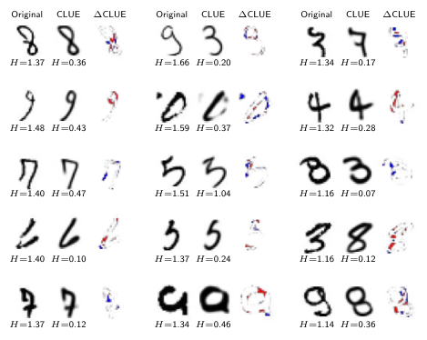
We provide additional examples of CLUEs generated for high uncertainty MNIST digits in Figure 18. U-FIDO counterfactuals generated for the same inputs are shown in Figure 19. Both methods often attribute importance to the same features. However, in almost all cases, CLUE is able to reduce the original input’s uncertainty significantly more than U-FIDO. The latter method suggests smaller changes. We attribute this to U-FIDO’s input masking mechanism being less flexible than CLUE’s latent space generation mechanism.

Appendix H Additional Experimental Results
H.1 Ablation Experiments
In this subsection, we modify some of CLUE’s components individually and observe the effects on the procedure’s results.
Initialization Strategy: Figure 20 compares Algorithm 1’s encoder-based initialization with on all datasets under consideration. For the LSAT, COMPAS and Wine datasets, both approaches produce indistinguishable results. On Credit, our second highest dimensional dataset, using an encoder-based initialization allows for CLUEs to stay slightly closer to original inputs in terms of distance.
The difference between both approaches is largest on MNIST. We conjecture that this might be due to the higher dimensional nature of the latent space used with this dataset making optimization more difficult. By initializing as the VAE encoder’s mean, our optimizer starts near a local minima of and potentially of . When Algorithm 1 is applied, the magnitude of might not be large enough to escape this basin of attraction. Thus, CLUE tends to leave most input features unchanged, only addressing those with most potential to reduce uncertainty. This is also desirable behavior for low uncertainty inputs; the closest low uncertainty sample is the input itself.


Capacity of CLUE’s DGM: To capture our predictive model’s reasoning, CLUE’s DGM must be flexible enough to preserve atypical features in the inputs. As shown in Figure 21, reconstructions from low-capacity VAEs do not preserve the predictive uncertainty of original inputs. The CLUEs generated from these DGMs either leave the inputs unchanged or present large values of while barely reducing : these degenerate CLUEs simply emphasize regions of large reconstruction error. As our DGM’s capacity increases, so does the amount of uncertainty preserved in the auto-encoding operation. The amount of predictive uncertainty explained by CLUEs, which is given by the difference between the autoencoded input uncertainty (orange bars) and CLUE uncertainty (blue bars), increases. We see a clear relationship between dataset dimensionality and size of latent space needed for CLUE to be effective.
Output Space Regularization Parameter : In Figure 22, we show how increasing reduces the proportion of samples for which the predicted class differs between original inputs and CLUEs. Interestingly, on LSAT, Wine and COMPAS, a small, but non-zero, value of results in more uncertainty being explained away by CLUE. However, strongly enforcing similarity of predictions generally comes at the cost of smaller amounts of uncertainty being explained away.
COMPAS predictions stay the same for all values of . Class predictions only depend on 2 of this dataset’s input features (Age and Previous Convictions) (Dressel & Farid 2018). We find that the remaining features can increase or reduce confidence in the prediction given by the two key features, but never change it. CLUEs only change non key features, reinforcing the current classification. On MNIST, we find that, for certain values of , classifying CLUEs results in a lower error rate than classifying original inputs. This is shown in Figure 23. We did not observe this effect for other datasets.
Applying CLUE to non-Bayesian NNs: These models are unable to capture model uncertainty. We train deterministic NNs on every dataset under consideration using the architectures described in Section B.4. We generate counterfactuals for their noise uncertainty. As shown in Figure 24, CLUE is effective at explaining away noise uncertainty for regular NNs. More uncertain inputs are subject to larger changes in terms of distance.


H.2 Verifying Results from our Computational Evaluation Framework
Our computational evaluation framework relies on generating artificial data. There is reasonable concern that the characteristics of this data may not reflect that of real-world data, biasing our results. As explained in Appendix I, we are careful to use powerful g.t. DGM models that generate high quality artificial data. Be that as it may, we validate the results from our computational evaluation framework by performing an analogous informativeness vs relevance experiment on real data.
As we do not have access to the generative process of the real data, we can not exactly quantify the uncertainty of inputs or how in-distribution they are. We instead resort to quantifying informativeness as the amount of our BNN’s predictive uncertainty explained away . We measure relevance as the distance of each counterfactual to its nearest neighbor within the train-set .
We report mean values of , and across all uncertain test points. A test point is deemed to be uncertain according to the criteria outlined in Section B.4. The hyperparameters employed for CLUE also match those provided in Section B.4. The step size used with local sensitivity analysis and U-FIDO’s parameter are found via grid search with a methodology analogous to the one described in Section 5.1.
| Method | LSAT (4) | COMPAS (7) | Wine (11) | ||||||
|---|---|---|---|---|---|---|---|---|---|
| Sensitivity | 0.482 | 0.003 | 0.0192 | 7.975 | 0.265 | 0.033 | 3.317 | 0.481 | 0.154 |
| CLUE | 0.080 | 0.092 | 1.664 | 0.067 | 0.014 | 0.737 | 1.274 | 1.409 | 1.188 |
| U-FIDO | 0.085 | 0.077 | 0.969 | 0.084 | 0.022 | 0.627 | 1.223 | 1.307 | 1.241 |
| Method | Credit (23) | MNIST (784) | ||||
|---|---|---|---|---|---|---|
| Sensitivity | 0.770 | 0.224 | 0.121 | 6.903 | 0.601 | 0.087 |
| CLUE | 1.025 | 0.147 | 0.293 | 4.374 | 0.628 | 0.153 |
| U-FIDO | 1.863 | 0.017 | 0.052 | 4.887 | 0.409 | 0.088 |
As shown in Table 6 and Table 7, CLUE outperforms U-FIDO in terms of on all datasets except wine, where both approaches are very similar. The same is true for the ratio . Like in the artificial data experiments from Section 5.1, the difference between both methods is most stark for high dimensional datasets (MNIST and Credit). Here, CLUE is able to explain away more uncertainty while providing counterfactuals that are similarly close to the training data. Sensitivity is able to greatly reduce uncertainty in high dimensions. However, this comes at the cost going off the data manifold. In low dimensions, there are less possible directions in which steps can be taken, rendering the direct gradient based approach less powerful.
We note that the similarity of these results to the ones obtained in the analogous experiments from Section 5.1 suggest the unbiasedness of our computational evaluation framework.
H.3 Additional Analysis of User Study
While the main text showed the mean accuracy of CLUE over all tabular questions, we also consider the breakdown of accuracy by dataset and by test point certainty in Table 8. CLUE outperforms all baselines on both datasets. We find that sensitivity does significantly worse in higher dimensions (on COMPAS), lending further credence to the intuition described in Appendix D.
When splitting by the certainty of test points, we immediately notice that accuracy for uncertain test points is quite high for all methods. This similarity is expected since certain context points are the only factor that varies between each method’s survey. Survey participants seemed to not use the certain context points to identify uncertain test points. This is probably due to pilot procedure, wherein Participant A carefully paired test points with relevant uncertain context points. Indeed, the random baseline, which controls for the possibility that our task can be solved without access to a relevant counterfactual, performs best on uncertain test points. However, we note a large difference between methods’ results when identifying certain test points. CLUE’s accuracy almost doubles the second best method’s (Human CLUE). When generating Human CLUEs Participant B had knowledge of the uncertain context point, but not the test point (just like other methods). For this reason, we expect to see dissimilarity in methods’ performance on certain test points. CLUE’s ability to bring about most relevant contrast is one possible explanation for why it does so much better than baselines for certain context points.
| Combined | LSAT | COMPAS | Certain Test | Uncertain Test | |
|---|---|---|---|---|---|
| CLUE | |||||
| Human CLUE | |||||
| Random | |||||
| Local Sensitivity |
Appendix I Additional Details on the Generative Model used in the Proposed Computationally Grounded Evaluation Framework
The framework described in Figure 6 uses a conditional DGM, specifically a VAEAC (Ivanov et al. 2019), to both generate artificial data and to evaluate explanations for said data. VAEs are known for generating blurry or overly smoothed data. For our evaluation framework to work well, we require the ground truth DGM to generate sharp data, with atypical characteristic that would to lead to a predictor being uncertain. We can ensure that this is the case by using a large latent dimensionality. However, this brings forth another well-known issue with VAEs: distribution mismatch (Dai & Wipf 2019; Antoran & Miguel 2019; Rosca et al. 2018). The region of latent space where the encoder places probability mass, also known as the aggregate posterior,
does not match the prior .

To visualize this phenomenon, we train a BNN and a VAE on MNIST. We sample points from the VAE’s latent space and evaluate their uncertainty with the BNN. As shown in Figure 25, clusters of same-class digits form in latent space. The aggregate posterior presents low density in the spaces between clusters. Digits generated from these areas are of low-quality, causing our BNN to be uncertain. The outer regions of latent space, where the isotropic Gaussian prior has low density, also generate uncertain digits.
Recently, Dai & Wipf 2019 have proposed the two-level VAE as a solution to distribution mismatch. After training a standard VAE, a second VAE is trained on samples from the first VAE’s latent space. As illustrated in Figure 26, the aggregate posterior over the inner latent variables, which we denote by , more closely resembles the prior. The joint distribution over inputs and latent variables factorizes as: . We refer the reader to (Dai & Wipf 2019) for a detailed analysis. Figure 27 shows that, while generating digits from samples of results in a large amount of low-quality or OOD reconstructions, samples from map to clean digits. The two-stage mechanism restores the VAE’s pivotal ancestral sampling capability, ensuring that our experiments with artificial data will be representative of methods performance on real data.


In order to generate artificial data, we draw samples from the auxiliary latent space, map them back to the VAEAC’s latent space and then map them to the input space. This allows for high-quality sample generation. In this way, a single VAEAC can be used for both ancestral sampling and conditional sampling. In addition, it allows us to estimate the log-likelihood of inputs as:
| (8) |
In Equation 8 parameter subscripts refer to the outer (1st level) and inner (2nd level) networks. In order to preserve computational tractability, we approximate with a point estimate placed at its mean . We further approximate Equation 8 with importance sampling:
| (9) |
I.1 Comparison of Methods under a Ground Truth DGM
The two-level VAEAC setup described above partially addresses the concern that our synthetic data might not be diverse enough to highlight differences among the methods being compared. Indeed, our results from Table 1 and Table 2 show noticeable differences in performance across methods.
We now address the opposite concern; methods that leverage auxiliary VAEs might be unfairly advantaged under our functionally grounded framework, as the generative process of our synthetic data is also VAE-based. Because VAEs are very flexible neural network based generative models, using them as a ground truth provides relatively little inductive biases for auxiliary DGMs to take advantage of. Additionally, our ground truth VAEAC captures the joint distribution of inputs and targets. The metric of interest, , only depends on the conditional distribution over targets . Our auxiliary DGMs only model inputs.
Two of the methods we evaluate, U-FIDO and CLUE, leverage auxiliary DGMs. Thus, both would be equally advantaged. The vs metric from Table 2 is the most dependent on the ground truth VAEAC. However, we observe the largest difference between CLUE and U-FIDO on in this metric.
Appendix J Details on User Study
J.1 Additional Details on Tabular User Study
For our pilot point selection procedure, we take points from each dataset’s test set that score above the uncertainty rejection thresholds described in Section B.4 as uncertain points. Points below the thresholds are labeled as certain points. Pilot procedure participants, referred to as participant A in the main text, were not informed that the pools were split up by the points’ certainty with respect to the BNN being explained.


We now go through the various sections of the main survey. In Figure 28(a), we include the consent form used in our user studies. This user study was performed with the approval of the University of Cambridge’s Department of Engineering Research Ethics Committee. Only three participants who were asked to take the survey did not provide consent and thus exited the form. We still ensured that at least ten participants took each of the four survey variants.


We then include an example question for each dataset, called an “attention check.” An example is shown in Figure 28(b). Note that the answer to this example question is provided in line. Later in the survey, we ask participants this exact same question. We ask one attention check per dataset. If participants get the attention check wrong for both datasets, we void their results. We only had to void one result. This did not affect our criteria of ten completed surveys per variant. The consent form and attention check questions were the same for all survey variants. The main survey participants were first asked the ten LSAT questions followed by the ten COMPAS questions: we made this design decision since the dimensionality of LSAT is lower than that of COMPAS, easing participants into the task. Examples of questions from the CLUE survey variant are shown in Figure 29.
J.2 MNIST User Study
In order to validate CLUE on image data, we create a modified MNIST dataset with clear failure modes for practitioners to identify. We first discard all classes except four, seven, and nine. We then manually identify forty sevens from the training set which have dashes crossing their stems. Using K-nearest-neighbors, we identify the twelve sevens closest to each of the ones manually selected. We delete these 520 sevens from our dataset. We repeat the same procedure for fours which have a closed, triangle-shaped top. We do not delete any digits from the test set. We train a BNN on this new dataset. Our BNN presents high epistemic uncertainty when tested on dashed sevens and closed fours as a consequence of the sparsity of these features in the train set.
We evaluate the test set of fours, sevens, and nines with our BNN. Datapoints that surpass our uncertainty threshold are selected as candidates to be shown in our user study as uncertain context examples or test questions. We show example CLUEs for a four and a seven that display the characteristics of interest in Figure 30.

Leveraging the modified MNIST dataset, we run another user study with questions and two variants. Unlike our tabular experiments, we show practitioners a set of five context points to start, as opposed to a pair. This set of context points is chosen at random from the training set. The first variant involves showing users the set of context points, labeled with if their uncertainty surpasses our predefined threshold. We then ask users to predict if new test points will be certain or uncertain to the BNN. The second variant contains the same labeled context points and test datapoints. However, together with uncertain context points, practitioners are shown CLUEs of how the input features can be changed such that the BNN’s uncertainty falls below the rejection threshold. The practitioners are then asked to decide if new points’ predictions will be certain or not. If CLUE works as intended, practitioners taking the second variant should be able to identify points on which the BNN will be uncertain more accurately.

The first variant was shown to graduate students with machine learning expertise who only received context points and rejection labels (uncertain or not). This group was able to correctly classify of the new test points as high or low uncertainty. The second variant was shown to other graduate students with machine learning expertise who received context points together with CLUEs in cases of high uncertainty. This group was able to reach an accuracy of on new test points. This user study suggests CLUEs are useful for practitioners in image-based settings as well.