IDEAL: Inexact DEcentralized Accelerated Augmented Lagrangian Method
Abstract
We introduce a framework for designing primal methods under the decentralized optimization setting where local functions are smooth and strongly convex. Our approach consists of approximately solving a sequence of sub-problems induced by the accelerated augmented Lagrangian method, thereby providing a systematic way for deriving several well-known decentralized algorithms including EXTRA [41] and SSDA [37]. When coupled with accelerated gradient descent, our framework yields a novel primal algorithm whose convergence rate is optimal and matched by recently derived lower bounds. We provide experimental results that demonstrate the effectiveness of the proposed algorithm on highly ill-conditioned problems.
1 Introduction
Due to their rapidly increasing size, modern datasets are typically collected, stored and manipulated in a distributed manner. This, together with strict privacy requirements, has created a large demand for efficient solvers for the decentralized setting in which models are trained locally at each agent, and only local parameter vectors are shared. This approach has become particularly appealing for applications such as edge computing [42, 25], cooperative multi-agent learning [6, 33] and federated learning [26, 43]. Clearly, the nature of the decentralized setting prevents a global synchronization, as only communication within the neighboring machines is allowed. The goal is then to arrive at a consensus on all local agents with a model that performs as well as in the centralized setting.
Arguably, the simplest approach for addressing decentralized settings is to adapt the vanilla gradient descent method to the underlying network architecture [47, 29, 9, 16]. To this end, the connections between the agents are modeled through a mixing matrix, which dictates how agents average over their neighbors’ parameter vectors. Thus, the mixing matrix serves as a communication oracle which determines how information propagates throughout the network. Perhaps surprisingly, when the stepsizes are constant, simply averaging over the local iterates via the mixing matrix only converges to a neighborhood of the optimum [50, 41]. A recent line of works [40, 15, 41, 34, 30, 31] proposed a number of alternative methods that linearly converge to the global minimum.
The overall complexity of solving decentralized optimization problems is typically determined by two factors: (i) the condition number of the objective function , which measures the ‘hardness’ of solving the underlying optimization problem, and (ii) the condition number of the mixing matrix , which quantifies the severity of information ‘bottlenecks’ present in the network. Lower complexity bounds recently derived for distributed settings [1, 37, 46, 3] show that one cannot expect to have a better dependence on the condition numbers than and . Notably, despite the considerable recent progress, none of the methods mentioned above is able to achieve accelerated rates, that is, a square root dependence for both and —simultaneously.
An extensive effort has been devoted to obtaining acceleration for decentralized algorithms under various settings [37, 38, 22, 48, 51, 45, 14, 10, 11]. When a dual oracle is available, that is, access to the gradients of the dual functions is provided, optimal rates can be attained for smooth and strongly convex objectives [37]. However, having access to a dual oracle is a very restrictive assumption, and resorting to a direct ‘primalization’ through inexact approximation of the dual gradients leads to sub-optimal worst-case theoretical rates [45]. In this work, we propose a novel primal approach that leads to optimal rates in terms of dependency on and .
Our contributions can be summarized as follows.
- •
We introduce a novel framework based on the accelerated augmented Lagrangian method for designing primal decentralized methods. The framework provides a simple and systematic way for deriving several well-known decentralized algorithms [40, 15, 41], including EXTRA [41] and SSDA [37], and unifies their convergence analyses.
- •
Using accelerated gradient descent as a sub-routine, we derive a novel method for smooth and strongly convex local functions which achieves optimal accelerated rates on both the condition numbers of the problem, and , using primal updates, see Table 2.
- •
We perform a large number of experiments, which confirm our theoretical findings, and demonstrate a significant improvement when the objective function is ill-conditioned and .
2 Decentralized Optimization Setting
We consider computational agents and a network graph which defines how the agents are linked. The set of vertices represents the agents and the set of edges specifies the connectivity in the network, i.e., a communication link between agents and exists if and only if . Each agent has access to local information encoded by a loss function . The goal is to minimize the global objective over the entire network,
| (1) |
In this paper, we assume that the local loss functions are differentiable, -smooth and -strongly convex.11 1 is -smooth if is -Lipschitz; is -strongly convex if is convex. Strong convexity of the component functions implies that the problem admits a unique solution, which we denote by .
We consider the following computation and communication models [37]:
- •
Local computation: Each agent is able to compute the gradients of and the cost of this computation is one unit of time.
- •
Communication: Communication is done synchronously, and each agent can only exchange information with its neighbors, where is a neighbor of if . The ratio between the communication cost and computation cost per round is denoted by .
We further assume that propagation of information is governed by a mixing matrix [29, 50, 37]. Specifically, given a local copy of the decision variable at node , one round of communication provides the following update . The following standard assumptions regarding the mixing matrix [37] are made throughout the paper.
Assumption 1.
The mixing matrix satisfies the following:
- 1.
Symmetry: .
- 2.
Positiveness: is positive semi-definite.
- 3.
Decentralized property: If and , then .
- 4.
Spectrum property: The kernel of is given by the vector of all ones .
A typical choice of the mixing matrix is the (weighted) Laplacian matrix of the graph. Another common choice is to set as where is a doubly stochastic matrix [5, 8, 41]. By Assumption 1.4, all the eigenvalues of are strictly positive, except for the smallest one. We let denote the maximum eigenvalue, and let denote the smallest positive eigenvalue. The ratio between these two quantities plays an important role in quantifying the overall complexity of this problem.
Theorem 1 (Decentralized lower bound [37]).
For any first-order black-box decentralized method, the number of time units required to reach an -optimal solution for (1) is lower bounded by
| (2) |
where is the condition number of the loss function and is the condition number of the mixing matrix.
The lower bound decomposes as follows: a) computation cost, given by , and b) communication cost, given by . The computation cost matches lower bounds for centralized settings [32, 2], while the communication cost introduces an additional term which depends on and accounts for the ‘price’ of communication in decentralized models. It follows that the effective condition number of a given decentralized problem is .
Clearly, the choice of the matrix can strongly affect the optimal attainable performance. For example, can get as large as in the line/cycle graph, or be constant in the complete graph. In this paper, we do not focus on optimizing over the choice of for a given graph ; instead, following the approach taken by existing decentralized algorithms, we assume that the graph and the mixing matrix W are given and aim to achieve the optimal complexity (2) for this particular choice of .
3 Related Work and the Dual Formulation
A standard approach to adress problem (1) is to express it as a constrained optimization problem
| (P) |
where is a concatenation of the vectors. To lighten the notation, we introduce the global mixing matrix , where denotes the Kronecker product, and let denote the semi-norm induced by , i.e. . With this notation in hand, we briefly review existing literature on decentralized algorithms.
Decentralized Gradient Descent
The decentralized gradient method [29, 50] has the update rule
| (DGD) |
However, with constant stepsize, the algorithm does not converge to a global minimum of (P), but rather to a neighborhood of the solution [50]. A decreasing stepsize schedule may be used to ensure convergence, but this yields a sublinear convergence rate, even in the strongly convex case.
Input: mixing matrix , regularization parameter , stepsize .
Linearly convergent primal algorithms
By and large, recent methods that achieve linear convergence in the strongly convex case [40, 15, 41, 34, 30, 31, 44] can be shown to follow a general framework based on the augmented Lagrangian method, see Algorithm 1; The main difference lies in how subproblems are solved. Shi et al. 2014 apply an alternating directions method; in [41], the EXTRA algorithm takes a single gradient descent step to solve , see Appendix B for details. Jakovetić et al. 2014a use multi-step algorithms such as Jacobi/Gauss-Seidel methods. To the best of our knowledge, the complexity of these algorithms is not better than , in other words, they are non-accelerated. The recently proposed algorithm APM-C [22] enjoys a square root dependence on and , but incurs an additional factor compared to the optimal attainable rate.
Optimal method based on the dual formulation
By Assumption 1.4, the constraint is equivalent to the identity , which is again equivalent to . Hence, the dual formulation of (P) is given by
| (D) |
Since the primal function is convex and the constraints are linear, we can use strong duality and address the dual problem instead of the primal one. Using this approach, [37] proposed a dual method with optimal accelerated rates, using Nesterov’s accelerated gradient method for the dual problem (D). As mentioned earlier, the main drawback of this method is that it requires access to the gradient of the dual function which, unless the primal function has a relatively simple structure, is not available. One may apply a first-order method to approximate the dual gradients inexactly at the expense of an additional factor in the computation cost [45], but this woul make the algorithm no longer optimal. This indicates that achieving optimal rates when using primal updates is a rather challenging task in the decentralized setting. In the following sections, we provide a generic framework which allows us to derive a primal decentralized method with optimal complexity guarantees.
4 An Inexact Accelerated Augmented Lagrangian framework
Input: mixing matrix , regularization parameter , stepsize , extrapolation parameters
Output: .
Additional Input: A first-order optimization algorithm
Apply to solve the subproblem warm starting at to find an approximate solution
- Option I:
-
stop the algorithm when , where is the unique minimizer of .
- Option II:
-
stop the algorithm after a prefixed number of iterations .
In this section, we introduce our inexact accelerated Augmented Lagrangian framework, and show how to combine it with Nesterov’s acceleration. To ease the presentation, we first describe a conceptual algorithm, Algorithm 2, where subproblems are solved exactly, and only then introduce inexact inner-solvers.
Similarly to Nesterov’s accelerated gradient method, we use an extrapolation step for the dual variable . The component in line 4 of Algorithm 2 is the negative gradient of the Moreau-envelope22 2 A proper definition of the Moreau-envelope is given in [36], readers that are not familiar with this concept could take it as an implicit function which shares the same optimum as the original function. of the dual function. Hence our algorithm is equivalent to applying Nesterov’s method on the Moreau-envelope of the dual function, or equivalently, an accelerated dual proximal point algorithm. This renders the optimal dual method proposed in [37] as a special case of our algorithmic framework (with set to 0).
While Algorithm 2 is conceptually plausible, it requires an exact solution of the Augmented Lagrangian problems, which can be too expensive in practice. To address this issue, we introduce an inexact version, shown in Algorithm 3, where the -th subproblem is solved up to a predefined accuracy . The choice of is rather subtle. On the one hand, choosing a large may result in a non-converging algorithm. On the other hand, choosing a small can be exceedingly expensive as the optimal solution of the subproblem is not the global optimum . Intuitively, should be chosen to be of the same order of magnitude as , leading to the following result.
Theorem 2.
Consider the sequence of primal variables generated by Algorithm 3 with the subproblem solved up to accuracy in Option I. With parameters set to
| (3) |
where , and is the initial dual function gap, we obtain
| (4) |
where and .
Corollary 3.
The number of subproblems to achieve in IDEAL is bounded by
| (5) |
We remark that inexact accelerated Augmented Lagrangian methods have been previously analyzed under different assumptions [28, 19, 49]. The main difference is that here, we are able to establish a linear convergence rate, whereas existing analyses only yield sublinear rates. One of the reasons for this discrepancy is that, although is strongly convex, the dual problem (D) is not, as the mixing matrix is singular. The key to obtaining a linear convergence rate is a fine-grained analysis of the dual problem, showing that the dual variables always lie in the subspace where strong convexity holds. The proof of the theorem relies on the equivalence between Augmented Lagrangian methods and the dual proximal point algorithm [35, 7], which can be interpreted as applying an inexact accelerated proximal point algorithm [13, 23] to the dual problem. A complete convergence analysis is deferred to Section C in the appendix.
Theorem 2 provides an accelerated convergence rate with respect to the ‘augmented’ condition number , as determined by the Augmented Lagrangian parameter in Algorithm 3. We have the following bounds:
| (6) |
where we observe that the condition number is a decreasing function of the regularization parameter . When , the maximum value is attained at , the effective condition number of the decentralized problem. As goes to infinity, the augmented condition number goes to 1. Naively, one may want to take as large as possible to get a fast convergence. However, one must also take into account the complexity of solving the subproblems. Indeed, since is singular, the additional regularization term in does not improve the strong convexity of the subproblems, yielding an increase in inner loops complexity as grows. Hence, the optimal choice of requires balancing the inner and outer complexity in a careful manner.
To study the inner loop complexity, we introduce a warm-start strategy. Intuitively, the distance between and the -th solution to the subproblem is roughly on the order of . More precisely, we have the following result.
Lemma 4.
Given the parameter choice in Theorem 2, initializing the subproblem at yields,
| GD | AGD | SGD | |||
|---|---|---|---|---|---|
Consequently, the ratio between the initial gap at the -th subproblem and the desired gap is bounded by
which is independent of . In other words, the inner loop solver only needs to decrease the iterate gap by a constant factor for each . If the algorithm enjoys a linear convergence rate, a constant number of iteration is sufficient for that. If the algorithm enjoys a sublinear convergence, then the inner loop complexity grows with . To illustrate the behaviour of different algorithms, we present the inner loop complexity for gradient descent (GD), accelerated gradient descent (AGD) and stochastic gradient descent (SGD) in Table 1. Note that while the inner complexity of GD and AGD are independent of , the inner complexity for SGD increases geometrically with . Other possible choices for inner solvers are the alternating directions or Jacobi/Gauss-Seidel method, both of which yield accelerated variants for [40] and [15].
In fact, the theoretical upper bounds on the inner complexity also provide a more practical way to halt the inner optimization processes (see Option II in Algorithm 3). Indeed, one can predefine the computational budget for each subproblem, for instance, iterations of AGD. If this budget exceeds the theoretical inner complexity in Table 1, then the desired accuracy is guaranteed to be reached. In particular, we do not need to evaluate the sub-optimality condition, it is automatically satisfied as long as the budget is chosen appropriately.
Finally, the global complexity is obtained by summing , where is the number of subproblems given in (5). Note that, so far, our analysis applies to any regularization parameter . Since is a function of , this implies that one can select the parameter such that the overall complexity is minimized, leading to the choices of described in Table 1.
Two-fold acceleration
In our setting, acceleration seems to occur in two stages (when compared to the non-accelerated rates in [40, 15, 41, 34, 30]). First, combining IDEAL with GD improves the dependence on the condition of the mixing matrix . Secondly, when used as an inner solver, AGD improves the dependence on the condition number of the local functions . This suggests that the two phenomena are independent; while one is related to the consensus between the agents, as governed by the mixing matrix, the other one is related to the respective centralized hardness of the optimization problem.
Stochastic oracle
Our framework also subsumes the stochastic setting, where only noisy gradients are available. In this case, since SGD is sublinear, the required iteration counters for the subproblem must increase inversely proportional to . Also the stepsize at the -th iteration needs to be decreased accordingly. The overall complexity is now given by . However, in this case, the resulting dependence on the graph condition number can be improved [11].
Multi-stage variant (MIDEAL)
We remark that the complexity presented in Table 2 is abbreviated, in the sense that it does not distinguish between communication cost and computation cost. To provide a more fine-grained analysis, it suffices to note that performing a gradient step of the subproblem requires one local computation to evaluate , and one round of communication to obtain . This implies that when GD/AGD/SGD is combined with IDEAL, the number of local computation rounds is roughly the number of communication rounds, leading to a sub-optimal computation cost, as shown in Table 2.
To achieve optimal accelerated rates, we enforce multiple communication rounds after one evaluation of . This is achieved by substituting the regularization metric with , where is a well-chosen polynomial. In this case, the gradient of the subproblem becomes , which requires rounds of communication.
The choice of the polynomial relies on Chebyshev acceleration, which is introduced in [37, 4]. More concretely, the Chebyshev polynomials are defined by the recursion relation , , , and is defined by
| (7) |
Applying this specific choice of to the mixing matrix reduces its condition number by the maximum amount [37, 4], yielding a graph independent bound . Moreover, the symmetry, positiveness and spectrum property in Assumption 1 are maintained by . Even though no longer satisfies the decentralized property, it can be implemented using rounds of communications with respect to . The implementation details of the resulting algorithm are similar to Algorithm 2, and follow by substituting the mixing matrix by (Algorithm 5 in Appendix E).
| Computation cost | Communication cost | ||||
|---|---|---|---|---|---|
| SSDA+AGD | 0 | ||||
| IDEAL+AGD | |||||
| MSDA+AGD | 0 | ||||
| MIDEAL+AGD |
Comparison with inexact SSDA/MSDA [37]
Recall that SSDA/MSDA are special cases of our algorithmic framework with the degenerate regularization parameter . Therefore, our complexity analysis naturally extends to an inexact anlysis of SSDA/MSDA, as shown in Table 2. although the resulting communication costs are optimal, the computation cost is not, due to the additional factor introduced by solving the subproblems inexactly. In contrast, our multi-stage framework achieves the optimal computation cost.
- •
Low communication cost regime: , the computation cost dominates the communication cost, a improvement is obtained by MIDEAL comparing to MSDA.
- •
Ill conditioned regime: , the complexity of MSDA is dominated by the computation cost while the complexity MIDEAL is dominated by the communication cost . The improvement is proportional to the ratio .
- •
High communication cost regime: , the communication cost dominates, and MIDEAL and MSDA are comparable.
5 Experiments


Having described the IDEAL/MIDEAL algorithms for decentralized optimization problem (1), we now turn to presenting various empirical results which corroborate our theoretical analysis. To facilitate a simple comparison between existing state-of-the-art algorithms, we consider an -regularized logistic regression task over two classes of the MNIST [21] benchmark dataset. The smoohtness parameter (assuming normalized feature vectors) can be shown to be bounded by , which together with a regularization parameter , yields a relatively high -bound on the condition number of the loss function. Further empirical results which demonstrate the robustness of IDEAL/MIDEAL under wide range of parameter choices are provided in Appendix G.
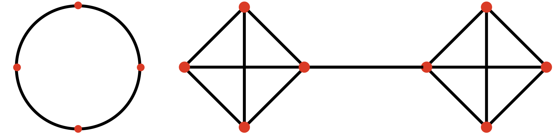
We compare the performance of IDEAL/MIDEAL with the state-of-the-art algorithms EXTRA [41], APM-C [22] and the inexact dual method SSDA/MSDA [37]. We set the inner iteration counter to be for all algorithms, and use the theoretical stepsize schedule. The decentralized environment is modelled in a synthetic setting, where the communication time is steady and no latency is encountered. To demonstrate the effect of the underlying network architecture, we consider: a) a circular graph, where the agents form a cycle; b) a Barbell graph, where the agents are split into two complete subgraphs, connected by a single bridge (shown in Figure 2 in the appendix).
As shown in Figure 1, our multi-stage algorithm MIDEAL is optimal in the regime where the communication cost is small, and the single-stage variant IDEAL is optimal when is large. As expected, the inexactness mechanism significantly slows down the dual method SSDA/MSDA in the low communication cost regime. In contrast, the APM-C algorithm performs reasonably well in the low communication regime, but performs relatively poorly when the communication cost is high.
6 Conclusions
We propose a novel framework of decentralized algorithms for smooth and strongly convex objectives. The framework provides a unified viewpoint of several well-known decentralized algorithms and, when instantiated with AGD, achieves optimal convergence rates in theory and state-of-the-art performance in practice. We leave further generalization to (non-strongly) convex and non-smooth objectives to future work.
Acknowledgements
YA and JB acknowledge support from the Sloan Foundation and Samsung Research. BC and MG acknowledge support from the grants NSF DMS-1723085 and NSF CCF-1814888. HL and SJ acknowledge support by The Defense Advanced Research Projects Agency (grant number YFA17 N66001-17-1-4039). The views, opinions, and/or findings contained in this article are those of the author and should not be interpreted as representing the official views or policies, either expressed or implied, of the Defense Advanced Research Projects Agency or the Department of Defense.
Broader impact
Centralization of data is not always possible because of security and legacy concerns [12]. Our work proposes a new optimization algorithm in the decentralized setting, which can learn a model without revealing the privacy sensitive data. Potential applications include data coming from healthcare, environment, safety, etc, such as personal medical information [17, 18], keyboard input history [27, 20] and beyond.
References
- Arjevani and Shamir [2015] Y. Arjevani and O. Shamir. Communication complexity of distributed convex learning and optimization. In Proceedings of Advances in Neural Information Processing Systems (NIPS), 2015.
- Arjevani and Shamir [2016] Y. Arjevani and O. Shamir. On the iteration complexity of oblivious first-order optimization algorithms. In International Conferences on Machine Learning (ICML), 2016.
- Arjevani et al. [2020] Y. Arjevani, O. Shamir, and N. Srebro. A tight convergence analysis for stochastic gradient descent with delayed updates. In Proceedings of the 31st International Conference on Algorithmic Learning Theory, volume 117, pages 111–132, 2020.
- Auzinger and Melenk [2011] W. Auzinger and J. Melenk. Iterative solution of large linear systems. Lecture Note, 2011.
- Aybat and Gürbüzbalaban [2017] N. S. Aybat and M. Gürbüzbalaban. Decentralized computation of effective resistances and acceleration of consensus algorithms. In 2017 IEEE Global Conference on Signal and Information Processing (GlobalSIP), pages 538–542. IEEE, 2017.
- Bernstein et al. [2002] D. S. Bernstein, R. Givan, N. Immerman, and S. Zilberstein. The complexity of decentralized control of markov decision processes. Mathematics of operations research, 27(4):819–840, 2002.
- Bertsekas [2014] D. P. Bertsekas. Constrained optimization and Lagrange multiplier methods. Academic press, 2014.
- Can et al. [2019] B. Can, S. Soori, N. S. Aybat, M. M. Dehvani, and M. Gürbüzbalaban. Decentralized computation of effective resistances and acceleration of distributed optimization algorithms. arXiv preprint arXiv:1907.13110, 2019.
- Duchi et al. [2011] J. C. Duchi, A. Agarwal, and M. J. Wainwright. Dual averaging for distributed optimization: Convergence analysis and network scaling. IEEE Transactions on Automatic control, 57(3):592–606, 2011.
- Dvinskikh and Gasnikov [2019] D. Dvinskikh and A. Gasnikov. Decentralized and parallelized primal and dual accelerated methods for stochastic convex programming problems. arXiv preprint arXiv:1904.09015, 2019.
- Fallah et al. [2019] A. Fallah, M. Gürbüzbalaban, A. Ozdaglar, U. Simsekli, and L. Zhu. Robust distributed accelerated stochastic gradient methods for multi-agent networks. arXiv preprint arXiv:1910.08701, 2019.
- GDPR [2016] GDPR. The eu general data protection regulation (gdpr). 2016.
- Güler [1992] O. Güler. New proximal point algorithms for convex minimization. SIAM Journal on Optimization, 2(4):649–664, 1992.
- Hendrikx et al. [2020] H. Hendrikx, F. Bach, and L. Massoulie. An optimal algorithm for decentralized finite sum optimization, 2020.
- Jakovetić et al. [2014a] D. Jakovetić, J. M. Moura, and J. Xavier. Linear convergence rate of a class of distributed augmented lagrangian algorithms. IEEE Transactions on Automatic Control, 60(4):922–936, 2014a.
- Jakovetić et al. [2014b] D. Jakovetić, J. Xavier, and J. M. Moura. Fast distributed gradient methods. IEEE Transactions on Automatic Control, 59(5):1131–1146, 2014b.
- Jochems et al. [2016] A. Jochems, T. M. Deist, J. Van Soest, M. Eble, P. Bulens, P. Coucke, W. Dries, P. Lambin, and A. Dekker. Distributed learning: developing a predictive model based on data from multiple hospitals without data leaving the hospital–a real life proof of concept. Radiotherapy and Oncology, 121(3):459–467, 2016.
- Jochems et al. [2017] A. Jochems, T. M. Deist, I. El Naqa, M. Kessler, C. Mayo, J. Reeves, S. Jolly, M. Matuszak, R. Ten Haken, J. van Soest, et al. Developing and validating a survival prediction model for nsclc patients through distributed learning across 3 countries. International Journal of Radiation Oncology* Biology* Physics, 99(2):344–352, 2017.
- Kang et al. [2015] M. Kang, M. Kang, and M. Jung. Inexact accelerated augmented lagrangian methods. Computational Optimization and Applications, 62(2):373–404, 2015.
- Konecný et al. [2016] J. Konecný, H. B. McMahan, F. X. Yu, P. Richtarik, A. T. Suresh, and D. Bacon. Federated learning: Strategies for improving communication efficiency. In NIPS Workshop on Private Multi-Party Machine Learning, 2016. URL https://arxiv.org/abs/1610.05492.
- LeCun et al. [2010] Y. LeCun, C. Cortes, and C. Burges. Mnist handwritten digit database. ATT Labs [Online], 2, 2010. URL http://yann.lecun.com/exdb/mnist.
- Li et al. [2018] H. Li, C. Fang, W. Yin, and Z. Lin. A sharp convergence rate analysis for distributed accelerated gradient methods. arXiv preprint arXiv:1810.01053, 2018.
- Lin et al. [2017] H. Lin, J. Mairal, and Z. Harchaoui. Catalyst acceleration for first-order convex optimization: from theory to practice. The Journal of Machine Learning Research, 18(1):7854–7907, 2017.
- Mairal [2016] J. Mairal. End-to-end kernel learning with supervised convolutional kernel networks. In Proceedings of Advances in Neural Information Processing Systems (NIPS), 2016.
- Mao et al. [2017] Y. Mao, C. You, J. Zhang, K. Huang, and K. B. Letaief. A survey on mobile edge computing: The communication perspective. IEEE Communications Surveys & Tutorials, 19(4):2322–2358, 2017.
- McMahan et al. [2017] B. McMahan, E. Moore, D. Ramage, S. Hampson, and B. A. y Arcas. Communication-efficient learning of deep networks from decentralized data. In Artificial Intelligence and Statistics, pages 1273–1282, 2017.
- McMahan et al. [2016] H. B. McMahan, E. Moore, D. Ramage, S. Hampson, et al. Communication-efficient learning of deep networks from decentralized data. arXiv preprint arXiv:1602.05629, 2016.
- Nedelcu et al. [2014] V. Nedelcu, I. Necoara, and Q. Tran-Dinh. Computational complexity of inexact gradient augmented lagrangian methods: application to constrained mpc. SIAM Journal on Control and Optimization, 52(5):3109–3134, 2014.
- Nedic and Ozdaglar [2009] A. Nedic and A. Ozdaglar. Distributed subgradient methods for multi-agent optimization. IEEE Transactions on Automatic Control, 54(1):48–61, 2009.
- Nedic et al. [2017] A. Nedic, A. Olshevsky, and W. Shi. Achieving geometric convergence for distributed optimization over time-varying graphs. SIAM Journal on Optimization, 27(4):2597–2633, 2017.
- Nedić et al. [2017] A. Nedić, A. Olshevsky, W. Shi, and C. A. Uribe. Geometrically convergent distributed optimization with uncoordinated step-sizes. In 2017 American Control Conference (ACC), pages 3950–3955. IEEE, 2017.
- Nesterov [2004] Y. Nesterov. Introductory lectures on convex optimization, volume 87. Springer Science & Business Media, 2004.
- Panait and Luke [2005] L. Panait and S. Luke. Cooperative multi-agent learning: The state of the art. Autonomous agents and multi-agent systems, 11(3):387–434, 2005.
- Qu and Li [2017] G. Qu and N. Li. Harnessing smoothness to accelerate distributed optimization. IEEE Transactions on Control of Network Systems, 5(3):1245–1260, 2017.
- Rockafellar [1976] R. T. Rockafellar. Augmented lagrangians and applications of the proximal point algorithm in convex programming. Mathematics of operations research, 1(2):97–116, 1976.
- Rockafellar and Wets [2009] R. T. Rockafellar and R. J.-B. Wets. Variational analysis, volume 317. Springer Science & Business Media, 2009.
- Scaman et al. [2017] K. Scaman, F. Bach, S. Bubeck, Y. T. Lee, and L. Massoulié. Optimal algorithms for smooth and strongly convex distributed optimization in networks. In International Conferences on Machine Learning (ICML), 2017.
- Scaman et al. [2018] K. Scaman, F. Bach, S. Bubeck, L. Massoulié, and Y. T. Lee. Optimal algorithms for non-smooth distributed optimization in networks. In Proceedings of Advances in Neural Information Processing Systems (NIPS), 2018.
- Schmidt et al. [2011] M. Schmidt, N. L. Roux, and F. R. Bach. Convergence rates of inexact proximal-gradient methods for convex optimization. In Proceedings of Advances in Neural Information Processing Systems (NIPS), 2011.
- Shi et al. [2014] W. Shi, Q. Ling, K. Yuan, G. Wu, and W. Yin. On the linear convergence of the ADMM in decentralized consensus optimization. IEEE Transactions on Signal Processing, 62(7):1750–1761, 2014.
- Shi et al. [2015] W. Shi, Q. Ling, G. Wu, and W. Yin. Extra: An exact first-order algorithm for decentralized consensus optimization. SIAM Journal on Optimization, 25(2):944–966, 2015.
- Shi et al. [2016] W. Shi, J. Cao, Q. Zhang, Y. Li, and L. Xu. Edge computing: Vision and challenges. IEEE internet of things journal, 3(5):637–646, 2016.
- Shokri and Shmatikov [2015] R. Shokri and V. Shmatikov. Privacy-preserving deep learning. In Proceedings of the 22nd ACM SIGSAC conference on computer and communications security, pages 1310–1321, 2015.
- Sun et al. [2019] Y. Sun, A. Daneshmand, and G. Scutari. Convergence rate of distributed optimization algorithms based on gradient tracking. arXiv preprint arXiv:1905.02637, 2019.
- Uribe et al. [2020] C. A. Uribe, S. Lee, A. Gasnikov, and A. Nedić. A dual approach for optimal algorithms in distributed optimization over networks. Optimization Methods and Software, pages 1–40, 2020.
- Woodworth et al. [2018] B. E. Woodworth, J. Wang, A. Smith, B. McMahan, and N. Srebro. Graph oracle models, lower bounds, and gaps for parallel stochastic optimization. In Proceedings of Advances in Neural Information Processing Systems (NIPS), 2018.
- Xiao et al. [2007] L. Xiao, S. Boyd, and S.-J. Kim. Distributed average consensus with least-mean-square deviation. Journal of parallel and distributed computing, 67(1):33–46, 2007.
- Xu et al. [2020] J. Xu, Y. Tian, Y. Sun, and G. Scutari. Accelerated primal-dual algorithms for distributed smooth convex optimization over networks. International Conference on Artificial Intelligence and Statistics (AISTATS), 2020.
- Yan and He [2020] S. Yan and N. He. Bregman augmented lagrangian and its acceleration, 2020.
- Yuan et al. [2016] K. Yuan, Q. Ling, and W. Yin. On the convergence of decentralized gradient descent. SIAM Journal on Optimization, 26(3):1835–1854, 2016.
- Zhang et al. [2019] J. Zhang, C. A. Uribe, A. Mokhtari, and A. Jadbabaie. Achieving acceleration in distributed optimization via direct discretization of the heavy-ball ode. In 2019 American Control Conference (ACC), pages 3408–3413. IEEE, 2019.
Appendix A Remark on the choice of the mixing matrix
In the main paper, the mixing matrix is defined following the convention used in [37], where the kernel of is the vector of all ones. It is worth noting that the term mixing matrix is also used in the literature to denote a doubly stochastic matrix (see e.g. [40, 15, 41, 34, 30, 31, 8]). These two approaches are equivalent as given a doubly stochastic matrix , the matrix
In the following discussion, we will use to draw the connection when necessary.
Appendix B Recovering EXTRA under the augmented Lagrangian framework
The goal of this section is to show that EXTRA algorithm [41] is a special case of the non-accelerated Augmented Lagrangian framework in Algorithm 1.
Proposition 5.
The EXTRA algorithm is equivalent to applying one step of gradient descent to solve the subproblem in Algorithm 1.
Proof.
Remark 6.
When expressing the parameters in terms of , the inner loop stepsize reads as , and the outer-loop stepsize reads as .
Appendix C Proof of Theorem 3
Input: mixing matrix , regularization parameter , stepsize , extrapolation parameters
Output: .
We start by noting that Algorithm 2 is equivalent to the “unscaled" version of Algorithm 4. More specifically, we recover Algorithm 2 by substituting the variables
The unscaled version is computationally inefficient since it requires the computation of the square root of . This is the reason why we choose to present the scaled version Algorithm 2 in the main paper. However, the unscaled version is easier to work with for the analysis. In the following proof, the variables and are referred to as in the unscaled version Algorithm 4.
The key concept underlying our analysis on is the Moreau-envelope of the dual problem:
| (10) |
Similarly, we define the associated proximal operator
| (11) |
Note that when the inner problem is strongly convex, the proximal operator is unique (that is, a single-valued operator). The following is a list well known properties of the Moreau-envelope:
Proposition 7.
The Moreau envelope enjoys the following properties
- 1.
is convex and it shares the same optimum as the dual problem (D).
- 2.
is differentiable and the gradient of is given by
- 3.
If is twice differentiable, then its convex conjugate is also twice differentiable. In this case, is also twice differentiable and the Hessian is given by
Corollary 8.
The Moreau envelope satisfies
- 1.
is -smooth, where .
- 2.
is -strongly convex in the image space of , where .
Proof.
These properties follow from the expressions for the Hessian of and by the fact that is -smooth and strongly convex. ∎
In particular, is only strongly convex on the image space of , one of the keys to prove the linear convergence rate is the following lemma.
Lemma 9.
The variables and in the un-scaled version Algorithm 4 all lie in the image space of for any .
Proof.
This can be easily derived by induction according to the update rule in line 4, 5 of Algorithm 4. ∎
Similar to the dual Moreau-envelope, we also define the weighted Moreau-envelope on the primal function
| (12) |
and its associated proximal operator
| (13) |
Indeed, this function corresponds exactly to the subproblem solved in the augmented Lagrangian framework (line 3 of Algorithm 2). Similar property holds for :
Proposition 10.
The Moreau envelope enjoys the following properties:
- 1.
is concave.
- 2.
is differentiable and the gradient of is given by
- 3.
If is twice differentiable, then is also twice differentiable and the Hessian is given by
In particular, is -smooth and strongly concave.
The dual Moreau-envelope and primal Moreau-envelope are connected through the following relationship.
Proposition 11.
The gradient of the Moreau envelope is given by
| (14) |
Proof.
Proposition 14 demonstrates that solving the augmented Lagrangian subproblem could be viewed as evaluating the gradient of the Moreau-envelope. Hence applying gradient descent on the Moreau-envelope gives the non-accelerated augmented Lagrangian framework Algorithm 1. Even more, applying Nesterov’s accelerated gradient on the Moreau-envelope yields accelerated Augmented Lagrangian Algorithm 4. In addition, when the subproblems are solved inexactly, this corresponds to an inexact evaluation on the gradient. This interpretation allows us to derive guarantees for the convergence rate of the dual variables. Before present the the convergence analysis in detail, we formally establish the connection between the primal solution and the dual solution.
Lemma 12.
Let be the optimum of and define . Then there exists a unique such that is the optimum of the dual problem (D). Moreover, it satisfies
Proof.
Since , we have
where is the canonical basis with all entries 0 except the -th equals to 1. By optimality, . This implies that , for all . In other words, is orthogonal to the null space of , namely . Therefore, there exists such that . By setting , we have and . In particular, since , we have,
| (15) |
Hence is the solution of the dual problem (D) and it is the unique one lies in the . ∎
Throughout the rest of the paper, we use to denote the unique solution as shown in the lemma above. We would like to emphasize that even though is strongly convex, the dual problem (D) is not strongly convex, because is singular. Hence, the solution of the dual problem is not unique unless we restrict to the image space of . To derive the linear convergence rate, we need to show that the dual variable always lies in this subspace where the Moreau-envelope is strongly convex.
Theorem 13.
Consider the sequence of primal variables generated by Algorithm 3 with the subproblem solved up to accuracy, i.e. Option I. Therefore,
| (16) |
where , , , , is the dual function gap defined by and
Proof.
The proof builds on the concepts developed so far in this section. We start by showing that the dual variable converges to the dual solution in a linear rate. From the interpretation given in Prop 7 and Prop 11, the sequence given in Algorithm 2 is equivalent to applying Nesterov’s accelerated gradient method on the Moreau-envelope . In the inexact variant, the inexactness on the solution directly translates to an inexact gradient of , where the inexactness is given by
Hence in Algorithm 4 is obtained by applying inexact accelerated gradient method on the Moreau-envelope . Note that by induction and belong to the image space of , in which the dual Moreau-envelope is strongly convex. Following the analysis on inexact accelerated gradient method Prop 4 in [39], we have
| (17) |
where and is the accumulation of the errors given by
Based on the convergence on the dual variable, we could now derive the convergence on the primal variable. Let be the exact solution of the problem . Then
| (18) |
Finally, from triangle inequality
The desired inequality follows from reorganizing the constant and the fact that . ∎
Appendix D Proof of Lemma 4
Lemma 14.
With the parameter choice as Theorem 2, then warm starting the -th subproblem at the previous solution gives an initial gap
Proof.
From triangle inequality, we have
The desired inequality follows from the convergence on the primal iterates and (C), i.e.
∎
Appendix E Multi-stage algorithm: MIDEAL
Input: mixing matrix , regularization parameter , stepsize , extrapolation parameters
Output: .
Input: mixing matrix , vector or matrix .
Output: .
Intuitively, we simply replace the mixing matrix by , resulting in a better graph condition number. However, each evaluation of the new mixing matrix requires rounds of communication, given by the AcceleratedGossip algorithm introduced in [37]. For completeness of the discussion, we recall this procedure in Algorithm 6. In particular, given and , AcceleratedGossip(,) returns , based on the communication oracle .
Appendix F Implementation of Algorithms
Input: number of iterations , gossip matrix
Output:
Appendix G Further Experimental Results