Impedances and Instabilities

Consider a point charge $q$ moving in free space at a velocity $v$ close to the speed of light. The electromagnetic field is Lorentz-contracted into a thin disk perpendicular to the particle’s direction of motion [7], which we choose to be the $z$-axis in a cylindrical coordinate system. The opening angle of the field distribution is of the order of $1/\gamma$, where $\gamma={(1-{(v/c)}^{2})}^{-1/2}$. The field distribution is shown in Fig. 1. Even for an electron beam with an energy of $E=10\>{\rm MeV}$, the opening angle $\phi$ is no greater than $50\>{\rm mrad}$ or $2.89^{\circ}$:

($m_{0}c^{2}=0.511\,{\rm MeV}$ is the rest mass of the electron).

In the ultra-relativistic limit $v\rightarrow c$ (or $\gamma\rightarrow\infty$), the disk containing the field shrinks to a $\delta$-function distribution. The non-vanishing field components are

Since the electric field $\hskip-2.84526ptE\hskip-2.84526pt$ points strictly radially outward from the point charge, all field components are identically zero both ahead of and behind the point charge, and hence there are no forces on a test particle either preceding or following the charge $q$.

For $v$ slightly less than $c$, this is not strictly true. However, if we look at some typical bunch charges and energies of high-energy accelerators and synchrotron light sources, as shown in Table 1, we will notice that the space charge force $V_{\rm s}=e/(4\,\pi\,\epsilon_{0}\,d^{2}\,\gamma^{2})$ (where $d$ is the rms distance between two electrons in the bunch) scales with $1/\gamma^{2}$. It is then obvious that as a good approximation, any space charge effects can be neglected for the accelerators under consideration. Nevertheless, space charge effects are important in heavy ion or low-energy proton accelerators.

In the next section we will restrict ourselves to the ultra-relativistic case ($\gamma=\infty,\,v=c$), so space charge effects are neglected.

Consider some typical settings where electromagnetic fields occur behind a bunch with charge $q$ moving with velocity $c$ through a structure. A bunch moves through a cylindrical pipe along the $z$-axis. All electric field lines terminate transversely on surface charges on the wall of the pipe, assuming a perfectly conducting wall. There will be no wake fields behind the charge. The situation is different, however, if the cross-section of the beam pipe changes. A step-out transition is shown in Fig. 2. All fields have been calculated using a numerical wake field solver from MAFIA or the CST studio suite [13, 14, 11, 12].

Here we have assumed that all pipe walls are perfect conductors. The wake field is generated because of the change in geometry. It should be noted that any beam pipe with finite conductivity, as well as flat beam pipes, can generate wake fields (resistive wall wake fields) [15]. Furthermore, a dielectric-coated pipe, which could be used as a travelling-wave acceleration section, will generate wake fields; see, for example, [16].

Another example is a cavity in a beam pipe; see Fig. 3. Again, a bunch is moving through a cylindrical pipe along the $z$-axis. Wake fields are generated because of geometrical changes in the pipe cross-section. In this respect the situation is similar to the previously considered case of a step-out transition. The main difference is that the bunch can excite modes in the cavity and therefore long-range wake fields, which can ring for a long time in the cavity (depending on the conductivity of the cavity wall).

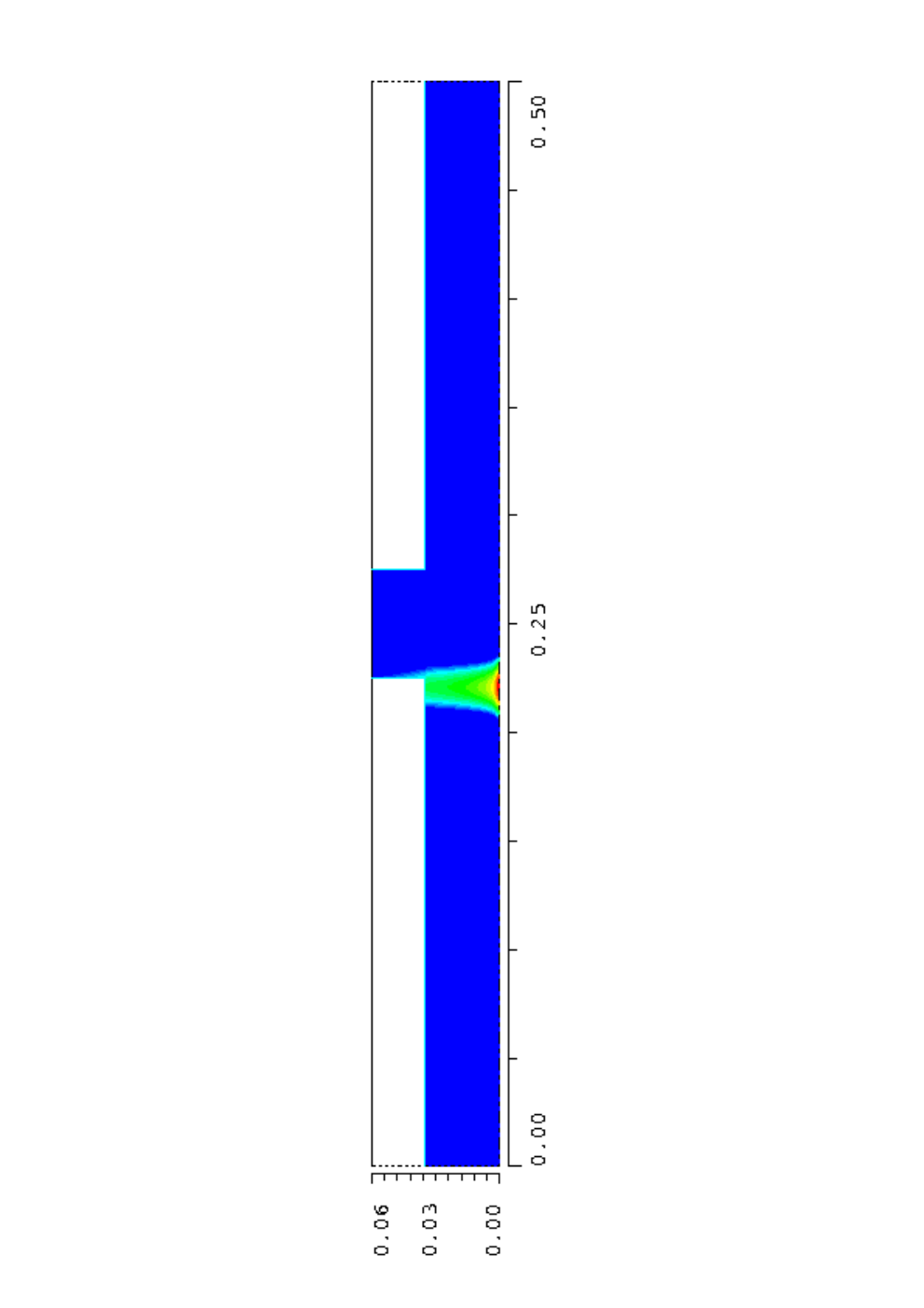
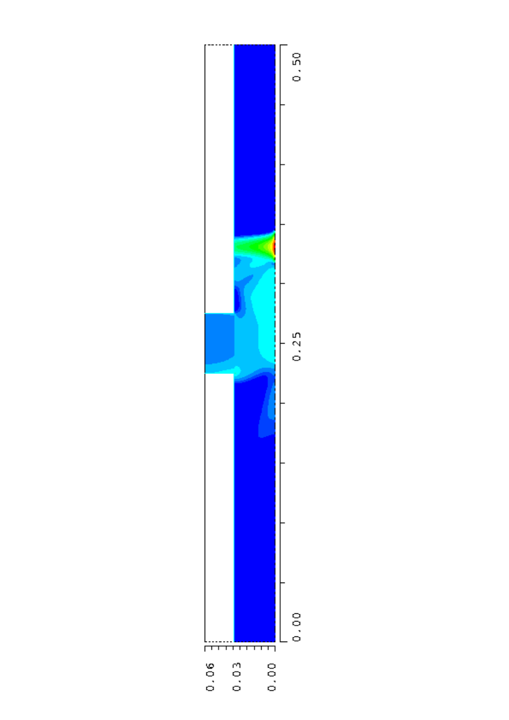
The examples have demonstrates that wake forces are caused by geometrical changes along the beam pipe. Space charge effects are negligible for ultra-relativistic particles. Wake fields due to the resistive wall or dielectric coatings should always be checked in detail according to the specific situation. Furthermore, the surface roughness of the vacuum chamber can be important for special cases [17].

The examples above give us a qualitative understanding of wake fields and how they are generated. Before proceeding to mathematical descriptions in terms of wake potentials, let us take a closer look at the example considered in Section 1.

An ultra-relativistic point particle with charge $q_{1}$ traverses a small cavity parallel to the $z$-axis, with offset $(x_{1},y_{1})$; see Fig. 4.

The electromagnetic force on any test charge $q_{2}$ is given as a function of space and time coordinates by the Lorentz equation

where $\hskip-2.84526ptE\hskip-2.84526pt$ and $\hskip-2.84526ptB\hskip-2.84526pt$ are the fields generated by $q_{1}$; they are solutions of the Maxwell equations {alignat*}4 $\hskip-2.84526pt\nabla\hskip-2.84526pt$ × $\hskip-2.84526ptB\hskip-2.84526pt$ = μ_0 $\hskip-2.84526ptj\hskip-2.84526pt$ + 1 c 2 ∂ ∂t $\hskip-2.84526ptE\hskip-2.84526pt$ ,    $\hskip-2.84526pt\nabla\hskip-2.84526pt$ ⋅ $\hskip-2.84526ptB\hskip-2.84526pt$ = 0,
$\hskip-2.84526pt\nabla\hskip-2.84526pt$ × $\hskip-2.84526ptE\hskip-2.84526pt$ = - ∂ ∂t $\hskip-2.84526ptB\hskip-2.84526pt$ ,    $\hskip-2.84526pt\nabla\hskip-2.84526pt$ ⋅ $\hskip-2.84526ptE\hskip-2.84526pt$ = 1 ϵ 0 ρ and have to satisfy several boundary conditions.

In our case the charge and current distributions are

After interaction of $q_{1}$ with the cavity, there remain electromagnetic fields in the cavity. The source particle has lost energy to cavity modes and excited fields that propagate in the semi-infinite beam pipes.

Now consider a test charge $q_{2}$ following $q_{1}$ at a distance $s$ with the same velocity $v\approx c$ and with offset $(x_{2},y_{2})$. The Lorentz force is

The change in momentum of the test charge can be calculated as the time-integrated Lorentz force,

This leads to the concept of wake functions.

The electromagnetic fields $\mbox{ \boldmath$\hskip-2.84526ptE\hskip-2.84526pt$ }_{\rm d}$ and $\mbox{ \boldmath$\hskip-2.84526ptB\hskip-2.84526pt$ }_{\rm d}$ and the Lorentz Force $\mbox{ \boldmath$\hskip-2.84526ptF\hskip-2.84526pt$ }_{\rm d}$ of a distributed source $\rho_{\rm d}(\mbox{ \boldmath$\hskip-2.84526ptr\hskip-2.84526pt$ },t)=\eta(x_{1}-{\bar{x}}_{1},y_{1}-{\bar{y}}_{1})\lambda(z-ct)$ can be calculated either by integration over all source points,

or by solving the electromagnetic problem for the distributed source; here $\lambda$ is the line charge density, $\eta$ is the transverse distribution normalized to 1, and ${\bar{x}}_{1}$ and ${\bar{y}}_{1}$ describe a transverse shift of the center of the distribution. A calculation of the electric fields of a distributed source is shown in Fig. 5.

A fundamental difference between fields of point particles (with time dependency $\delta(z-ct)$) and fields of distributed sources (with time dependency $\lambda(z-ct)$) is that the frequency spectrum of point particles is not limited. In particular, long Gaussian bunches may stimulate only a few resonances (modes) in a cavity structure, or even none.

We can distinguish between the long-range regime of the wake, where the interaction between particles is driven by resonances, and the short-range regime, where the superposition of time-harmonic cavity fields is not sufficient to describe the effects. For instance, the fields in Fig. 2 are not determined by oscillations, while the fields in Fig. 5 will ring harmonically on one or several frequencies after the (source) bunch has left the domain.

Consider a point charge $q_{1}$ traversing a structure with offset $(x_{1},y_{1})$ parallel to the $z$-axis at the speed of light (see Fig. 4). Then the wake function is defined as

The distance $s$ is measured from the source $q_{1}$ in the opposite direction to $\hskip-2.84526ptv\hskip-2.84526pt$ . The change in momentum of a test particle with charge $q_{2}$ following behind at a distance $s$ with offset $(x_{2},y_{2})$ is given by

Since $\mbox{ \boldmath$\hskip-2.84526pte_{z}\hskip-2.84526pt$ }\cdot(\mbox{ \boldmath$\hskip-2.84526pte_{z}\hskip-2.84526pt$ }\times\mbox{ \boldmath$\hskip-2.84526ptB\hskip-2.84526pt$ })=0$, the longitudinal component of the wake function is simply

Figure 6 shows the longitudinal component of the wake potential for the above example with the small cavity. The grey line represents the Gaussian charge distribution in the range from $-5\sigma$ to $10\sigma$. Owing to transient wake field effects, the head of the bunch (left-hand side of the figure) is decelerated, while a test charge at a certain position behind the bunch will be accelerated.

The notion of wakes, as presented above, is restricted to sources and test particles that travel at the velocity of light through a structure with semi-infinite input and output beam pipes. Therefore, for the integrals to converge, it is necessary that there be no length-independent forces in the pure beam pipes. This is the case for $v\rightarrow c$ and perfect conductivity of the pipes. The concept of a wake per length,

is used to describe the effect in beam pipes ‘p’ of finite conductivity and/or velocity $v\leq c$. Suppose that the input and output beam pipes have the same cross-section; then a generalized wake function

can be defined for the scattered fields $\mbox{ \boldmath$\hskip-2.84526ptE\hskip-2.84526pt$ }_{\rm s}=\mbox{ \boldmath$\hskip-2.84526ptE\hskip-2.84526pt$ }-\mbox{ \boldmath$\hskip-2.84526ptE\hskip-2.84526pt$ }_{\rm p}$ and $\mbox{ \boldmath$\hskip-2.84526ptB\hskip-2.84526pt$ }_{\rm s}=\mbox{ \boldmath$\hskip-2.84526ptB\hskip-2.84526pt$ }-\mbox{ \boldmath$\hskip-2.84526ptB\hskip-2.84526pt$ }_{\rm p}$. If the conditions for the wake function are fulfilled (i.e. convergence of the integral), then the wake function equals the generalized wake function.

The wake potential is defined similarly to the wake function, but for a distributed source: {align*} $\hskip-2.84526ptW\hskip-2.84526pt$ ( ¯ x _1, ¯ y _1,x_2,y_2,s) = 1 q 1 ∫_-∞^∞ dz  [ $\hskip-2.84526ptE\hskip-2.84526pt$ _d(x_2,y_2,z,t) + c   $\hskip-2.84526pte\hskip-2.84526pt$ _z × $\hskip-2.84526ptB\hskip-2.84526pt$ _d(x_2,y_2,z,t) ] _t=(s+z)/ c
= 1 q 1 q 2 ∫_-∞^∞ dz  [ $\hskip-2.84526ptF\hskip-2.84526pt$ _d( ¯ x _1, ¯ y _1,x_2,y_2,z,t) ] _t=(s+z)/ c. It can be calculated from the wake function by the convolution

Note that the $s$-coordinate measures in the negative $z$-direction while $\lambda$ depends on the positive longitudinal coordinate. Usually numerical codes for computing wakes, such as ECHO, calculate electromagnetic fields for distributed sources and therefore wake potentials.

Consider now a cylindrically symmetric acceleration cavity with side tubes of radius $a$ (see Fig. 7). The particular shape in the region $r>a$ is of no importance for the following investigations. Two charges pass through the structure from left to right with the speed of light: $q_{1}$ at a radius of $r_{1}$ and $q_{2}$ at a radius of $r_{2}$. We wish to find an expression for the net change in momentum, $\Delta\mbox{ \boldmath$\hskip-2.84526ptp\hskip-2.84526pt$ }(r_{1},\varphi_{1},r_{2},\varphi_{2},s)$, experienced by $q_{2}$ due to the wake fields generated by $q_{1}$. In the following we write the wake function and potential in polar coordinates. Let us start with the case of $\varphi_{1}=0$:

The wake function can be expanded in a multipole series

Since $w_{\|}$ is a harmonic function in $(r_{2},\varphi_{2})$, we have {align*} L_2  w_∥(r_1,0,r_2,φ_2,s) = ( 1 r 2 ∂ ∂r 2 r_2 ∂ ∂r 2 + 1 r 2 ∂ 2 ∂φ 2 2 ) w_∥(r_1,0,r_2,φ_2,s)
= Re { ∑_m=-∞^∞ exp(i  m   φ_2) ( 1 r 2 ∂ ∂r 2 r_2 ∂ ∂r 2 - m 2 r 2 2 ) G_m(r_1,r_2,s) }
= 0, where $L_{2}$ is the transverse Laplace operator with respect to the offset of the test particle. So, for all $m$, the expansion functions $G_{m}(r_{1},r_{2},s)$ have to satisfy the Poisson equation

The solutions are {align*} G_0(r_1,r_2,s) = U_0(r_1,s) + V_0(r_1,s)   lnr_2,
G_m(r_1,r_2,s) = U_m(r_1,s)   r_2^m + V_m(r_1,s)   r_2^-m  \textfor m > 0.

Keeping only the solutions which are regular at the origin ($r_{2}=0$), the longitudinal wake potential can be written as

with expansion functions $U_{m}(r_{1},s)$ that depend on the details of the given cavity geometry.

By azimuthal symmetry, the dependence on $\varphi_{1}$ is $w_{\|}(r_{1},\varphi_{1},r_{2},\varphi_{2},s)=w_{\|}(r_{1},0,r_{2},\varphi_{2}-\varphi_{2},s)$, as longitudinal fields depend only on the relative azimuthal angle of the observer with respect to the source. Using the fact that $w_{\|}$ is also a harmonic function in $(r_{1},\varphi_{1})$, we find with the same arguments as before that $U_{m}(r_{1},s)$ can be factorized as $r_{1}^{m}w_{m}(s)$.

It follows that for the general case of a charge $q_{1}$ at $(r_{1},\varphi_{1})$ generating fields that act on a second charge $q_{2}$ at $(r_{2},\varphi_{2})$, the longitudinal wake function is given by

The transverse wake function is, by the Panofsky–Wenzel theorem, {align*} $\hskip-2.84526ptw\hskip-2.84526pt$ _⊥(r_1,φ_1,r_2,φ_2,s) = - ( $\hskip-2.84526pte_{r}\hskip-2.84526pt$   ∂ ∂r 2 + $\hskip-2.84526pte_{\varphi}\hskip-2.84526pt$   1 r 2 ∂ ∂φ 2 ) ∫_-∞^sds’   w_∥ (r_1,φ_1,r_2,φ_2,s’)
= ∑_m=0^∞ { - $\hskip-2.84526pte_{r}\hskip-2.84526pt$   m  r_1^m   r_2^m-1 ∫_-∞^sds’  w_m(s’)   cosm( φ_2 - φ_1)
   + $\hskip-2.84526pte_{\varphi}\hskip-2.84526pt$   m  r_1^m   r_2^m-1 ∫_-∞^sds’  w_m(s’)   sinm( φ_2 - φ_1) }.

Each azimuthal order is fully characterized by a scalar function $w_{m}(s)$. This function can be calculated by solving Maxwell’s equations for the given geometry and any choice of $(r_{1},\varphi_{1},r_{2},\varphi_{2})$, yielding

A particular choice of $r_{2}$ can be used to avoid the infinite integration range: since $E_{z}$ vanishes at the metallic tube boundary, only the cavity gap contributes to the integral. The integration range is reduced to the cavity gap by setting $r_{2}$ to the radius of the beam tube. This trick is possible if no obstacle intersects with the infinite cylindrical beam pipe.

This type of wake integration is utilized by computer codes such as ECHO [21, 22] for bunches of finite length. Wake potentials can be calculated by such programs in the time domain, but wake functions (of point sources) need asymptotic considerations; see [23].

It should be mentioned that in many practical cases, due to the ${(r/a)}^{m}$ dependence, the longitudinal wake is dominated by the monopole term and the transverse wakes by the dipole term: {align*} w_∥(r_1,φ_1,r_2,φ_2,s) = w_0(s),
$\hskip-2.84526ptw\hskip-2.84526pt$ _⊥(r_1,φ_1,r_2,φ_2,s) = r_1   ∫_-∞^sds’  w_1(s’)   [ - $\hskip-2.84526pte_{r}\hskip-2.84526pt$   cos( φ_2 - φ_1)+ $\hskip-2.84526pte_{\varphi}\hskip-2.84526pt$   sin( φ_2 - φ_1) ].

While for cylindrical symmetric structures the dependence of the wake on transverse coordinates is explicitly known and can be used to reduce the integration range and domain of the field calculation, more general structures require us to use the harmonic property of the wake for a beam tube of arbitrary shape. The simple 3D cavity in Fig. 8, with a beam tube of square cross-section, is used to demonstrate this. We suppress the dependence of the wake function (or potential) on the offset of the source and write simply $\tilde{W}_{\|}(x,y,s)=W_{\|}(x_{1},y_{1},x,y,s)$. This function is harmonic in the observer offset,

For points $x$ and $y$ on the surface of the beam tube, we can calculate the wake by a finite-range integration through the cavity gap, as shown in Fig. 9. If we know $\tilde{W}$ for all surface points, we can calculate the wake for any point inside the tube by numerical solution of the boundary value problem. Therefore a 2D Poisson problem has to be solved. In our example, with two transverse symmetries, only a quarter of the structure needs to be considered to calculate the wake of a source in the center.

The transverse wake potential can be calculated from the longitudinal one using the Panofsky–Wenzel theorem. The transverse gradient of the longitudinal wake potential in a beam tube is also indicated in Fig. 9.

Many structures in an accelerator environment can be considered as a hollow space with semi-infinite beam pipes on both sides. Usually this vacuum volume is bounded by metal surfaces with high conductivity. As a good approximation, the cavity walls can be treated as perfect electric conducting (PEC) boundaries, and sometimes the beam pipes are even neglected so that the volume is closed.

Electromagnetic fields with frequencies below the lowest cutoff frequency of the beam pipes are trapped in the volume, and the fields oscillate at discrete frequencies: {align*} $\hskip-2.84526ptE\hskip-2.84526pt$ ( $\hskip-2.84526ptr\hskip-2.84526pt$ ,t)=∑_ν ^ A _ν ^ $\hskip-2.84526ptE\hskip-2.84526pt$ _ν( $\hskip-2.84526ptr\hskip-2.84526pt$ ) cos( ^ ω _νt+ ^ φ _ν) ,
$\hskip-2.84526ptB\hskip-2.84526pt$ ( $\hskip-2.84526ptr\hskip-2.84526pt$ ,t)=∑_ν ^ A _ν ^ $\hskip-2.84526ptB\hskip-2.84526pt$ _ν( $\hskip-2.84526ptr\hskip-2.84526pt$ ) sin( ^ ω _νt+ ^ φ _ν) . These oscillations are called eigenmodes or cavity modes. They are characterized by their field patterns $\hat{\mbox{ \boldmath$\hskip-2.84526ptE\hskip-2.84526pt$ }}_{\nu}(\mbox{ \boldmath$\hskip-2.84526ptr\hskip-2.84526pt$ })$ and $\hat{\mbox{ \boldmath$\hskip-2.84526ptB\hskip-2.84526pt$ }}_{\nu}(\mbox{ \boldmath$\hskip-2.84526ptr\hskip-2.84526pt$ })$ and their eigenfrequencies $\hat{\omega}_{\nu}$. The modes may ring with any amplitude $\hat{A}_{\nu}$ and phase $\hat{\varphi}_{\nu}$, and the amplitude normalization of the eigenfields is arbitrary. Such modes are called standing-wave modes, as the electric and magnetic fields ring at all spatial points with the same phase, but the electric field is phase-shifted by $90^{\circ}$ relative to the magnetic field. For simplicity, in the following we omit the mode index $\nu$ but indicate all indexable (mode-specific) quantities with a hat. We will introduce further mode-specific quantities, such as the quality $\hat{Q}$, the modal longitudinal loss parameter $\hat{k}$, and the mode energy

which depends on the arbitrary amplitude normalization. The total electromagnetic field energy of all the modes is¹¹ 1 The field energy of a particular mode does not depend on the stimulation of other modes, as the mode fields are orthogonal to each other; see Appendix A.

Eigenmodes can be computed with electromagnetic field solvers such as those in [11, 12]; see also Fig. 10. Usually closed volumes are considered, which are completely surrounded by PEC or perfect magnetic conducting (PMC) surfaces. As the mode field in beam pipes decays exponentially, even open problems (involving infinitely long pipes) can be handled with such programs, by using a perfectly conducting boundary after a sufficiently long piece of pipe.

In structures with symmetries (e.g. rotational symmetry), eigenmodes and beam-pipe modes of the same symmetry condition are coupled. Therefore the lowest cutoff frequency for a particular symmetry defines the highest possible eigenfrequency for the corresponding eigenmodes. For instance, monopole modes may have resonance frequencies that are above the lowest dipole mode cutoff frequency, which is lower than the lowest monopole mode cutoff frequency. Beyond that, there can exist quasi-trapped modes above the lowest cutoff frequency that have very weak coupling to the pipes. The energy flow (per period) of such fields into the beam pipes may be comparable to the energy loss (per period) of non-trapped modes to non-perfectly conducting metallic boundaries.

We consider a cavity of length²² 2 The relevant length is not exactly the length of the cavity, but rather the length with non-zero field of the modes. For open structures, with beam pipes, this length is in principle infinite, but for practical considerations the field has decayed sufficiently after a pipe length of a few times the widest dimension of the cross-section. $L$ and a bunch with charge $q_{1}$, offset $(x_{1},y_{1})$ and velocity $c$, which enters the cavity at time $t=0$. The electromagnetic fields after the charge has left the cavity, namely {align*} $\hskip-2.84526ptE\hskip-2.84526pt$ ( $\hskip-2.84526ptr\hskip-2.84526pt$ ,t>L/c)= ∑Re { ^ A ^ $\hskip-2.84526ptE\hskip-2.84526pt$ ( $\hskip-2.84526ptr\hskip-2.84526pt$ ) exp(i  ^ ω t) } + $\hskip-2.84526ptE\hskip-2.84526pt$ _r( $\hskip-2.84526ptr\hskip-2.84526pt$ ,t) ,
$\hskip-2.84526ptB\hskip-2.84526pt$ ( $\hskip-2.84526ptr\hskip-2.84526pt$ ,t>L/c)= ∑Im { ^ A ^ $\hskip-2.84526ptB\hskip-2.84526pt$ ( $\hskip-2.84526ptr\hskip-2.84526pt$ ) exp(i  ^ ω t) } + $\hskip-2.84526ptB\hskip-2.84526pt$ _r( $\hskip-2.84526ptr\hskip-2.84526pt$ ,t) , can be split into eigenfields and a residual part, $\mbox{ \boldmath$\hskip-2.84526ptE\hskip-2.84526pt$ }_{\rm r}$ or $\mbox{ \boldmath$\hskip-2.84526ptB\hskip-2.84526pt$ }_{\rm r}$. The long-range interaction between bunches or particles is essentially driven by the modal part, as the residual fields decay or are not stimulated resonantly. The complex mode amplitudes are proportional to the source charge and depend on the source offset. Hence they can be expressed as $\hat{A}=q_{1}\hat{f}(x_{1},y_{1})$.

Suppose that a small test charge $\delta q$ follows the source particle on the same trajectory at a distance of $s>0$. It induces the additional amplitude $\delta\hat{A}=\delta q\exp(-{\rm i}\,\hat{\omega}s/c)\hat{f}(x_{1},y_{1})$. Therefore the energy of the modes is increased by {align*} δW_modes= ∑( | ^ A +δ ^ A |^2 -| ^ A |^2 ) ^ W
≈∑2 Re { ^ A δ ^ A ^* } ^ W
≈2 q_1 δq ∑| ^ f (x_1,y_1)|^2  Re { exp(i  ^ ω s/c) } ^ W . On the other hand, the test particle gains kinetic energy {align*} δW_k=∫_-∞^∞ δq  E_z(x_1,y_1,z-s,z/c)  dz
=q_1 δq ∑Re { ^ f (x_1,y_1) ∫_-∞^∞ ^ E _z(x_1,y_1,z)exp(i  ^ ω (z+s)/c)  dz } + ⋯. The sum of the field energy and the kinetic energy is conserved, if terms with the same oscillation frequency $\exp({\rm i}\,\hat{\omega}s/c)$ cancel:

This is satisfied with $\hat{f}(x_{1},y_{1})=-\hat{v}^{*}(x_{1},y_{1})/\sqrt{\hat{\cal W}}$ and the normalized mode voltages

which do not depend on the arbitrary normalization mode fields.

The amplitude excited by the charge $q_{1}$ is

and the energy of all modes is

with the per-mode loss parameter

The excitation of mode amplitudes depends linearly on the source distribution: another particle with charge $q_{2}$ and offset $(x_{2},y_{2})$ at a distance $s$ gives rise to the additional amplitude

with phase shift $-\hat{\omega}s/c$ due to the time shift $s/c$. Therefore it is possible to calculate the mode excitation for arbitrary charge distributions; for example, for a one-dimensional bunch with offset $(x_{1},y_{1})$ and line charge density $\lambda(z,t)=\lambda(z-ct)$,

In particular, a Gaussian bunch with charge $q_{1}$ and rms length $\sigma$ excites the amplitudes $\hat{A}=q_{1}\hat{v}^{*}(x_{1},y_{1})\exp(-(\hat{\omega}\sigma/c)^{2}/2)$. We introduce the shape-dependent per-mode loss parameter

The electromagnetic field energy of all modes, after such a bunch has traversed the cavity, is

After the source particle has traversed the cavity, the electromagnetic fields are {align*} $\hskip-2.84526ptE\hskip-2.84526pt$ ( $\hskip-2.84526ptr\hskip-2.84526pt$ ,t>L/c)= q_1 ∑Re { - ^ v ^*(x_1,y_1) ^ W ^-1/2 ^ $\hskip-2.84526ptE\hskip-2.84526pt$ ( $\hskip-2.84526ptr\hskip-2.84526pt$ ) exp(i  ^ ω t) } + $\hskip-2.84526ptE\hskip-2.84526pt$ _r( $\hskip-2.84526ptr\hskip-2.84526pt$ ,t) ,
$\hskip-2.84526ptB\hskip-2.84526pt$ ( $\hskip-2.84526ptr\hskip-2.84526pt$ ,t>L/c)= q_1 ∑Im { - ^ v ^*(x_1,y_1) ^ W ^-1/2 ^ $\hskip-2.84526ptB\hskip-2.84526pt$ ( $\hskip-2.84526ptr\hskip-2.84526pt$ ) exp(i  ^ ω t) } + $\hskip-2.84526ptB\hskip-2.84526pt$ _r( $\hskip-2.84526ptr\hskip-2.84526pt$ ,t) , Therefore the momentum of a test charge $q_{2}$ at a distance $s>L$ behind the source, with offset $(x_{2},y_{2})$ and velocity $c$, is changed by

where the term $\Delta\mbox{ \boldmath$\hskip-2.84526ptp\hskip-2.84526pt$ }_{\rm r}$ stands for the contribution of the residual fields. Likewise, we can split the wake into modal and residual parts:

where

with the normalized vectorial voltages

Loss parameters describe the loss of energy of a source particle or source distribution to electromagnetic field energy.

We have seen that the total energy loss of a point particle is given by the wake function for $x_{1}=x_{2}$, $y_{1}=y_{2}$ and $s=0$, so that

and we know that the loss to eigenmodes is given by the per-mode loss parameters

The sum of all the per-mode loss parameters converges for cavities with beam pipes to a value below the total loss parameter $k_{\rm tot}$, as not only are there modes excited, but also field energy is scattered and propagates along the beam pipes. (The wake of a closed cavity is completely determined by oscillating modes, but the sum is divergent.)

The wake potential (of distributed sources) and the shape-dependent loss parameter are usually calculated directly using electromagnetic time-domain solvers. The shape-dependent total loss parameter is the convolution of the longitudinal wake potential with the charge density function; for instance, for bunches with longitudinal profile $\lambda(z,t)=\lambda(z-ct)$ and negligible transverse dimensions,

The excitation of eigenmodes by distributed sources was discussed in Section 0.3.2; the shape-dependent per-mode loss parameter for a thin Gaussian bunch is

and for a general longitudinal profile $\lambda$ it is

For closed cavities, the sum of the per-mode loss parameters $\hat{k}_{\sigma}$ converges to the total loss parameter $k_{{\rm tot},\sigma}$. This is also true for long bunches with $\sigma\gg c/\omega_{\rm cutoff}$, which cannot excite frequencies above the lowest cutoff frequency $\omega_{\rm cutoff}\propto\pi c/a$ of the beam pipes, where $a$ is the characteristic transverse dimension of the pipes.

For the extreme case of ultra-short bunches it is difficult to calculate the wake potential, as a very high spatial resolution is required. In this case, only a small fraction of energy is lost to resonant modes and only a small part of the wakes is caused by resonances.

The Fourier transform of the negative³³ 3 The sign is chosen so as to obtain a non-negative real part for $x_{1}=x_{2}$ and $y_{1}=y_{2}$. wake function is called the impedance or coupling-impedance:

The wake function and impedance are two descriptions of the same thing, namely the coupling between the beam and its environment. The wake function is the time-domain description, while the impedance is the frequency-domain description:

The reason for the usefulness of the impedance is that it often contains a number of sharply defined frequencies corresponding to the modes of the cavity or the long-range part of the wake. Figure 11 shows the real part of the impedance for a cavity. Below the cutoff frequency of the beam pipe, there is a sharp peak for each cavity mode. The spectrum above the cutoff frequency is continuous, caused by residual fields (not related to eigenmodes) and by the ‘turn-on’ of the harmonic eigen-oscillations. The continuous part of the spectrum is important for short-range wakes, especially for very short bunches.

For the transverse impedance, it is often convenient to use a definition containing an extra factor ${\rm i}$:

The reason is that the transverse–longitudinal relations due to the Panofsky–Wenzel theorem then read as follows in the frequency domain:

In the spatial $s$-domain, the relationship between the wake potential of a line charge density $\lambda(z-ct)$ and the wake functions of a point particle is described by the convolution

The corresponding equation in the frequency domain for the Fourier transform of the negative wake potential is $V(x_{1},y_{1},x_{2},y_{2},\omega)=Z_{\|}(x_{1},y_{1},x_{2},y_{2},\omega)I(\omega)$, where

is the beam current in the frequency domain. The energy loss of the bunch to electromagnetic fields, {align*} W_loss=∫_-∞^∞W(x_1,y_1,x_1,y_1,s) λ(-s)  ds
= 1 2π ∫_-∞^∞V(x_1,y_1,x_1,y_1,ω) I(ω)^*  dω
= 1 π ∫_0^∞Re{Z(x_1,y_1,x_1,y_1,ω) } |I(ω)|^2  dω, has to be non-negative for any bunch shape $\lambda$. Therefore the real part of the longitudinal impedance must be non-negative for all offsets with $x_{1}=x_{2}$ and $y_{1}=y_{2}$. The real part can be negative for, say, $x_{1}=-x_{2}$ and $y_{1}=-y_{2}$, for a structure with azimuthal symmetry and frequency close to a dipole resonance.

As the wake potential is a real function, the real part of the impedance is an even function of the frequency while the imaginary part is an odd function of it:

Hence, the wake function is given in terms of the impedance as {align*} w_∥(…,s) = - 1 2  π ∫_-∞^∞ dω  Z_∥ (…,ω) exp( i  ωs/c)
= - 1 2  π ∫_-∞^∞ dω  ( Re { Z_∥(…,ω) } cos(ωs/c)- Im { Z_∥(…,ω)} sin(ωs/c) ). Furthermore, the electromagnetic field ahead of the source particle is zero for $v=c$, as electromagnetic waves cannot overtake the source. Therefore, the wake function is causal, and the real and imaginary parts of the impedance are dependent on each other. From $w_{\|}(\ldots,s<0)=0$ it follows that for $u=-s>0$,

so only the real (or imaginary) part of the impedance is really needed:

References

- [1] T. Weiland and R. Wanzenberg, Wakefields and impedances, Proceedings of US–CERN School (Hilton Head, 1990), edited by M. Dienes, M. Month and S. Turner (Springer, Berlin, 1992), http://dx.doi.org/10.1007/3-540-55250-2_26.
- [2] M. Dohlus and R. Wanzenberg, An Introduction to Wake Fields and Impedances, Proceedings of the CERN Accelerator School: Intensity Limitations in Particle Beams, Geneva, 2015, edited by W. Herr, CERN-2017-006-SP.
- [3] A.W. Chao, Physics of Collective Beam Instabilities in High Energy Accelerators (Wiley, New York, 1993).
- [4] B.W. Zotter and S.A. Kheifets, Impedances and Wakes in High-Energy Particle Accelerators (World Scientific, Singapore, 1998), http://dx.doi.org/10.1142/3068.
- [5] K.Y. Ng, Physics of Intensity Dependent Beam Instabilities (World Scientific, Hackensack, 2005), http://dx.doi.org/10.1142/5835.
- [6] A. Wolski, Beam Dynamics in High Energy Particle Accelerators (Imperial College Press, London, 2014), http://dx.doi.org/10.1142/p899.
- [7] J.D. Jackson, Classical Electrodynamics, 2nd edition (Wiley, New York, 1975).
- [8]
O. Brüning, H. Burkhardt and S. Myers,
Prog. Part. Nucl. Phys.
67 (2012) 705,
http://dx.doi.org/10.1016/j.ppnp.2012.03.001. - [9] LEP Design Report. Vol. 2: The LEP Main Ring, CERN-LEP-84-01 (1984).
- [10] K. Balewski et al. (eds.), PETRA III: A Low Emittance Synchrotron Radiation Source, DESY 2004-035 (February 2004).
- [11] MAFIA User Guide, CST – Computer Simulation Technology AG, Bad Nauheimer Str. 19, 64289 Darmstadt, Germany.
- [12] CST Studio Suite, CST – Computer Simulation Technology AG, Bad Nauheimer Str. 19, 64289 Darmstadt, Germany.
- [13]
T. Weiland, Transient electromagnetic fields excited by bunches of charged
particles in cavities of arbitrary shape,
Proceedings of the 11th International Conference on High-Energy Accelerators, Geneva, 1980 (Birkhäuser, Basel, 1980), pp. 570–575,
http://dx.doi.org/10.1007/978-3-0348-5540-2_75. - [14] T. Weiland, Part. Accel. 15 (1984) 245.
- [15] A. Piwinski, Longitudinal and transverse wake fields in flat vacuum chambers, DESY 84/097 (October 1984).
- [16] K. Steinigke, Frequenz 44 (1990), 4–8, http://dx.doi.org/10.1515/freq.1990.44.1.2.
- [17] M. Dohlus, M. I. Ivanian and V. M. Tsakanov, Surface roughness study for the TESLA-FEL, DESY-TESLA-FEL-2000-26, http://dx.doi.org/10.3204/PUBDB-2018-04074.
- [18] A. Chao, Beam dynamics with high intensity, Proceedings of the CERN Accelerator School: Intensity Limitations in Particle Beams, Geneva, 2015, edited by W. Herr, CERN-2017-006-SP
- [19]
W.K.H. Panofsky and W.A. Wenzel,
Rev. Sci. Instrum. 27 (1956), 967,
http://dx.doi.org/10.1063/1.1715427. - [20]
I. Zagorodnov, K. Bane and G. Stupakov, Phys. Rev. ST Accel. Beams 18 (2015), 104401,
http://dx.doi.org/10.1103/physrevstab.18.104401. - [21]
I. Zagorodnov and T. Weiland,
Phys. Rev. ST Accel. Beams 8 (2005), 042001,
http://dx.doi.org/10.1103/physrevstab.8.042001. - [22] I. Zagorodnov, ECHO 2D, http://www.desy.de/~zagor/WakefieldCode_ECHOz/.
- [23] T. Weiland and I. Zagorodnov, The Short-Range Transverse Wake Function for TESLA Accelerating Structure, TESLA Report 2003-19, DESY (2003).
- [24] T. Weiland and B. Zotter, Part. Accel. 11 (1981), 143.
- [25] L. Wang, Y. Cai, T. O. Raubenheimer, and H. Fukuma, Suppression of beam-ion instability in electron rings with multibunch train beam fillings, Phys. Rev. ST Accel. Beams 14 (2011), 084401, https://doi.org/10.1103/PhysRevSTAB.14.084401.
- [26] R.D. Kohaupt, Mechanismus der Ionenabsaugung im Elektron-Positron-Speicherring (DORIS), Internal Report, DESY Hl-71/2, Dezember 1971.